M
ESTRADO
M
ATEMÁTICA
F
INANCEIRA
T
RABALHO
F
INAL DE
M
ESTRADO
D
ISSERTAÇÃO
F
ORECASTING
F
INANCIAL
M
ARKETS WITH
A
RTIFICIAL
N
EURAL
N
ETWORKS
C
RISTIANO
R
IBEIRO
V
IEIRA
M
ESTRADO EM
M
ATEMÁTICA
F
INANCEIRA
T
RABALHO
F
INAL DE
M
ESTRADO
D
ISSERTAÇÃO
F
ORECASTING
F
INANCIAL
M
ARKETS WITH
A
RTIFICIAL
N
EURAL
N
ETWORKS
C
RISTIANO
R
IBEIRO
V
IEIRA
O
RIENTAÇÃO
:
P
ROFESSOR
J
OÃO
A
FONSO
B
ASTOS
Artificial Neural Networks are flexible nonlinear mathematical models widely
used in forecasting. This work is intended to investigate the support these
models can give to financial economists predicting prices movements of oil and
gas companies listed in stock exchanges. Multilayer Perceptron models with
logistic activation functions achieved better results predicting the direction of
stocks returns than traditional linear regressions and better performances in
companies with lower market capitalization. Furthermore, multilayer
percep-tron with eight hidden units in the hidden layer had better predictive ability
than a neural network with four hidden neurons.
Keywords: Artificial Neural Networks, Multilayer Perceptron,
Ao meu orientador, o professor Jo˜ao Afonso Bastos, que me propˆos um
tema muito interessante, com uma grande aplicabilidade em qualquer ´area do
conhecimento e que pode ser uma mais valia numa carreira profissional. Ao
Emanuel Silva e ao Nuno Fontes. Grande parte do modo intuitivo como olho
para as mat´erias aprendidas no mestrado e tamb´em de muitas da licenciatura
deve-se a ter como colegas de carteira estes dois grandes matem´aticos. Quero
tamb´em agradecer `a Nat´alia Navin, pelo apoio de quem bem entende a
difi-culdade de enfrentar um curso diferente do da forma¸c˜ao base.
1 Introduction 1
2 Literature Review 2
2.1 Artificial Neural Networks . . . 4
3 Backpropagation Learning Algorithm 8 3.1 Advantages and Disadvantages . . . 12
4 Traditional Regression Models 13 5 Oil & Gas Industry 14 5.1 Networks Architecture . . . 15
5.2 Investor Strategy . . . 17
5.3 Economic Relevance . . . 17
5.4 Conventional Models Architecture . . . 20
6 Results 21 6.1 Results evaluation . . . 23
6.1.1 Number of Synapse Connections . . . 24
6.1.2 Companies Market Cap . . . 24
6.1.3 Sharpe Ratio . . . 28
7 Conclusion 29
References 31
Appendix A ADALINE 34
Appendix B Radial Basis Networks 34
1 Linear versus nonlinear separability: (a) Linearly separable
func-tion, and (b) non linearly separable function. Circles and squares
designate points in two different classes . . . 3
2 A biological neuron representation [24] . . . 4
3 Structure of a multilayer perceptron . . . 6
4 Transfer functions [11] . . . 7
5 Higher adaptivity to structural break on data and danger of model overfitting . . . 12
6 Example of a Single layer network . . . 13
7 Multilayer perceptron with four hidden units . . . 16
8 Multilayer perceptron with eight hidden units . . . 16
9 ANN with 8 hidden neurons return & company market capital-ization (return in %, market cap in 1010 US dollars) . . . 26
10 Sharpe Ratio results . . . 28
11 Illustration of modelling flexibility by the combination of radial basis functions (withw1 =−0.47518,w2 =−0.18924 and w3 = −1.8183) . . . 35
12 Galp error plots from ANN (8 HN) in blue and AR(1) in red . . 36
13 Repsol error plots from ANN (8 HN) in blue and AR(1) in red . 36 14 Total error plots from ANN (8 HN) in blue and AR(1) in red . . 36
15 BP error plots from ANN (8 HN) in blue and AR(1) in red . . . 37
16 Shell error plots from ANN (8 HN) in blue and AR(1) in red . . 37
1 Common terms in the field of neural networks and statistics. . . 14
2 Galp Energia results . . . 21
3 Repsol results . . . 22
4 Total results . . . 22
5 BP results . . . 22
6 Royal Dutch Shell results . . . 23
7 Exxon Mobil results . . . 23
1
Introduction
Today, financial markets are much more developed and competitive than
some years ago. This can be verified by the implementation of high-frequency
trading systems, automated computer algorithms designed to analyse the
mar-kets and place orders on securities in fractions of a second, exploring arbitrage
opportunities and giving liquidity to the markets; the increasing competition
between traders and brokers, creating and transacting complex derivative
prod-ucts in a higher volume or the reduction of the asymmetry of information
between investors and borrowers, performed by banks and rating agencies.
In the recent past, mainly because of the U.S. subprime mortgage crisis,
many assets negotiated in financial markets have become more volatile,
ac-cording to a stylized fact of financial time series known as leverage effect. This
way, for a portfolio manager it is of higher importance to have powerful
quan-titative tools at his disposal for decision support in order to compete with
other market participants and to face adversities brought by the increasing
uncertainty.
Artificial neural networks are nonlinear mathematical models used to solve
different kinds of numerical tasks such as function approximation,
optimiza-tion, classification and time series forecasting. Its use has been growing in
many different areas, motivated by the better results these models usually
offer over traditional linear models.
In this study, I investigate whether these models can be used to help an
investor or a trader raise their financial investments returns. To do it, some
of the most liquid market data is collected in order to forecast stock returns
exposed to risk factors such as: market performance, exchange rate, interest
As independent variables: the Standard & Poor’s 500 index, the exchange
rate for Euro to U.S. dollar (EUR/USD), the 3 month euribor interest rate, the
Brent crude and natural gas futures contracts are our proxies that, together
with Galp Energia, Repsol, Total, BP, Royal Dutch Shell and Exxon Mobil
stock’s quotations will be used as inputs in an widely used artificial neural
network to predict in each negotiation’s day, starting from the beginning of
2013, if we should go long or short in these oil and gas companies.
The stock’s performance during the same period is thebenchmark we want
to beat. Traditional autoregressive models are also used and all the results
will be compared four months later, at the end of April, 2013.
The next sections give a small presentation of the history of neural
net-works (section 2) and an explanation of how they can be constructed (section
3), attempting to motivate the economist taking them into account, specially
for financial modelling. Section 4 presents a comparison between traditional
econometric regressions and artificial neural networks. Sections 5 and 6 are
reserved for experiments and results evaluation, respectively.
2
Literature Review
Artificial Neural Networks (ANNs) are inspired in the complex biological
neural networks. The first mathematical formalization of neural activity dates
from 1943 by the neurophysiologist Warren McCulloch and the mathematician
Walter Pitts [16].
At the time, the development of symbolic logic, computers and switching
theory impressed many theorists with the functional similarity between a
bio-logical neuron and the simple on-off units on which computers are constructed
net-work, the perceptron, a classifier invented in 1957 by the psychologist Frank
Rosenblatt [28].
In the 1960s there was a great enthusiasm in the scientific community over
ANNs based systems seen as promising to many fields. Single-layer neural
networks such as ADALINE (adaptive linear neuron, see appendix A) were
widely used. However, research stagnated after the publication of Misky and
Papert [18], who showed that the ANNs used at that time were too limited and
not capable of approximating target functions that were not linearly separable
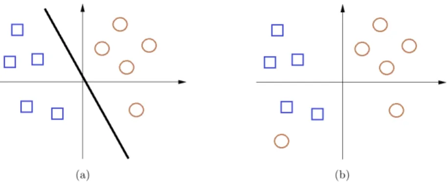
(see Figure 1), such as the exclusive or (XOR1) function.
Figure 1: Linear versus nonlinear separability: (a) Linearly separable function, and (b) non linearly separable function. Circles and squares designate points in two different classes
The key for later advances was the invention of the error
backpropaga-tion learning algorithm by Werbos [36] in combinabackpropaga-tion with multilayer
net-works (explained ahead). Since then, along with the computers evolution to
greater processing power, ANNs have become increasingly popular in many
fields of business, industry and science [38]. There are very recent applications
in health: prognoses in hepatitis C [6] and respiratory abnormalities [2]. In
Sci-ence, ANNs have taken an important role in speech recognition [10], robotics
1XOR represents the inequality function, i.e., the output is 1 if the inputs are not alike,
and vision [14]. ANNs have also been used to predict or classify economic and
financial variables such as the gross domestic product [33], the unemployment
rate [19], inflation [4], exchange rates [22], sovereign risk rating [8], prices of
derivatives [18], futures trading volume [40], credit risk evaluation [1],
mu-tual funds value [5], prediction of financial crashes [29], bank bankruptcy [25],
electricity [26] and water demands [20].
The investigation of Artificial Neural Networks applied to business and
economic forecast is therefore extensive, particularly of stock returns forecast
[39], due to the incentive of achieving substantial monetary rewards. However,
few studies have developed neural networks for individual companies [39].
2.1
Artificial Neural Networks
A neural network is essentially a set of simple processing units (neurons)
that communicate by sending signals through a high number of connections
[14]. Biologically, each neuron receives information from the ”input” neurons,
by ramifications designated as dentrites (see Figure 2). Then the neuron fires
electrical and chemical signals through a channel called axon, if some
thresh-old is reached. Next, the axon is divided into small channels (synapses), and
finally again in dentrites, until the next neurons up in the chain. Human brain
is composed by about 10 billion neurons and it is believed that all knowledge
and experience is encoded by the connections between them.
John von Neumann [21] designed a model that describes a processing unit
for an electronic digital computer. This processor works at a very high speed,
sequentially and is well constrained when compared with a biological neuron.
ANNs attempt to use some principles believed to be used by the human brain,
like adaptivity, fault tolerance and generalization ability (characteristics not
present in von Neumann’s model), combining a large number of processor units
working in parallel in relatively simple tasks and easier to understand.
There are two main groups of ANN models: feedforward and recurrent.
Feedforward refers to the direction of the network’s operation: data flows from
the inputs to the output. In recurrent ones the output of the network is fed back
to the input units using additional feedback connections [27], that allows the
network to exhibit dynamic behaviour over time. Artificial Neural Networks
are a type of machine learning algorithms, a branch of artificial intelligence.
In 1959, Arthur Samuel defined machine learning as a field of study that gives
computers the ability to learn without being explicitly programmed [31]. This
corresponds to the process of refining a model, that learns from experience
(sample or training data), in order to be used in forecasting.
There are three main types of learning algorithms: supervised learning,
unsupervised learning and reinforcement learning. In supervised learning we
want the neural network to act correctly, minimizing a specified error function,
because we know the correct action for every input in our sample. When data is
unlabelled, there is no error or reward signal to evaluate a potential solution.
In such a case, unsupervised learning (e.g. data clustering) tries to find its
hidden structure. In reinforcement learning, the correct input/output pairs are
never presented. Monte Carlo methods are a popular class of reinforcement
learning algorithms. There are also hybrid learning algorithms, which combine
Widrow and Hoff [37] designated artificial neurons by adaptive linear
ele-ments and described the output of one such as:
f(x;w) = G(xTw) (1)
where xis the vector of inputs and w= (w0, ..., wn)T is the vector of weights
assigned to each input xi.
The function Gis known as a transfer (or activation) function and setting
G(xTw) = xTw, we arrive to a simple linear model, standard in
economet-ric modelling. Kuan and White [15] point out that for the logistic function
G(xTw) = 1
1+e−(xTw) , we get the logit model, and when G(x
Tw) is a normal
cumulative distribution function, we obtain a binary probit.
Later, Werbos [36] and Rumelhart, Hinton and Williams [30] combined
such neurons into one function and called them multilayer perceptron, an ANN
composed of at least three layers (see Figure 3).
Figure 3: Structure of a multilayer perceptron
The input neurons xi (i = 1,2, ..., n) represent the explanatory variables
called the hidden layer and is where neurons are attached to transfer functions
and become referred to hidden neurons. Finally, in the last layer there is the
network output. Each input neuron is connected to every neuron in the
hid-den layer by a propagation functionz. The most used is the linear, a weighted combination of the input variables, defined as:
z(x;w) = w0+
n X
i=1
xiwi (2)
A similar function is used connecting the second layer and the output. The
function of a multilayer perceptron can be represented as:
f(x;w;β) =F
H
X
h=0
G(x;w)βh
(3)
whereβ = (β0, ..., βH) is the vector of weights assigned to each hidden neuron.
The output neuron has also a transfer function, represented in equation (3) by
F. In this dissertation I will use the identity function in the final layer, that allows the output to take values in R, which is in our interest since we want
to predict returns. For instance, setting F to be a logistic function may be a relevant way for modelling probabilities.
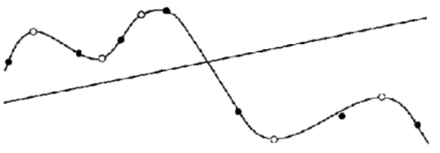
There are other transfer (activation) maps available (see Figure 4), such as
the hyperbolic tangent, a sigmoid function.
The original perceptron of 1957 has a binary transfer function, a type of
step functions that have the significant limitation of not being differentiable.
Radial basis are also a very popular alternative for activation functions (see
appendix B).
Once the network architecture is defined it becomes necessary to estimate
the various weights assigned to each input. Werbos [36] developed an
algo-rithm, the backpropagation, which would come to be the most widely used
[9, 35, 38].
3
Backpropagation Learning Algorithm
Let the training set T = (xp,tp), with p = 1,2, ..., P patterns, where xp = (xp1, ..., xpn)
T
∈Rnis the input vector andtn = (t
n1, ..., tnd)
T
∈Rdis the target
output. The network computes the outputf(xp;w), wherew= (w
1, ..., wn) is
the vector of weights assigned to each input variable. Define the error function
as follows:
E(w;x;β) = 1 2 P X p=1
tp −f(xp;w;β) 2 (4)
Given a specified multilayer perceptron function f, backpropagation is an al-gorithm that consists in changing the weights of f with the objective of mini-mizing the error. For eachp, the equation comes as follows:
E(x;w, β) = 1 2
t−f(x;w;β)
2
The function used ahead in the experiments has additive propagation
func-tions, H logistic functions at the hidden neurons and an identity function at the output (logistic and identity as transfer functions). The equation is of the
form:
f(x;w;β) =β0+
H X
h=1
βh
1
1 +e− w0h+Piwihxi
(6)
Backpropagation is a generalization of the delta rule (gradient descent), a first
order optimization method. Eachβ andwis adjusted in the opposite direction of the error function’s derivative:
△βh =−η
∂E ∂βh
(7)
△wih=−η
∂E ∂wih
(8)
where η is a constant (normally in the range ]0,1[) known aslearning rate. It represents the magnitude of corrections made to the parameters. Its choice
should be made carefully: values near 1 would cause the algorithm to oscillate
a lot producing bigger errors; values near zero slow the convergence to a
solu-tion. Applied to equations (5) and (6), the partial derivatives with respect to
the error function can be written as:
∂E ∂bh
=
t−f(x;w;β)
∂f ∂bh (9) ∂E ∂wih = H X h=1
t−f(x;w;β)
with G as the logistic function (recallz from equation (2)). There are several variants from the original backpropagation, following the same logic as the
steps below:
1. Start with all weights set to random values between -1 and 1.
2. Submit the first training pattern and obtain the output.
3. Compare the network output with the target output.
4. Correct the output weights using the following formula:
bh =bh+ηδoGh+ (bh×momentum) (11)
where bh is the weight connecting the hidden unit h with the output. η is the
learning rate, Gh is the output at hidden unit h,momentum is a constant and
δo is given by the following:
δo =t−f(x;w;β) (12)
where f is the network output andt is the target.
5. Correct the input weights using the following formula:
wih=wih+ηδhxi+ (wih×momentum) (13)
where wih is the weight connecting the inputxi to the hidden neuron h, xi is
the correspondent input value at the first layer and δh is given by:
δh =Gh(1−Gh) X
h
δowho (14)
6. Calculate de squared error:
E = 1 2
t−f(x;w;β)
2
(15)
7. Repeat from 2 for each pattern in the training set to complete one epoch
or training time.
8. Shuffle the training set randomly (prevents the network being influencend
by the order of the data2).
9. Repeat from step 2 for predefined periods (or until the error ceases to
change, given a predefined threshold).
Note that β0 and w0 are weights assigned to extra inputs which always equal
one, known as bias (recall Figure 3). After multiplying this by the
corre-spondent weight we get the constant term, analogous to the intercept term
in a linear regression. The momentum parameter (typically between 0 and 1)
quantifies the inertia of the weights, forcing them to change direction contrary
to the one which reduces the error. Small values formomentum can accelerate
the convergence. In the equation (14), the sum presented is up to the number
of units that form the hidden layer. Some authors recommend that the sum
(i.e. the number of hidden neurons) should be up to √inputs×outputs [3]. Others argue that the optimal number will generally be found from one-half
to three times the number of hidden neurons [13]. Regarding the number of
hidden layers, multilayer perceptron models with just one hidden layer, since
a sufficient number of hidden neurons is provided, are universal approximators
[12] and the most effectively used.
2Is the most recent data available more important or is it just the relatioship betwen the
3.1
Advantages and Disadvantages
The main advantage of artificial neural networks is that they belong to the
class of nonparametric models, so there is no requirement about the
distri-bution of the data, the availability of multiple training algorithms and their
nonlinear configuration. Empirical observations suggest that when complex
nonlinear relationships exist in data sets, neural networks models may provide
a tighter model fit than conventional regression techniques. They can
accu-rately capture complex patterns in existing information, allow for categorical
data and have no restrictive assumptions. Neural networks also perform well
with missing or incomplete data.
On the other hand, there are no structured criteria for the choice of the
parameters, like the number of hidden layers or hidden neurons, the learning
rate or the training time, etc. Such flexibility involves much trial and error
until the right combination of the parameters is reached. Furthermore, there
are no economic reasons to justify which combination is more appropriated. It
is also difficult to understand how the relationship between hidden neurons are
estimated as well as to interpret in economic or financial terms each weight
separately. This limitation is referred to as the black box criticism. There
is also tendency to overfitting (see Figure 5) due to the large number of free
parameters.
There can be also complexity costs when more than one hidden layer is
used or large training periods: neural networks can be time consuming.
At last, algorithms for artificial neural networks were conceived to converge
to a local minimum of the error function, not the global. However, global
optimization is a big challenge in what concerns computation. Note that
nor-malizing the data, although not required, can improve the performance of the
networks.
4
Traditional Regression Models
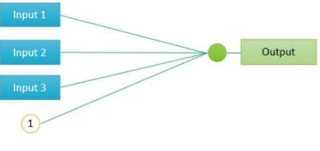
Neural networks are similar to linear and nonlinear least squares regression.
Autoregressive and multiple linear regression models may be seen as
feedfor-ward neural networks with no hidden layers, i.e. single layer networks3 (see
figure 6) and one output neuron equipped with a linear transfer function.
Figure 6: Example of a Single layer network
A Logistic regression model (with no interaction terms) is also identical to
a single layer network (but, with logistic function as transfer function).
How-ever, in logistic regressions, the process converges when the likelihood function
is maximized whereas in a neural network it is usually a least squares error
3Some authors don’t consider the input variables forming a layer, because of their
function that is minimized (although likelihood functions can be maximized
too). Spackman [32] has shown that a single layer backpropagation neural
net-work developed using a maximum likelihood objective function will converge
to the same solution as a plain logistic regression model. In Table 1 there is a
brief glossary showing some popular terms in the field of neural networks and
their equivalents in statistics. A big separation between traditional statistical
methods and ANNs resides in post estimation analysis. The former have tests
of significance for input variables and confidence intervals for output variables.
Comparable tests are not generally available for the latter. Empirical studies
drew attention to the fact that financial time series exhibit nonlinear effects,
and often fail to verify traditional assumptions of econometrics, such as the
normality, stationary, independence and homoscedasticity of the residuals. In
this work, I explore neural networks as an alternative against traditional linear
regressions (architectures presented in section 5.4).
Neural Networks aaaaaaaaaaaaaaaaStatistics
Input, attribute aaaaaaaaaaaaaaaaIndependent variable Output aaaaaaaaaaaaaaaaDependent Variable Connection weights aaaaaaaaaaaaaaaaRegression coefficients Bias weight aaaaaaaaaaaaaaaaIntercept Parameter Error aaaaaaaaaaaaaaaaResiduals
Learning, training aaaaaaaaaaaaaaaaParameter estimation Training case, instance aaaaaaaaaaaaaaaaObservation
Cross-entropy aaaaaaaaaaaaaaaaMaximum likelihood estimation
Table 1: Common terms in the field of neural networks and statistics.
5
Oil & Gas Industry
Half of the twenty biggest companies in 2012, by revenue, are from the oil and
the functioning of the industrialized civilization itself. It is used for a vast and
ever growing-range of purposes: oil to fuel automobiles and airplanes, plastics,
natural gas for heating and increasingly as fuel, etc.
The Chicago Mercantile Exchange Group and the New York Mercantile
Exchange (NYMEX) are the exchange companies where the most liquid
con-tracts of crude oil and natural gas futures are negotiated, respectively. The
price of crude oil futures is often referenced in news reports, historically
mov-ing close to the price of Brent crude searched and explored in the North Sea,
that is the leading global price benchmark for crude oil. Although most Brent
is destined for European markets, it has been used as benchmark by all West
African, Mediterranean and some Southeast Asia crudes.
Energy companies, such as Exxon Mobil, Royal Dutch Shell, BP, Total,
Repsol and Galp Energia operate worldwide in this field as integrated
com-panies: after extracting oil and gas to the surface (upstream sector), they
transport the raw materials principally through pipelines to refineries and,
in the end, deliver the various refined products to downstream distributors.
These companies were chosen for our experiments with ANNs.
5.1
Networks Architecture
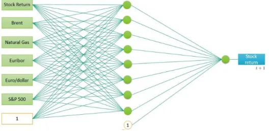
All the neural network models estimated have six input variables that can
be good predictors of the next day’s share price of each company.
Lett+ 1 be the day for which the prediction is made. The input variables are the returns observed in the market in daytof: company’s share price, Brent crude futures contract price, natural gas futures contract price, 3 month euribor
rate, euro to U.S. dollar exchange rate and Standard & Poor’s 500 index. Let
the price of the asset be defined by the time series {Pt} , t = 0,1,2, .... The
returnRt in someday t is defined as: Rt=
Pt−Pt−1
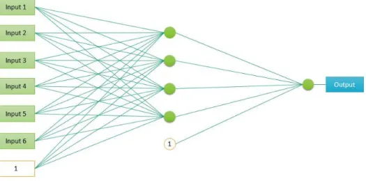
Figure 7: Multilayer perceptron with four hidden units
For each company, a neural network with 4 hidden neurons (see Figure 7)
and another model with 8 hidden units (see Figure 8) were implemented. Both
were trained with 1567 observations, taken from Datastream, corresponding
to the period from 01-Jan-2007 to 31-Dec-2012. Thelearning rate was 0.3 and
the momentum 0.1. The networks were trained for 100 epochs. The software used was WEKA (Waikato Environment for Knowledge Analysis), an open
source based on JAVA, popular in the machine learning community.
5.2
Investor Strategy
The strategy of the hypothetical investor is at first step, on a daily basis: in
31/Dec/2012 following the close of the NASDAQ stock market, the network
makes a prediction for the return of each stock for the first trading day of 2013.
If the return predicted by the network is greater than zero, then the investor
takes a long position, hoping for an appreciation of the share price. If the return
predicted by the network is less than zero, the investor takes a short position,
betting on a price decline. If the forecast is correct, the profit, corresponding
to the effective price movement: Pt−Pt−1
Pt is collected. If the opposite occurs,
a loss is incurred. When the U.S. market closes in 02-Jan, a new model is
estimated including the latest information and a new prediction is performed,
but now, for the next negotiations day, 03-Jan. If the network predicts the
same direction for the share movement as the day earlier, then the investor
holds his position, otherwise he closes the position and bets in the opposite
way. We assume that the markets are highly liquid. This assures that when
the market opens our order is immediately matched, so that makes the daily
change in prices to correspond precisely to the variation (in the same direction
or not) of the investor returns. For simplicity, we also suppose that there are
no transaction costs. Institutional investors, like banks, insurance companies
or hedge funds have some ease mitigating them, through the movement of large
sums of cash. For a particular investor, it may be desirable to take them into
account.
5.3
Economic Relevance
It is easy to verify, with the accounts report, the exposure to risk big
interest rate risk and the exchange rate risk.
The market risk, also known as systematic risk, cannot be eliminated
through portfolio diversification (but it can be hedged against). For instance,
a recession or political turmoil environment cause a decline in the market as
a whole. As a result, the stocks will fall, depending on the correlated
volatil-ity of the stocks in relation to the market movements. A popular measure of
market risk is the beta (β), from the Capital Asset Pricing Model (CAPM). The higher the beta4, the higher is the market risk associated to that stock.
A large part of coupons paid by companies, as underwriters of bonds,
con-sist in a float reference interest rate plus a spread on a given nominal amount.
In the case of interest rate risk, if our proxy for the float rate, the euribor
(normally at 3 and 6 months maturities) goes up then difficulties rise for
com-panies paying their interests on borrowings. It is also expected a deviation
from investments in stocks to investments in bonds, offering higher yields. On
the other hand, low rates make the fixed income market less attractive. The
Euro Interbank Offered Rate (Euribor) is based on the interest rates at which
a panel of big European banks borrow funds between them. In the
calcula-tion, published every day by the European Banking Federacalcula-tion, the highest
and lowest 15 of all the quotes collected are eliminated. The remaining rates
are averaged. Euribor provides the basis for the price or interest rate of all
kinds of financial products, like corporate bonds.
In the case of Exxon Mobil, for an interest rate risk proxy we used the
LIBOR (London Interbank Offered Rate). The LIBOR is the world’s most
widely used benchmark for short-term interest rates. It is calculated by British
Bankers’ Association in a similar way to the euribor, but on a global scale. In
4Beta is obtained using historical data and computing the covariance between the rates
the United States, many adjustable rates in fixed income market are indexed
to the LIBOR.
Multinational firms are participants in currency markets due to their
inter-national operations. Therefore, this type of companies are subject to exchange
rate risk, due to changes in currency exchange rates, which can adversely affect
profit margins. The exchange rate between the euro and the U.S. dollar is the
most negotiated in the world and it is relatively stable. The U.S. dollar is the
most liquid currency in the forex market. Nearly every central bank and
in-stitutional investors in the world holds this currency, and some countries (e.g.
many countries in Central America) use it as an official or unofficial alternative
to their local currencies or as an exchange-rate peg. In our experiments we use
the exchange rate from euro to U.S. dollar as a proxy for exchange rate risk
and the U.S dollar to the British pound sterling in the case of BP.
The enterprises on this kind of industry are naturally exposed to
fluctu-ating prices of crude oil, natural gas, oil products and chemicals. Factors
that influence supply and demand include natural disasters, weather, political
instability, conflicts, economic conditions and actions by major oil-exporting
countries. For instance, in a low oil and gas price environment, the company
would generate less revenue from its upstream production and, as a result,
cer-tain long-term projects might become less profitable, or even incur in losses.
In the future, the prices of these commodities can be unaffordable given the
increasing demand by emerging economies combined with the need of measures
to reduce CO2 emissions.
Other risk factors, such as the probability of credit events or changes in
securities tax lax, although also important, are not considered in our models
5.4
Conventional Models Architecture
In our experiments we tested the neural networks presented in subsection 5.1
against the linear models presented next. Letytbe the return for the company
in study in the moment t. The following model describes the returns of this company as a linear combination of predictor variables:
yt =b0+b1yt−1+b2brentt−1+b3gast−1+b4excht−1+b5indext−1+b6euribt−1+ut
(16)
wherebrent is the return of the Brent crude oil future contracts prices; gasis the return of the natural gas futures contact prices; exch is the variation on the Euro to U.S. dollar; the eurib is the change in the 3 month euribor rate;
indexcorresponds to the S&P 500 index return and utbeing independent and
identically distributed (iid) random variables . This model falls into the class of autoregressive moving average models with exogenous inputs (ARMAX).
Autoregressive AR(1) models are also used:
yt =c+φ1yt−1+ut (17)
with|φ1|<1 and ut being iid random variables. This model belongs the class
of stationary5 linear processes (moving average models also belong to this
category) and is an important model in Finance, given that it can reasonably
reproduce the dynamics of many time series. Random walks, autoregressive
but nonstationary (evolutive) processes, are also used in our tests:
yt=c+yt−1+ut (18)
with ut being a white noise independent from yt−1.
6
Results
For models results evaluation we used the network’s final return, the root
mean squared error (RMSE6), the mean absolute error (MAE7), and the
per-centage of correct predictions on price movements direction and the sharp
ratio. The results are shown in Tables 2-7. In the application of ANNs with
eight hidden units, Galp Energia gave 16.9% of profitability, Repsol 22.92%
and Total 27.27%, in the period of four months. In our experiments, neural
networks didn’t perform so well predicting the direction of stocks prices from
BP, which gave us 5.62% of returns, Shell (-0.55%) and Exxon (5.18%). It is
in the separation between the companies whose ANNs performance were good
and those were results were poorer, that we will derive our conclusions. The
real stocks returns observed for each company in the market during the study
period appear in the tables in the ”Benchmark” row.
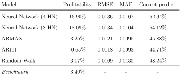
Model Profitability RMSE MAE Correct predict.
Neural Network (4 HN) 16.90% 0.0136 0.0107 52.94%
Neural Network (8 HN) 18.09% 0.0134 0.0104 54.12%
ARMAX 3.25% 0.0121 0.0095 45.88%
AR(1) -0.65% 0.0118 0.0093 44.71%
Random Walk 3.17% 0.0169 0.0135 48.24%
Benchmark 3.49% - -
-Table 2: Galp Energia results
a
6RM SE=q2 PNi=1(ti−oi)2
N
7M AE = 1
N
PN
i=1|ti−oi|= N1 P N
i=1|ei|. In the experimentsN equals 85, the number
of negotiations days under study. ti corresponds to the target/real observed return at day
Model Profitability RMSE MAE Correct predict.
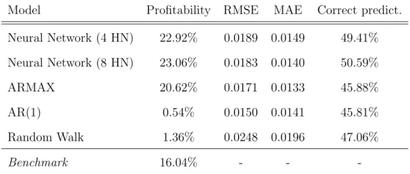
Neural Network (4 HN) 22.92% 0.0189 0.0149 49.41%
Neural Network (8 HN) 23.06% 0.0183 0.0140 50.59%
ARMAX 20.62% 0.0171 0.0133 45.88%
AR(1) 0.54% 0.0150 0.0141 45.81%
Random Walk 1.36% 0.0248 0.0196 47.06%
Benchmark 16.04% - -
-Table 3: Repsol results
Model Profitability RMSE MAE Correct predict.
Neural Network (4 HN) 27.27% 0.0140 0.0109 51.76%
Neural Network (8 HN) 29.08% 0.0132 0.0107 52.94%
ARMAX 11.57% 0.0122 0.0094 50.59%
AR(1) -5.54% 0.0123 0.0094 41.18%
Random Walk 4.66% 0.0211 0.0164 55.29%
Benchmark -1.90% - -
-Table 4: Total results
Model Profitability RMSE MAE Correct predict.
Neural Network (4 HN) 5.62% 0.0117 0.0095 52.94%
Neural Network (8 HN) 7.76% 0.0117 0.0095 50.59%
ARMAX 0.81% 0.010 0.0076 45.88%
AR(1) -9.49% 0.0111 0.0078 49.41%
Random Walk 8.77% 0.0188 0.0145 51.76%
Benchmark 9.79% - -
Model Profitability RMSE MAE Correct predict.
Neural Network (4 HN) -0.55% 0.0105 0.0078 51.76%
Neural Network (8 HN) 1.41% 0.0107 0.0081 52.94%
ARMAX 0.04% 0.009 0.0057 47.06%
AR(1) -12.05% 0.0077 0.0057 34.12%
Random Walk 3.96% 0.0176 0.0136 47.06%
Benchmark -0.58% - -
-Table 6: Royal Dutch Shell results
Model Profitability RMSE MAE Correct predict.
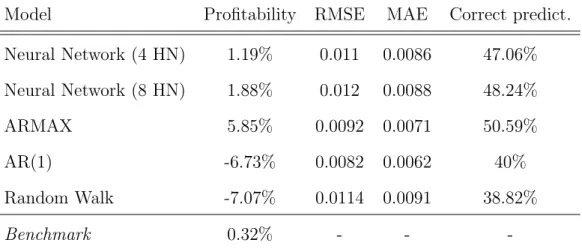
Neural Network (4 HN) 1.19% 0.011 0.0086 47.06%
Neural Network (8 HN) 1.88% 0.012 0.0088 48.24%
ARMAX 5.85% 0.0092 0.0071 50.59%
AR(1) -6.73% 0.0082 0.0062 40%
Random Walk -7.07% 0.0114 0.0091 38.82%
Benchmark 0.32% - -
-Table 7: Exxon Mobil results
6.1
Results evaluation
ANNs with 8 hidden units were the best models in what concerns the final
return. Autoregressive models always provided better results in terms of root
mean square error and mean absolute error (see appendix C). Most models
had a direction accuracy around fifty percent. Benchmarks were largely beat
in Galp, Repsol and Total experiment’s concerning ANNs. In some cases,
random walks performed results in terms of correct predictions close to the
6.1.1 Number of Synapse Connections
Artificial neural networks with 8 hidden neurons presented better results
than ANNs with the same learning rate, training time and momentum but
with 4 hidden neurons. The former seem to detect non linearities that the
latter ones do not. We can think of simply add hidden units to our network
hopping even better results. However, parameters estimation can be much
more time consuming adding hidden neurons as well as increasing the number
of hidden layers, input variables or training time. Let ni be the number of
neurons (bias excluded) in layer i (n1 equals the number of input variables)
from an ANN with L layers. The number of parameters to be estimated is described by the following formula:
L−1
X
i=1
(ni + 1)ni+1 = (n1+ 1)n2+ (n2+ 1)n3+...+ (nL−2+ 1)nL−1 (19)
In the experiments, with 6-4-1 and 6-8-1 architectures, for ANNs with four
hidden units there were estimated 33 parameters, whereas in ANNs with 8
hidden units there were estimated 64. Lack of parsimony is evident when
compared with the AR(1) and ARMAX models. In tests, just 2 and 7
param-eters were estimated per model, respectively.
6.1.2 Companies Market Cap
In a deeper analysis, the need of testing directional forecast values arises
because, although biased forecasts occur, investors still profit if they are on
the correct side of the price change more often than not. Pesaran and
Timmer-mann [23] built a statistic to test if stocks prices directions are independent
from directions given by models. This is the null hypothesis, which suggests
ex-plained bellow. LetP denote the correct direction predictions of the network:
P = N1 PNt=1Dt a, a whered Dt =
1, if TtYt>0
0, otherwise
P = 1 means perfect direction accuracy, whereas P = 0 means that any correct prediction is made.
Leta At=
1, if Tt>0
0, otherwise
; aBt=
1, if Yt>0
0, otherwise ;
PA= N1 PN
t=1At a;a PB = N1 PN
t=1Bt a and aP∗ =PAPB+ (1−PA)(1−PB).
Pesaran and Timmermann’s statistic, defined as: P T = P−P∗
[V(P)−V(P∗)]
1 2
a
∼N(0,1) follows a standardized asymptotic normal distribution with hypothesis:
•H0: Tt and Yt independent random variables.
•H1: H0 false.
V(P) and V(P∗) represent the variances from P and P∗ respectively, defined by the following:
V(P) =N−1P
∗(1−P∗) a;
V(P∗) = N−1(2P
B−1)2PA(1−PA)+N−1(2PA−1)2PB(1−PB)+4N−2PBPA(1−
PB)(1−PA)
Using this statistic for each company in the period of study, the null hypothesis
Not even the ANNs for Galp, Repsol and Total, which provided good final
results? Filtering all observed returns into big returns (we considered the ones
with an absolute return greater than 1%) and small returns (otherwise) and
gathering the big returns of Galp, Repsol and Total for a joint evaluation on
the single Pesaran and Timmermann’s statistic, we get a p-value of 0.0427.
Contrary, the null hypothesis is clearly not rejected again when testing for the
big returns of BP, Shell and Exxon together. This statistic was made in the
circumstances presented above by the following reasons. First: the number
of big returns is lower than the number of total returns: increasing the
num-ber of observations by grouping observations in a statistic improves results’
reliability. Second: groupings were made concerning companies’ market
capi-talization8, i.e. the stock price multiplied by the number of shares outstanding,
by separating the three companies with lower market cap from the three ones
with biggest. The main reason of the separation by indicator is that ANNs
performed better for those with lower market cap (see Figure 9).
Figure 9: ANN with 8 hidden neurons return & company market capitalization (return in %, market cap in 1010 US dollars)
We believe ANNs capture better investors overall expectations for next
negotiation’s day given what happened in the previous day in the market for
the companies with lower market cap, according to the “small firm effect”,
which argues that those tend to have a volatile business environment, more
vulnerable to what happens in the markets, beyond having lower stock prices,
which means that price appreciations tend to be larger than socks with a bigger
market capitalization. Fama and French [7] used this separation (small minus
big) as a relevant input in the three factor model for equity portfolios.
In Table 8 there are the beta coefficients resultants by estimating the
re-gression of each company’s returns against the Standard & Poor’s 500 index
under the tests period.
Company Galp Repsol Total BP Shell Exxon
beta 0.78 1.31 0.97 0.41 0.46 0.69
T-Stat9 9.05* 5.79* 6.03* 2.76** 4.21* 3.99*
Table 8: Companies against market regressions
There were obtained higher betas for the three companies with lower market
capitalization: Galp, Repsol and Total. This supports the thesis of more
vulnerability for lower cap firms. It’s important to take into account that
Exxon Mobil is the major component of the North America Market’s Index
(S&P 500) and even then gave us lower correlation with his home market than
the ”foreign” lower cap companies, in some way revealing the idiosyncratic
effects that the behaviour of financial markets in North America places in
Europe. This type of risk has received some attention by the development of
multivariate models and hypothesis tests, such as the Granger causality, to
test co-movements of return and volatility between financial time series.
6.1.3 Sharpe Ratio
The Sharpe Ratio, defined as:
S = Rp−Rf
σp
(20)
wereRp is the average or expected value of the returns on the portfolio,Rf the
risk-free10 rate and σ
p is the portfolio standard deviation, indicates how well
the return of an asset rewards the investor for the risk taken. It is a simple
way to evaluate the performance of a portfolio. When comparing two assets
versus a common benchmark (risk free rate in our experiments), the one with
a higher Sharpe ratio provides a better return for the same risk.
Figure 10: Sharpe Ratio results
Artificial Neural Networks with eight hidden neurons were the bests
mod-els in what concerns the trade-off between risk and return, concerning Galp,
Repsol and Total trading performance. For the three biggest companies in
terms of market cap one cannot draw any relevant conclusions.
10The risk-free rate to 4 months was determined by linear interpolation between the
7
Conclusion
This work applies artificial neural network (ANN) models against
autore-gressive and multiple linear models in order to investigate their performance
detecting asset price movements quoted in stock exchanges. It were used the
daily returns of future contracts on Brent crude and natural gas, the returns
of the exchange rate between the currencies euro and U.S. dollar and the stock
returns of Galp, Repsol, Total, BP, Shell and Exxon Mobil (1651 observations)
in our models as inputs to predict stocks prices movements for these companies
for the following day, for a period of four months. Two multilayer perceptrons,
with 6-4-1 and 6-8-1 architectures and logistic activation functions in the
hid-den layer and ihid-dentity at the output learned with those patterns.
Neural Networks were the best models in the experiments, in terms of final
return. It was found that multilayer perceptrons with eight hidden units in
the hidden layer predicted better the returns than multilayer perceptrons with
four hidden units, ceteris paribus.
The ANNs predicting big return’s direction (we considered the ones in
module greater than 1%) provided good results for companies under study
with lower market capitalization. One may conjecture that ANNs capture
better overall investors expectations for next negotiation’s day, given what
happened in the previous day in the markets for the companies with lower
market cap, according to the “small firm effect”, which argues that those tend
to have a volatile business environment, more vulnerable to what happens
in the markets, despite having lower stock prices, which means that price
appreciations tend to be larger than socks with a bigger market capitalization.
Fama and French used this separation (small minus big) as a relevant input in
models always provided better results in terms of root mean squared error and
mean squared error.
Results suggest multilayer perceptron models may serve as a good
alterna-tive tool to traditional econometric regressions for forecasting financial
mar-kets, specially for institutional investors. In fact, these are big sponsors of
this type of research. However, models accuracy is difficult to obtain and can
take months of investigation. Neural network software that allow automated
routines or direct programming skills are desirable.
Given that in our experiments linear models provided better results in
terms of RMSE and MAE, we suggest the combination in a synergistic way
of both traditional regression models and artificial neural networks for time
series forecasting.
There are many other possible extensions to this work. For the followers
of technical analysis, technical indicators such as the Relative Strength Index
(RSI), Bollinger Bands or Moving Average could be good predictor variables
for price movements. Bloomberg believes that in 2020 Singapore will be the
largest wealth manager in the world. A possible extension to enhance profits
is through the application of neural networks in financial markets with strong
growth potential (e.g. Singapore).
For other areas of Finance, such as risk management, given the
empiri-cal evidence that volatilities of financial time series exhibit lower decays is
their autocorrelation functions when compared to the returns, we recommend
the application of neural networks to predict this risk measure for portfolio
managers in contrast to the popular ARCH and GARCH models.
For static modelling, we consider the application of neural networks to fit
term structures as opposed to the most used indirect methods, like the
References
[1] Angelini, E., Tollo, G. & Roli, A. (2008). A neural network approach for credit risk evaluation. The Quarterly Review of Economics and Finance
48, 733–755.
[2] Baemani, M. J., Monadjemi, A. & Moallem, P. (2008). Detection of Res-piratory Abnormalities Using Artificial Neural Networks.Journal of Com-puter Science 4(8), 663-667.
[3] Kaastra, I., & Boyd, M. (1996). Designing a neural network for forecasting financial and economic time series. Neurocomputing 10(3), 215-236.
[4] Choudhary, M. A., Haider, A. (2012). Neural Networks for inflation fore-casting: an appraisal. Applied Economics 44, 2631-2635.
[5] Chiang, W. C., Urban, T. L. & Baldridge, G. W. (1996). A neural network approach to mutual fund net asset value forecasting.Omega24(2), 205–215.
[6] Dr˘agulescu, A., Albu, A., Gavrilut˘a, C., Filip, S. & Menyhardt, K. (2006). Statistical Analysis and Artificial Neural Networks for prognoses in Hep-atitis C. Acta Polytechnica Hungarica 3(3), 71-79.
[7] Fama, E. F. & French, K. R. (1992). The Cross-Section of Expected Stock Returns. The Journal of Finance 47(2), 427-466.
[8] Fioramanti, M.(2008). Predicting sovereign debt crises using artificial neu-ral networks: A comparative approach.Journal of Financial Stability 4(2), 149–164.
[9] Fu, L. M. (1994). Neural Networks in Computer Intelligence. New York: McGraw-Hill
[10] Gevaert, W., Tsenov, G. & Mladenov, V. (2010). Neural Networks used for Speech Recognition. Journal of Automatic Control 20, 1-7.
[11] Hinton, G. & Sejnowski (1999). Unsupervised Learning: Foundations of Neural Computation. Unsupervised Learning: Foundation Computation. Cambridge, MA: The MIT Press.
[12] Hornik, K., Stinchcombe, M. & White, H. (1989). Neural Networks 2(5), 359-366.
[13] Katz, J. O. (1992). Developing neural network forecasters for trading.
Technical Analysis of Stocks and Commodities 10(4), 160-168.
[14] Kr¨ose, B. & Smagt, P. V. (1996).An introduction to Neural Networks, 8th
[15] Kuan, C. M. & White H. (1994). Artificial Neural Networks: An Econo-metric Perspective. Econometric Reviews 13, 1-92.
[16] McCulloch, W. & Pitts, W. (1943). A Logical Calculus of Ideas Immanent in Nervous Activity. The Bulletin of Mathematical Biophysics 5, 115-133.
[17] Minsky, M. L. & Papert, S. (1969).Perceptrons: An Introduction to Com-putational Geometry. Cambridge, Massachusetts, USA: The MIT Press.
[18] Morelli, M., Montagna, G., Nicrosini, O., Treccani, M., Farina, M. & Am-ato, P. (2004). Pricing financial derivatives with neural networks. Physica A: Statistical Mechanics and its Applications 338(1–2), 160–165.
[19] Moshiri, S. & Brown, L. (2004). Unemployment Variation over the Busi-ness Cycles: a Comparison of Forecasting Models. Journal of Forecasting
23, 497-511.
[20] Msiza, I. S., Nelwamondo, F. V. & Marwala, T. (2008).Water Demand Prediction using Artificial Neural Networks and Support Vector Regression.
Journal of Computers 3(11), 1-8.
[21] Neumann, J. V. & Alexander, S. N. (1945). First Draft of a Report on the EDVAC. Moore School of Electrical Engineering, University of Penn-sylvania.
[22] Pacelli, V., Bevilacqua., V. & Azzollini, M. (2011). An Artificial Neural Network Model to Forecast Exchange Rates.Journal of Intelligent Learning Systems and Applications 3, 57-69.
[23] Pesaran, M. H. & Timmermann, A. (1992). A Simple Nonparametric Test of Predictive Performance.Journal of Business & Economic Statistics
10(4), 461-465.
[24] Reed, R. & Marks, R. (1999). Neural Smiting: Supervised Learning in Feedforward Artificial Neural Networks. Cambridge, MA: The MIT Press.
[25] Ravi, V. & Pramodh, C. (2008). Threshold accepting trained principal component neural network and feature subset selection: Application to bankruptcy prediction in banks. Applied Soft Computing 8, 1539–1548.
[26] Ringwood, J. V., Bofelli, D., & Murray, F. T. (2001). Forecasting Elec-tricity Demand on Short, Medium and Long Time Scales Using Neural Networks. Journal of Intelligent and Robotic Systems 31, 129-147.
[28] Rosenblatt, F. (1958). The perceptron: A probabilistic model for infor-mation storage and organization in the brain. Psychological Review 65(6), 386-408.
[29] Rotundo, G. (2004). The perceptron: Neural networks for large finan-cial crashes forecast. Physica A: Statistical Mechanics and its Applications
344(1–2), 77–80.
[30] Rumelhart, D. E., Hinton, G. E. & Williams, R. J. (1986). Learning in-ternal representations by error propagation. Parallel distributed processing
1, 318-363.
[31] Simon, P.(2013). Too Big to Ignore: The Business Case for Big Data. New Jersey: Wiley.
[32] Spackman, K. A. (1992). Combining logistic regression and neural net-works to create predictive models. Proceedings of the Sixteenth Annual Symposium on Computer Applications in Medical Care 456-459.
[33] Tkacz, G. (2001). Neural network forecasting of Canadian GDP growth.
International Journal of Forecasting 17, 57-69.
[34] Tu, J. V. (1996). Advantages and disadvantages of using artificial neural networks versus logistic regression for predicting medical outcomes.Journal of Clinical Epidemiology 49(11), 1225–1231.
[35] Walczak, S. & Cerpa, N. (1999). Heuristic Principles for the design of artificial neural networks.Information And Software Technology 41(2), 109-119.
[36] Werbos, P. J. (1974). Beyond Regression: News Tools for Prediction and Analysis in the Behavioural Sciences. Harvard University, PhD thesis.
[37] Widrow, B. & Hoff, M. E. (1969) Adaptive Switching Circuits. IRE WESCON Convention Record 4, 96-104.
[38] Widrow, B., Rumelhart, D. E., & Lehr, M. A. (1994). Neural Networks: Applications in industry, business and science. Communications of the ACM 37(3), 93-105.
[39] Zhang, P. (2004).Neural Networks in Business Forecasting. Hershey, PA: Idea Group Publishing.
Appendix A
ADALINE
Adaptive linear neuron (ADALINE) is a function with n input neurons xi,
each one assigned with one weight wi. The output y can be defined by the
following equation:
y=
n X
i=1
wixi (21)
After an initial assignment of random values (typically small ones) to the
weights, the fitting is made by adjusting the weights with the following rule:
wnew=wold+η(ˆy−y)x (22)
withηconstant, ˆythe value given by the model andybeing the target. This process is repeated until a minimum specified value of the error functionE = (ˆy−y)2 is achieved. This value and the η are defined by the mathematician,
according to the results recorded.
Appendix B
Radial Basis Networks
Radial Basis Networks (RBNs) are a popular class of multilayer feed-forward
networks that employs radial basis functions as the activation ones. A RBN,
s, is a scalar function of the input vector, φ :Rn→
R, and is of the form:
s(x) =
N X
i=1
λiφ x−ci
(23)
where ci is the center vector for neuron i, and λi is the weight of neuron i in
The mapφis called basic function. Every function can be represented as a linear combination of basis functions. For instance, a quadratic polynomial of
the formx2+bx+chas {x2, x,1} as basis. Popular choices of basic functions
include (writing r= x−ci
):
• gaussian kernel: φ(r) =e−(ǫr)2
• multiquadratic: φ(r) =√r2+c2 , c >0
• thin plate spline : φ(r) = r2ln(r)
Jointly, the hidden units provide a set of functions that constitute a flexible
basis set for representing input patterns (see Figure 10).
Appendix C
Error Performance Plots
Figure 12: Galp error plots from ANN (8 HN) in blue and AR(1) in red
Figure 13: Repsol error plots from ANN (8 HN) in blue and AR(1) in red
Figure 15: BP error plots from ANN (8 HN) in blue and AR(1) in red
Figure 16: Shell error plots from ANN (8 HN) in blue and AR(1) in red
![Figure 2: A biological neuron representation [24]](https://thumb-eu.123doks.com/thumbv2/123dok_br/16895988.756944/13.892.299.599.955.1052/figure-a-biological-neuron-representation.webp)
![Figure 4: Transfer functions [11]](https://thumb-eu.123doks.com/thumbv2/123dok_br/16895988.756944/16.892.220.670.896.1034/figure-transfer-functions.webp)