Modeling and numerical simulation of slurry flow / Modelagem e simulação numérica de escoamento de polpa

(1)

Braz. J. of Develop., Curitiba, v. 5, n. 10, p. 20462-20477, out. 2019. ISSN 2525-8761

Modeling and numerical simulation of slurry flow

Modelagem e simulação numérica de escoamento de polpa

DOI:10.34117/bjdv5n10-233

Recebimento dos originais: 20/09/2019 Aceitação para publicação: 18/10/2019

João Rodolfo Januário

Mestre em Engenharia Mecânica pela Pontifícia Universidade Católica de Minas Gerais Instituição: Pontifícia Universidade Católica de Minas Gerais

Endereço: Av. Dom José Gaspar, 500 – Coração Eucarístico, Belo Horizonte – MG, Brasil E-mail: joaorjanuario@gmail.com

Cristiana Brasil Maia

Doutora em Engenharia Mecânica pela Universidade Federal de Minas Gerais Instituição: Pontifícia Universidade Católica de Minas Gerais

Endereço: Av. Dom José Gaspar, 500 – Coração Eucarístico, Belo Horizonte – MG, Brasil E-mail: joaorjanuario@gmail.com

ABSTRACT

The objective of the present study was to implement distinct non-Newtonian fluid theories of heterogeneous mixture between water and minerals, aiming to identify the advantages and limitations of each model. Different CFD methodologies were associated with characterization methods of fluids and validated using experimental literature data to be used as a tool to calculate pressure losses in a pipe. With the results obtained, the most efficient methodology to simulate this type of flow can be chosen. The methods contemplated the use of equivalent viscosity and variable viscosity. Equivalent viscosity results were closer than the variable viscosity results to experimental data, however, the variable viscosity model did not require experimental data to interpolate the boundary conditions.

Keywords: Mineral pulps; Critical velocity; Slurry flow; Non-Newtonian fluids; equivalent

viscosity; variable viscosity.

RESUMO

O objetivo do presente estudo foi implementar diferentes teorias não-newtonianas de fluidos de mistura heterogênea entre água e minerais, com o objetivo de identificar as vantagens e limitações de cada modelo. Diferentes metodologias de CFD foram associadas aos métodos de caracterização de fluidos e validadas utilizando dados da literatura experimental para serem utilizados como uma ferramenta para calcular as perdas de pressão em um tubo. Com os resultados obtidos, pode-se escolher a metodologia mais eficiente para simular esse tipo de fluxo. Os métodos contemplaram o uso de viscosidade equivalente e viscosidade variável. Resultados de viscosidade equivalentes foram mais próximos do que os resultados de viscosidade variável aos dados experimentais; no entanto, o modelo de viscosidade variável não exigiu dados experimentais para interpolar as condições de contorno.

(2)

Palavras-chave: Polpas minerais; Velocidade crítica; Fluxo de chorume; Fluidos não newtonianos; viscosidade equivalente; viscosidade variável.

1. INTRODUCTION

Transportation of solids through pipelines are widely used in many industrial applications (Singh et al, 2017). A broad variety of processes produce slurry flows of different properties and behaviors. Due to this extensive production, the determination of the pipeline transport characteristics is a very useful tool for improving the efficiency and safety of the structure.

The slurry is usually considered as a non-Newtonian fluid. Depending on the characteristics of the slurry, different models can be used to characterize it. It can be defined as Bingham fluid to simplify calculation for engineering purposes (Frigaard et al, 2017), but, in general, the fluid characteristics are more complex and demand more refined models. Most common models are Power law, Bingham and Herschel-Bulkley models (Min et al, 2018). The literature presents several papers using experimental, analytical and numerical models to study the slurry and the pipeline transport characteristics.

One of the first papers on pulp transport was published by Durand (1952), in which the velocities of deposition of distinct particles in water were measured. The numerical studies allowed the velocity profiles to be calculated in each cross section of the duct. The stagnation velocity was then identified, which reduced the errors related to the average velocity simplification.

Turian et al. (1987) concluded that the ratio of the critical velocity to the pipe diameter is approximately equal to the square root of this diameter. For larger particle compound fluids, the critical condition is independent of the particle size. Turian et al. (1998) studied the friction losses of a slurry in a venturi pipe. The authors verified the coefficients of flow resistance for heterogeneous non-Newtonian fluid. They found that these coefficients have a higher sensitivity to the particle size when the flow approaches to the transition regime. Since the flow on the study was laminar, the authors did some valid simplifications on the mathematical model. The non-Newtonian fluid used did not allow a more sophisticated study of its rheology because the particles deposited too quickly.

Bijjam and Dhiman (2012) verified that in pseudoplastic fluids the drag coefficient increases with the Reynolds number, while in Newtonian fluids and dilatant fluids the coefficient decreases. The same behavior was observed in relation to the Strouhal number. WAHBA (2013) found a behavior for dilatant fluids, where the transient pressure variation acting on the system had a faster attenuation than the Newtonian fluid. The opposite behavior was observed for pseudoplastic fluids, where the time required for stabilization was much longer, indicating a smaller damping capacity.

(3)

For studies using numerical methods, a validation through experimental data is required, where the global variables must be adjusted to accurately represent the physical phenomenon.

In this paper, the validation data was obtained from Pinto et al. (2014), where the pressure loss and the critical velocity for different concentrations of apatite, hematite and quartz, flowing through pipes of 25.4mm and 50mm were calculated through an analytical model and experimental validation. The test made by the authors introduced the slurry in the tube through a centrifugal pump. A zone of interest where the flow was completely developed was chosen. In this area, the average velocity and pressure were measured to allow a correlation between the pressure loss and velocity. In addition, the transparent pipes allowed to observe the deposition moment of particles in the pipe characterizing the critical velocity and the minimum pressure loss. The authors concluded that the deposition velocity of the particles in the 25.4mm pipe was smaller than that of the 50mm pipe. Moreover, the critical velocity results led to a proposal of a new analytical model for critical velocity calculation based on Wasp and Slatter (2004). The differences between the experimental data and the analytical results did not exceed 10%.

Numerical simulation has been widely used to study the characteristics of pipeline transportation of slurry flows and desirable results have been achieved (Yang et al., 2018). Blais et al. (2016) attached a viscous dissipation system in the particle scale to the finite volume mesh aiming to compensate the difference between the numerical CFD-DEM simulation and experimental results. Gopaliya and R (2016) showed that for all conditions of velocity and particle size, the pressure gradient increased with the increase of the particle concentration. Another important result was the decrease of the turbulent viscosity with the increase of particle concentration. The observed turbulence dominated in the region of lower solids concentration. For the region where the particle concentration increased, the intensity of the turbulence decreased. Januário and Maia (2020) used CFD-DEM simulation to assess the influence of the velocity in the particle deposition of slurries. Numerical results were compared to experimental data obtained from Souza Pinto et al. (2014).

This paper used two different approaches to model the slurry flow in a pipeline: the constant viscosity model and the variable viscosity model. CFD techniques were used to obtain the pressure drop and the flow characteristics inside a test section. Numerical results were compared to experimental data obtained from the literature (Pinto et al., 2014).

(4)

2. PHYSICAL AND NUMERICAL MODELS

2.1 SLURRY MODELLING

Fox, Pritchard and McDonald (2010) showed that the relation between shear stress and strain rate is not linear (Eq.1).

τ = k (du dy)

n

(1)

Where k - consistency index (Pa.s); n – behavior index; y - height of the fluid column (m); τ – Shear stress (Pa).

In turbulent flows, an equivalent viscosity can represent this behavior. The equivalent viscosity is a function of these two parameters and can be applied as a constant for each flow value (Wilson et al, 2006): μeq = ρ√τ_ρD exp⁡( V 2,5√τ_ρ ) (2)

Where D - Diameter of pipe (m); ρ – fluid specific mass (kg/m³); V – flow average velocity (m/s).

The authors stated that the concepts of equivalent and variable viscosity are only applicable to flows with velocities higher than the critical velocity. The critical deposition velocity represents the minimum velocity that keeps all particles moving at all time, above which there is no stationary bed at all (Dabirian et al., 2017). It can be determined through the velocity associated with the minimum pressure loss (Pinto et al., 2014). Another fact stated by the author was that the pressure loss along the pipe is inversely proportional to the transport velocity until the flow reaches the critical velocity and is directly proportional for velocities higher than that. For variable viscosity modelling, μeq is defined using the power law model in equation (1), leading to eq (3):

μ_eq = ⁡k (du dy)

n−1

(3)

2.2 COMPUTATIONAL FLUID DYNAMICS (CFD)

Veersteeg and Malalasekera (2007) showed the physical laws that represent the fluid behavior, both in space and in time. They are the laws of mass and momentum conservation described by (Eq. 4) and (Eq. 5) respectively.

(5)

∂ρ

∂t+ ρ. ∇u = 0 (4)

ρ (∂u

∂t + u. ∇u) = −∇p + μeq∇²u + S (5)

Where t – time (s); u – flow velocity (m/s); p – pressure (Pa); μeq – dynamic equivalent viscosity (Pa.s); S – Source term.

To solve turbulent flow problems, Reynolds proposed a methodology where the properties of the fluid are given as the sum of an average and a floating value. Warsi (2006) observed that for each type of solution, excluding direct numerical simulation (DNS), several turbulence models can be used. Some of the RANS models use as a parameter the so-called turbulent kinetic energy (k), and ways of dissipation of this energy, such as the Wilcox model, k-ω, where ω is the frequency of dissipation of this energy and the model of interest of this study, k-ε, where ε represents this energy dissipation. The k-ε model is represented by Equations 6, 7 and 8.

μ_t = ⁡ρC_μk² ϵ (6) ∂ρk ∂t + ∂ρkui ∂x_i = ∂ ∂x_i( μt σ_k ∂k ∂x_j) + 2μtEijEij− ρϵ (7) ∂ρϵ ∂t + ∂ρϵui ∂x_i = ∂ ∂x_j( μt σ_ϵ ∂ϵ ∂x_j) + C1ϵ ϵ k2μtEijEij− C2ϵρ ϵ² k (8)

Where μt – turbulent viscosity (Pa.s); Cμ, C2ϵ, C1ϵ, σk and σϵ – model constants, and Eij represents the rate of deformation components.

2.3 NUMERICAL UNCERTAINTY

Numerical models have errors associated with both, the modeling of the phenomena and the discretization of the continuous domain. To increase the reliability of the results produced in this type of analysis, whether using techniques of finite volumes, finite differences or finite elements, the verification and validation of the results must be performed. (Oberkampf, 2010)

Roache (1997) defined equation 9 as the representation of the most refined mesh error in relation to the coarsest mesh error, and equation 10 representing the coarsest mesh error in relation to the most refined mesh error.

E1 =

f2 − f1

(6)

E1 =

rp_{× (f2 − f1)}

1 − rp ₍₁₀₎

Where f2 – Numerical result of the coarsest mesh; f1 - Numerical result of the most refined mesh; r – refinement ratio between the size of coarsest mesh and size of most refined mesh; p - mesh convergence index (Eq. 11).

p =ln ( f3−f2 f2−f1)

ln⁡(r) (11)

Where f3 - Numerical result of the coarsest mesh.

3. METHODOLOGY

3.1 SOLUTION DOMAIN

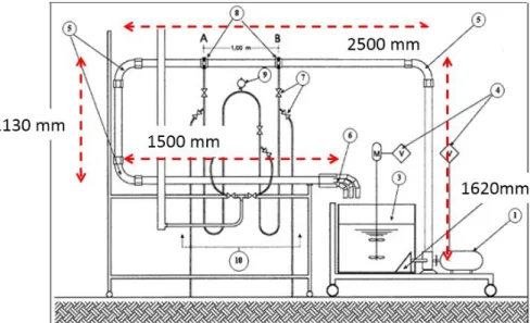
The solution domain used in this paper has the dimensions showed in figure 1, based on the experimental setup used by Pinto et al (2014). The pipe has an internal diameter of 50.1mm. The physical domain was discretized in a numerical model, for which four hexahedral meshes were created (Table 1).

(7)

Braz. J. of Develop., Curitiba, v. 5, n. 10, p. 20462-20477, out. 2019. ISSN 2525-8761 Table 1: Produced mesh

Mesh Number of elements

1 250560

2 443700

3 794952

4 1841856

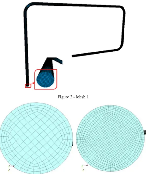
Figure 2 shows the mesh representing the flow domain in the pipe from the inlet to the outlet and figure 3 shows the differences between the coarsest and most refined meshes.

Figure 2 - Mesh 1

Figure 3 - Comparation between mesh 1 (left) and mesh 4 (right)

3.2 FLUID MODEL

The fluid used in this simulation was a mixture of 12% in volume of apatite and water, containing particles of 249 to 297 micrometers of granulometry. Two different models for viscosity

(8)

were used in the simulation, the constant equivalent viscosity model and the variable viscosity model.

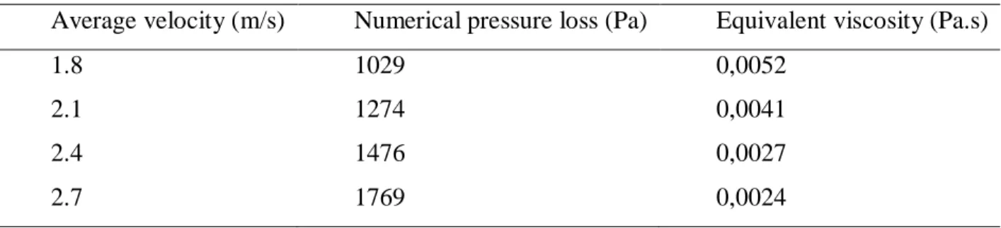
For the first method, to evaluate the equivalent viscosity, the experimental results produced by Souza Pinto (2014) were used. These values and the resulting equivalent viscosity are listed in table 2, for different values of average velocity.

Table 2: Equivalent viscosity for each average velocity

Average velocity (m/s) Numerical pressure loss (Pa) Equivalent viscosity (Pa.s)

1.8 1029 0,0052

2.1 1274 0,0041

2.4 1476 0,0027

2.7 1769 0,0024

The specific mass of the mixture was also given in the paper, which is 1257kg/m³.

For the second method, the same experimental data of pressure loss were used to determine the parameters k (consistency index) and n (behavior index). In this case, it was used the methodology described by Laun (1983), because for non-Newtonian fluids the shear stress on the wall is not proportional to the strain rate using the equivalent viscosity. The author suggests using the shear stress calculated at 83% of the radius and the ratio between this value and the equivalent viscosity as the real strain rate. With these values, a curve can be interpolated to find k and n.

Figure 4 shows the curve interpolating the data. The values found were 0.504 for k and 0.363 for n, with a R² of about 0.97.

(9)

Figure 4 – Adjusted curve

3.3 BOUNDARY CONDITIONS

The boundary conditions applied in this model were the same used for Souza Pinto (2014), which made it possible to compare the numerical analysis to the experimental results. The average velocities applied to the pipe inlet were the values listed in table 2. Because 1.3m/s is below the critical velocity, this case was excluded from the study. In the pipe outlet, it was used null relative pressure, and, at the walls, a no slip condition. The turbulence model used was k-ε.

The machine used had an intel i7 processor of 3.4Ghz; 32Gb of RAM of 1600Mhz; 120GB SSD and 3Gb DDR5 video card.

3.4 NUMERICAL UNCERTAINTY

Because the meshes generated were unstructured, the nodes were not coincident. To calculate the uncertainty at all nodes of the mesh, a python algorithm was developed, where the results of two meshes were interpolated in a linear way using the average of the four nearest nodes (Because the mesh is totally hexahedral, any node in the same domain will always be closer to one face).

After obtaining the interpolated results, the errors and percentage of errors were calculated in relation to the refinement of the mesh defining the uncertainty in the entire geometry.

(10)

4. RESULTS AND DISCUSSION

4.1 CONSTANT EQUIVALENT VISCOSITY

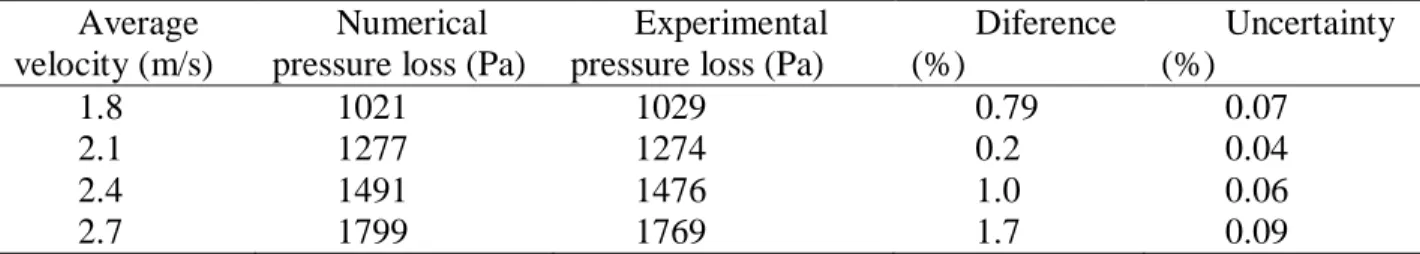
The results had a maximum difference of 1.7% when compared to the experimental data as shown in table 3.

Table 3: Numerical pressure losses versus Experimental pressure losses – Equivalent viscosity

Average velocity (m/s)

Numerical pressure loss (Pa)

Experimental pressure loss (Pa)

Diference (%) Uncertainty (%) 1.8 1021 1029 0.79 0.07 2.1 1277 1274 0.2 0.04 2.4 1491 1476 1.0 0.06 2.7 1799 1769 1.7 0.09

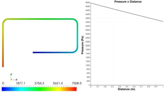
Figure 5 shows the pressure field and the pressure curve of the mathematical model for the case of 1.8 m/s. The pressure curve was measured in the same region of interest used by Souza Pinto

(2014) in the experiment.

Figure 5 – Numerical pressure results with average velocity of 1.8m/s

For this model, the highest differences between the numerical solution and experimental data were expected to be found at the critical velocity of 1.8 m/s because the equivalent viscosity model is not valid for velocities lower than the critical one. However, the methodology was more accurated in low-flow than in high-flow pumping, observing that the difference increases as the flow velocity increases.

(11)

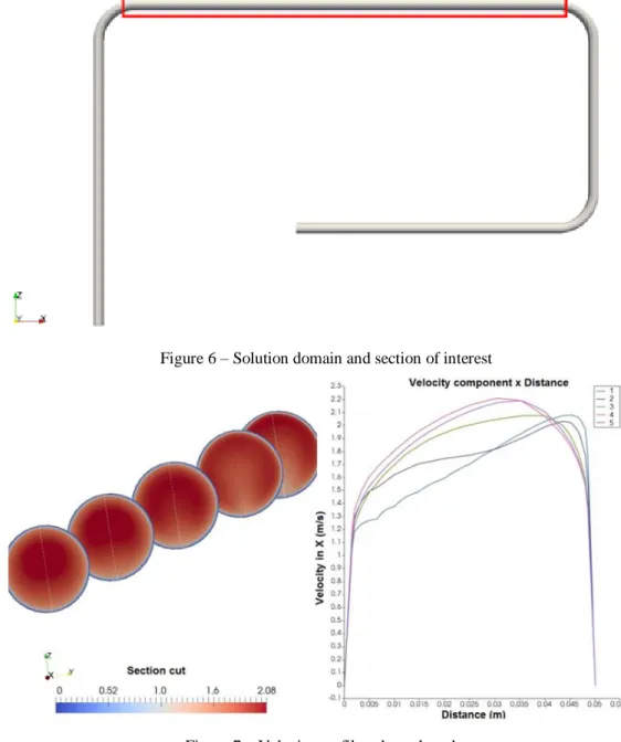
Figure 7 shows the x-velocity along several sections of the pipe from the end of the 90º knee to the end of the section of interest (Figure 6). Dividing this region in 4 equal parts, the velocity profile variation did not exceed 1% in the last part, indicating that the flow could be assumed was fully developed.

Figure 6 – Solution domain and section of interest

Figure 7 – Velocity profiles along the tube

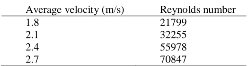
To verify the flow regime, the Reynolds number was calculated for each case, verifying that for values above the critical velocity the flow is turbulent (Reynolds greater than 2300). The values obtained are shown in Table 4:

(12)

Braz. J. of Develop., Curitiba, v. 5, n. 10, p. 20462-20477, out. 2019. ISSN 2525-8761 Table 4: Reynolds number

Average velocity (m/s) Reynolds number

1.8 21799

2.1 32255

2.4 55978

2.7 70847

To determine the uncertainty, the meshes 1, 2 and 3 of Table 1 were used. The difference between the results of the coarsest mesh to the most refined mesh was determined. Because this difference was smaller than 0.09% the results of the coarsest mesh was used.

To evaluate the uncertainty for the 2.1m/s case in the section of interest (Figure 6), the nodes interpolation algorithm for mesh 1 was applied. The results obtained are shown in Figure 8.

Figure 8 – Uncertainty results in section of interest

4.2 VARIABLE VISCOSITY

The variable viscosity model using the most refined mesh (mesh 4) was applied to calculate the pressure loss along the pipe. The difference between the numerical solution and the experimental results did not exceed 9.47% (Table 5). As expected, the greatest difference between these results was in the critical velocity, which is the limit of application of the equivalent viscosity equation.

(13)

Braz. J. of Develop., Curitiba, v. 5, n. 10, p. 20462-20477, out. 2019. ISSN 2525-8761 Table 5: Numerical pressure losses versus Experimental pressure losses – Variable viscosity

Average velocity (m/s)

Numerical pressure loss (Pa)

Experimental pressure loss (Pa)

Difference (%) Uncertainty (%) 1.8 932 1029 9.47 0.04 2.1 1120 1274 5.84 0.14 2.4 1499 1476 1.59 0.25 2.7 1826 1769 3.22 0.00

It can be observed that the calculated values of the pressure loss are smaller than the experimental values for the 1.8 m/s and 2.1m/s flow velocities and higher than these values for the 2.4m/s and 2.7m/s flow velocities, which indicates that the divergence of the results increases for extrapolated values. However, it is possible to interpolate flow velocity values that are within the experimental range.

Figure 9 shows the pressure curve along the region of interest for the 1.8m/s case. The images corresponding to the other flow cases (2.1m/s, 2.4m/s and 2.7m/s) are similar.

Figure 9 – Numerical pressure results with average velocity of 1.8m/s

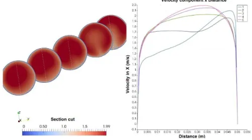
To evaluate if the flow is approaching to the fully developed condition, Figure 10 depicts the x-velocity along several sections of the pipe, from the end of the 90º knee to the end of the section of interest (Figure 6). The result in this case was similar to that of item 4.1, where in the last 25% of the region length the difference between the velocity profiles was approximately 1%.

(14)

Braz. J. of Develop., Curitiba, v. 5, n. 10, p. 20462-20477, out. 2019. ISSN 2525-8761 Figure 10 – Velocity profiles along the section of interest

To calculate the uncertainty, the meshes 2,3 and 4 of Table 1 were used, with the best results being those obtained through the mesh 4. For this calculation, the equation was used for the most refined mesh in relation to the coarsest mesh. Even with a greater refinement of the mesh, the variation of the results did not exceed 0.25%.

Evaluating the uncertainty result in the region of interest (Figure 6) in the domain highlighted in Figure 11 the highest uncertainty found in this section was 1.30%.

(15)

5. CONCLUSIONS

Two different methodologies - constant equivalent viscosity and variable viscosity - were tested to model a slurry flow, and their benefits and limitations were evaluated. The results showed that both methodologies can be used depending on the results expected from each modeling.

Equivalent viscosity modeling is more suitable in situations where there is a possibility of performing an experiment with the fluid. This type of modeling can be extended to any type of geometry as long as the flow rates are the same as the ones used in the experiment. This type of modeling did not require a refined mesh, and for the problem solved, differences smaller than 2% were found when compared to experimental data.

Variable viscosity modeling is independent of experimental results. Once the fluid is characterized, it is possible to replicate it to different geometries and different flow rates. The interpolation curve of the characteristic values of the fluid proved to be effective for interpolated values but indicated divergence for extrapolated values. This type of modeling required very refined meshes due to the high viscosity gradient between the elements of the mesh, where the difference between numerical results and experimental data did not exceed 10%.

Both constant viscosity and variable viscosity modeling, based only on the CFD technique, were not able to predict the fluid behavior below the critical velocity.

ACKNOWLEDGMENTS

The authors generously acknowledge the support of PUC Minas, FAPEMIG and National Council for Scientific and Technological Development (CNPq).

This study was financed in part by the Coordenação de Aperfeiçoamento de Pessoal de Nível Superior – Brasil (CAPES) – Finance Code 001

REFERENCES

Bijjam, S., Dhiman, A.K., 2012. Cfd analysis of two- dimensional non-newtonian power-law flow across a circular cylinder confined in a channel. Chemical Engineering Communications, 767–785. Blais, B.L., M., G., C., F., L., B., F., 2016. Development of an unresolved cfd–dem model for the flow of viscous suspensions and its application to solid–liquid mixing. Journal of Computational Physics 318, 201–221.

Dabirian, R., Mohan, R.S., Shoham, O., 2017. Mechanism modeling of critical sand deposition velocity in gas-liquid stratified flow. Journal of Petroleum Science and Engineering 156, 721-731.

(16)

Durand, R., 1952. The hydraulic transportation of coal and other materials in pipes. Board, London. Frigaard, I.A., Paso, K.G., Souza Mendes, P.R., 2017. Bingham’s model in the oil and gas industry. Rheologica Acta, 56, 3, 259-282.

Gopaliya, M.K.K., R, D., 2016. Modeling of sand-water slurry flow through horizontal pipe using cfd. Journal of Hydrology and Hydromechanics 64, 261–272.

Januário, J.R., Maia, C.B., 2020. CFD-DEM simulation to predict the critical velocity of slurry flows. Journal of Applied Fluid Mechanics, Vol. 13, No. 1, pp. 161-168

Min, F., Song, H., Zhang, N., 2018. Experimental study on fluid properties of slurry and its influence on slurry infiltration in sand stratum. Applied Clay Science 161, 64-69.

Souza Pinto, T.C., Junior, D.M., Slatter, P.T., Filho, L.S.L., 2014. Modelling the critical velocity for heterogeneous flow of mineral slurries. International journal of multiphase flow 65, 31–37. Singh, M.K., Kumar, S., Ratha, D., Kaur, H., 2017. Design of slurry transportation pipeline for the flow of multi-particulate coal ash suspension. International Journal of Hydrogen Energy 42, 30, 19135-19138.

Turian, R.M., Hsu, F.L., Ma, F.L.G., Sung, M.D., Plack- man, G.W., 1998. Flow of concentrated non-newtonian slurries: 2. friction losses in bends, fittings, valves and venturi meters. International Journal of Multiphase Flow 24, 243–270.

Turian, R.M., Hsu, F.L.G., Ma, T.W., 1987. Estimation of the critical velocity in pipeline flow of slurries. Powder Technology 51, 35–47.

Versteeg, H.K.M., Weeratunge, 2007. An introduction to computational fluid dynamics: the finite volume method. Pearson Education.

WAHBA, E.M., 2013. Non-newtonian fluid hammer in elastic circular pipes: Shear-thinning and shear- thickening effects. Journal of Non-Newtonian Fluid Mechanics 198, 24–30.

Warsi, Z.U., 2005. Fluid dynamics: theoretical and computational approaches. CRC press.

Wasp, E.J., Slatter, P.T., 2004. Deposition velocities for small particles in large pipes. Prague, Czech Republic

Yang, D., Xia, T., Wu, D., Cheng, P., Zeng, G., Zhao, X., 2018. Numerical investigation of pipeline transport characteristics of slurry shield under fravel stratum. Tunnelling and Underground Space Technology 71, 223-230.

(17)