Estud. Econ. vol.33 número3

1850 to 2000: An Empirical

Investigation

Eurilton Araujo

Ibmec Business School

Alexandre Cunha

Ibmec Business School

RESUMO

A possibilidade de que políticas de combate à inflação possuam efeitos negativos sobre a atividade econômica real e o crescimento é um assunto recorrente no Brasil. Neste traba-lho foram utilizados dados anuais para se estudar o comportamento da inflação e do PIB brasileiro de 1850 até 2000. Adotaram-se técnicas econométricas e da literatura de ciclos econômicos para se estudar o comportamento dessas duas variáveis nos domínios do tempo e da freqüência. Os resultados sugerem que as duas séries não são positivamente relacio-nadas. Assim sendo, a evidência empírica aparentemente indica que a opção de abrandar a política de combate à inflação com intuito de não prejudicar a atividade econômica real e o crescimento não está disponível para os condutores da política econômica brasileira.

PALAVRAS-CHAVE

inflação, crescimento, ciclos econômicos

ABSTRACT The question of whether a policy that leads to low inflation can hamper real economic activity and growth is a recurrent one in Brazil. In this essay we used yearly data to study the behavior of Brazilian inflation and GDP from 1850 to 2000. We used econometric and business cycles techniques to study the behavior of these variables in time and frequency domains. The results suggest the absence of positive comovement between the series. Thus, the empirical evidence apparently implies that the option of easing up on inflation to avoid a slowdown in real economic activity and growth is not available to Brazilian policy makers.

KEY WORDS inflation, growth, business cycles

INTRODUCTION

The question of whether a policy that leads to low inflation can hamper real economic activity and growth is a recurrent one in Brazil. This paper studies the empirical evidence on that issue. We use yearly data of inflation and GDP from 1850 to 2000 to investigate the joint behavior of these variables.

A didactical exposition of the view that stabilization policies may have long run negative effects on GDP is found in chapter 4 of Barbosa (1983). This author summarizes what became known as the estruturalista view of the inflationary process in Latin American economies.

Several authors advocate that there is some type of trade-off between inflation and growth in the long run. Prebisch (1968) states that “…given the economy structural vulnerability, the monetary stability is often not compatible with preserving the economic activity if the exports fall; the stability will induce a real contraction and to oppose to such a contraction will lead to inflation …”.1

Furtado (undated) shares Prebisch’s concerns. The former says that “The stability is a major goal, but it must be subordinated to a more important one, the development. An structural inflation, as the Brazilian one, to be defeated without harming development’s pace, demands a carefully planning of this last one.”2

In a recent work, Leite (2002) argues that the international experiences shows that there is some trade-off between inflation and growth. According to him, “I do not wish to resuscitate the old theory that some inflation may

1 Page 154. In Portuguese, “…dada a vulnerabilidade estrutural da economia, a estabilidade monetá-ria costuma ser incompatível com a manutenção da atividade econômica, quando as exportações decaem; a estabilidade leva à contração da economia, e opor-se a esta contração conduz geralmente à inflação…” The translation to English is ours. The same procedure will be adopted for the remaining quotations.

promote economic growth. However, it is necessary to admit that a growth acceleration will often push elements that will be translated into inflationary impulses.”3 _{He also states “What arises from the empirical evidence, as the major}

doubt in the formulation of a transition policy, is the apparent incompatibility between an acceleration in the growth pace that take us to the necessary level, soul of such a policy, and the prevalence of a monetary policy as tight as the one of a developed country, as it has been followed in Brazil.”4

Other authors also discuss the trade-off between growth and inflation. We refer the interested reader to Rangel (1978) and Thweatt and Kanitz (1967) for further discussions on this issue.

Prebisch (1968) argues that the views of himself and other estruturalistas on the relation between development and inflation are often misunderstood. He explicitly states that they are not biased towards the view that inflation may help economic growth.5 _{We are not aimed at identifying who did and} who did not say that inflation and development are related in some positive fashion. Our goal is to document that there existed and still exists a belief that there is some trade-off between inflation and economic growth.

We used several techniques to look into the properties of inflation and GDP series. None of them suggested that inflation and GDP are positively related in a sensible way.

The findings of this study have a policy implication. Namely, the empirical evidence suggests that the option of easing up on inflation to foster economic activity and growth on the long run does not seem to be available to Brazilian policy makers.6

3 Page 294. In Portuguese, “Não pretendo ressuscitar antiga tese de que um certo grau de inflação tenha efeito favorável na promoção do crescimento. Mas é necessário reconhecer que o fortalecimento do ritmo de crescimento resulta freqüentemente em pressões sobre fatores que se traduzem em impulsos infla-cionários.”

4 Page 294. In Portuguese, “O que surge da evidência empírica, como principal questionamento na formulação da política de transição, é a aparente incompatibilidade entre a aceleração do ritmo de cres-cimento que nos leve ao patamar necessário, essência dessa política, e a prevalência da política monetária com o rigor de país desenvolvido, que até aqui vem sendo seguida no Brasil.”

5 Page 128.

Our findings are fully consistent with other studies. Gosh and Phillips (1998) studied the relation between inflation and growth for several IMF members countries over the period 1960-1996. They concluded that, at very low inflation rate (2-3% per year), inflation and growth are positively correlated. Otherwise, inflation and growth are negatively correlated.

Kiguel and Liviatan (1992) and Végh (1992) found evidence that countries that adopted exchange rate based stabilization programs experienced an economic boom after a large fall in inflation rates. Thus, the empirical evidence does not necessarily corroborate the standard textbook trade-off between inflation and GDP of a Phillips curve. So, it should not be surprising that the actual Brazilian times series of inflation and economic activity do not behave in a textbook fashion.

This paper is organized as follows. In section I we provide a brief description of the joint evolution of inflation and GDP. In section II we carry out an econometric analysis of the series of inflation and GDP growth. Section III concludes. In the appendix (section IV) we describe our data set.

I. INFLATION AND THE BRAZILIAN BUSINESS CYCLES

A time series {x_t} can be decomposed into a trend component { T t

x

} and a

cyclical component { C t

x

} that satisfy

x

_t

=

x

T_t

+

x

_tC. There exist several ways

of decomposing {x_t}. Each of these possible decompositions is linked to a definition of trend.

In this section the time series {y_t} of the log of the real GDP and the time series of {p_t} of the log of the price level will be decomposed into cyclical and trend components. The well-known Hodrick-Prescott (HP) decomposition will be used. The smoothing parameter λ will be set equal to 100.7

The difference C t C

t

p

p

−

−1 is defined here as the cyclical component C t

π

of the inflation rate. Observe that this procedure amounts to first filter the series of price and then compute trend and cyclical inflation rates. It would be possible to first evaluate the inflation rate πt and then decompose it with

the Hodrick-Prescott filter. The two procedures do not generate exactly the same series for T

t

π

and C t

π

. However, it turned out that, except for the end points of the sample, the resulting series are very similar. Thus, the qualitative conclusions presented in this essay do not depend on which of the two procedures is adopted.

I.1 The Brazilian GDP from 1850 to 2000

The time series {y_t} and { T t

y

} are plotted in Figure 1, while { C t

y

} is plotted

in Figure 2. A striking feature is the acceleration of the trend component that took place by the end of the 1800’s and its subsequent slowdown at the beginning of the 1980’s.8

The most surprising feature of the cyclical behavior of the GDP is the strong 1890-1892 boom, the deep 1893-1894 recession and the strong recovery in 1895. According to Goldsmith (1986), a bank liberalization that took place with the advent of the Republic in 1889 triggered the boom and a subsequent general banking crisis caused the ensuing recession. This period corresponds to the well-known encilhamento.9

8 As explained in the appendix, we linked two distinct GDP series in 1901 to construct a series for the entire 1850-2000 period. This procedure is not responsible for the aforementioned acceleration. The break in the trend component of the GDP takes place in 1895 and not in 1901. Both BAER (1996) and PRADO JR. (1979) stated that an industrial surge started in the 1880’s. Additional evidence on that industrial take-off is provided in IBGE (1990). The industrial machinery and equipment imports data provided at table 7.6 of that book also displays a boom after 1880. It is well known that industrialization is often accompanied by rise in GDP’s growth rate. For evidence on this growth stylized fact, see BALDWIN, MARTIN & OTTAVIANO (1998). Thus, our GDP series is consistent with the available evidence on Brazilian economic history and the international experience.

The 1890-1895 cycle was by far the strongest one experienced by the Brazilian economy. Even the 1929 crisis and subsequent recovery did not have the same amplitude. In more recent years, the 1970’s were a time in which GDP was consistently above the trend.

FIGURE 1 - ACTUAL AND TREND LOGS OF ANNUAL GDP

I.2 The Brazilian Inflation from 1850 to 2000

The time series of πt and C t

π

are plotted in Figure 3. The period from 1850 to 1950 was a period in which the trend was relatively stable and near to zero. After 1950 the trend was positive and increasing up to 1990. After that year the trend was clearly decreasing.

FIGURE 3 - ACTUAL AND TREND INFLATION

I.3 Cross Correlations of the Cyclical Components of GDP and Inflation

The cross correlations of C t

TABLE 1 - CROSS CORRELATIONS OF C t

y

WITH

π

tC−j

j \ periods 1851-2000 1851-1889 1890-1930 1931-1945 1946-1963 1964-1984 1985-2000 0 -0.0476 -0.1327 0.1885 -0.0333 0.1239 0.2665 -0.3919 1 -0.0866 -0.0245 -0.2488 0.1419 -0.1188 0.0231 -0.2818 2 -0.1264 0.0766 -0.4621 0.3741 -0.4059 -0.1868 -0.2948 3 -0.0524 0.1284 0.0604 0.1968 -0.4063 -0.3589 -0.0859 4 0.0065 0.1979 0.2036 0.4849 -0.3988 -0.2784 0.1764 5 0.0483 0.2894 0.2628 -0.2069 -0.2063 -0.1692 0.3730 6 0.0432 0.1350 0.0487 -0.2273 0.0735 -0.2424 0.5416 7 0.0121 0.0639 -0.1446 -0.4031 0.1443 -0.3345 0.5400 8 -0.0328 -0.2427 -0.1648 -0.9127 0.4587 -0.1839 0.2626 9 -0.0207 -0.4163 0.0648 -0.0811 0.1701 0.0063 -0.6669

For the period 1851-2000, C t

y

is correlated in a negative way with

π

_tC

and its first three lags, in a positive way with lags four to seven and again in a negative way with the last two lags. No general pattern is found when the cross correlations are evaluated over sub-periods.

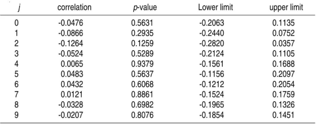
Table 2 displays confidence intervals and p-values for the 1851-2000 period cross correlations. Figure 4 displays the correlogram of C

t

y

and

π

tC−j. It

was assumed that ( , C )

j t C t

y π ₋ is asymptotically normal to compute the p

-values and confidence intervals.

TABLE 2 - CROSS CORRELATIONS OF C t

y

WITH

π

tC−j 95%

CONFIDENCE INTERVALS AND P-VALUES

j correlation p-value Lower limit upper limit

0 -0.0476 0.5631 -0.2063 0.1135

1 -0.0866 0.2935 -0.2440 0.0752

2 -0.1264 0.1259 -0.2820 0.0357

3 -0.0524 0.5289 -0.2124 0.1105

4 0.0065 0.9379 -0.1561 0.1688 5 0.0483 0.5637 -0.1156 0.2097 6 0.0432 0.6068 -0.1212 0.2054 7 0.0121 0.8861 -0.1524 0.1759

8 -0.0328 0.6982 -0.1965 0.1326

FIGURE 4

None of the correlations are significant at 5%. The lower limits of the confidence interval are all negative, while the upper ones are all positive. There is no evidence of a high degree of positive comovement between C

t

y

and C j t−

π

.

I.4 Granger Causality Tests

In this section it is studied whether the cyclical component of the inflation

rate ( C t

π

) Granger-causes the cyclical component of output ( C t

y

), as well

as whether C t

y

Granger-causes

π

_tC.

To verify whether C t

π

Granger-causes C t

y

, equations

t k j C j t j C t

y

y

=

α

+

∑

β

+

ε

=1 −

(1)

and t k j C j t j k j C j t j C t

y

y

=

α

+

∑

β

+

∑

γ

π

+

ε

= − =1 − 1

are estimated by ordinary least squares (OLS). Then, the null hypothesis

γ₁ = γ₂ =…= γ_k = 0 is tested. Let RSS₁ and RSS₂ denote, respectively, the sum of the squared residuals of regressions (1) and (2). A possible way to test the null hypothesis is to evaluate the statistic

2 2 1

)

)(

1

2

(

RSS

RSS

RSS

k

T

S

=

−

+

−

(3)

where T is the number of usable observations. S has a Chi-square distribution with k degrees of freedom.

The procedure to check whether C t

y

Granger-causes C t

π

is similar to the one just described. In fact, it amounts to estimating equations

t k j C j t j C

t

α

β

π

ε

π

=

+

∑

_{=1 −}

+

and t

k j C j t j k j C j t j C

t

α

β

π

γ

y

ε

π

=

+

∑

_{=1 −}

+

∑

_{=1 −}

+

by OLS. Then, the S statistic defined in (3) is evaluated.

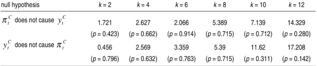
According to the Akaike information criterion (AIC), the lag length k is equal to 12. The Hannan-Quinn Criterion (HQC) specifies k = 8, while the Schwarz Information Criterion (SIC) dictates k = 2. We carried out the Granger causality testes for these three and some other values of k. The results are summarized next.

TABLE 3 - GRANGER CAUSALITY TESTS – VALUES OF S AND P-VALUES

null hypothesis k = 2 k = 4 k = 6 k = 8 k = 10 k = 12

C t

π does not cause y_tC _{1.721 2.627 2.066 5.389 7.139 14.329}

(p = 0.423) (p = 0.662) (p = 0.914) (p = 0.715) (p = 0.712) (p = 0.280)

C t

y does not cause π_tC _{0.456 2.569 3.359 5.39 11.62 17.208}

(p = 0.796) (p = 0.632) (p = 0.763) (p = 0.715) (p = 0.311) (p = 0.142)

The null hypothesis was not rejected at each of those tests. So, the evidence

does not suggest that either

π

tC Granger causes C t

y

or

y

_tC Granger causes

I.5 Summary of the Findings

This section investigated the joint behavior of the cyclical components of inflation ( C

t

π

) and GDP ( C t

y

). The observed cross correlations of

y

C_t

with C t

π

and its lagged values are not consistent with the notion that a decrease in the inflation rate should be accompanied by a decrease in output. No evidence that C

t

π

Granger-causes C t

y

was found either. The available

evidence seems to speak against the possibility of using inflation as a policy tool to stimulate economic activity.

II. THE COMOVEMENT BETWEEN GDP GROWTH AND

INFLATION

This session focus on the relationship between GDP growth and inflation. We employ time series techniques to analyze the comovement patterns of our two series in the long run as well as in the short run.

The view that inflation may grease the wheel of economic growth, in spite of the benefits of price stability, is still widely accepted in some economic policy circles. If this is the case, one should find evidence that inflation and output growth are positively related, either in short or long run.

To capture the notion of short and long run, we employ spectral analysis and study measures of feedback between the two series in the frequency domain. These measures are defined in Geweke (1982). We also compute the correlation between the two series over short and long horizons, using a methodology developed by Den Haan (2000).

II.1 The Empirical Techniques

a) Frequency Domain Analysis

Before starting the discussion on frequency domain techniques, it is important to stress that any feature of the data can be described by the time domain as well as by the frequency domain representation. For some features the time domain representation may be simpler while for other features the frequency domain description may be more appropriate.

In this section the relationship between two time series over different horizons is going to be considered. Frequency domain representation describes the data as the sum of components associated with cycles of different periodicities. Therefore, it allows for prompt recognition of cyclical components responsible for long, medium and short run behavior. So, the separation of long, medium and short run is easier to carry out in that domain.

The next few paragraphs contain a brief introduction to spectral representation. We present the basic concepts needed for the understanding of the econometrics used in this section.

Any time series {xt} can be represented by its spectral density, which is

∑

+∞ −∞ =

−

=

k x

x

k

i

k

f

(

)

exp(

)

2

1

)

(

γ

ω

π

ω

_{, where}

γ

(

k

)

is the auto-covariance

function of order kand the letter i denotes the complex number unit. The

spectrum is just the Fourier transform of auto-covariance functions.

In the bivariate case, the cross-spectrum is

∑

+∞ −∞ =

−

=

k xy

xy

k

i

k

f

(

)

exp(

)

2

1

)

(

γ

ω

π

ω

,

where

γ

_xy

(

k

)

is the cross-covariance

function of order k. The Greek letter

ω

denotes the angular frequency

associated with cycles of periodicity

2

_ω

π

.

and b such that the cross-spectrum can be written as

)

(

)

(

)

(

ω

a

ω

ib

ω

f

_xy

=

+

.

The function

a

(

ω

)

is called co-spectrum and

b

(

ω

)

is known as quadrature spectrum. The co-spectrum is the portion of the covariance between the two series considered attributable to cycles associated with the frequency

ω

. The quadrature spectrum measures covariance induced by out-of-phase cycles. A plot of the cross-spectrum of two time series provides a decomposition of the overall dynamic between the series by separating short and long run components.

It is worth noticing that cycles of a given frequency

ω

may be important for both series individually but may fail to account for the contemporaneous covariance between the two variables because at any given date the series may be in a different phase of the cycle.

The spectrum and the cross-spectrum can be estimated non-parametrically, using Kernel smoothing methods. For instance, consider the univariate process {x_t}. Its sample periodogram, which is the sample analogue of

)

(

ω

x

f

, is computed according to

)

exp(

)

(

ˆ

2

1

)

(

ˆ

1 1

iwj

j

f

T T j x

x

=

∑

−

− + − =

γ

π

ω

where each

γ

ˆ

_x

(

j

)

is a sample auto-covariance functions based on a sample of T observations, satisfying the condition

γ

ˆ

_x

(

l

)

=

γ

ˆ

_x

(

j

)

for

l

=

−

j

.

A Kernel estimator averages the sample periodogram over different

frequencies and can be constructed as

(

,

j

)

ˆ

x

(

j m

)

h h m m j

f

k

₊ − = +

∑

ω

ω

ω

_{. The}

Ha-milton (1994) recommended the use of the Kernel 2

)

1

(

1

)

,

(

+

−

+

=

+

h

m

h

k

ω

_{j m}

ω

_j .

A useful measure of linear correlation between two components of a bivariate process at a given frequency is called coherence, which is a frequency domain analogue of the R2 of basic regression analysis. Coherence

can be computed using the following formula:

)

(

)

(

)

(

)

(

)

(

2 2

ω

ω

ω

ω

ω

y x

f

f

b

a

C

=

+

₍₄₎

Note that

a

(

ω

)

and

b

(

ω

)

are the co-spectrum and the quadrature spectrum,

which have already been defined in this paper, while

f

x

(

ω

)

and

f

y

(

ω

)

are

the spectrum of individual components of the bivariate process and C(ω) is the coherence. It can be shown that (4) implies that

0

≤

C

(

ω

)

≤

1

.

b) Feedback Measures

Geweke (1982) defines linear feedback measures for multivariate time series and decompose these measures frequency by frequency. This decomposition can be viewed as Granger-causality measures in the frequency domain. These measures capture the notion that past values of a particular time series may help to forecast other series in a multivariate system.

The measure proposed by Geweke is constructed as follows. First consider the equations: t s t s s s t s s

t

E

x

F

y

u

x

₂

1 2 1

2

+

+

t s t s s s t s s

t

H

x

G

y

v

y

₃

1 3 1

3

+

+

+

=

∞ ₋ = − ∞ =

∑

∑

δ

_{. (6)}

The process {xt} can be represented as

x

t

=

P

(

L

)

u

2t

+

Q

(

L

)

v

3t. The

functions P(L) and Q(L) are polynomials in the lag operator L.

Let

T

3be the variance of

v

3tand let

Σ

2 be the variance for

u

2t. Observe

that

v

3t can be interpreted as new information entering the system at a

given time due to y_t rather than to x_t. The spectral density of {x_t} at a frequency

ω

can be written as:

)

(

~

)

(

~

)

(

~

)

(

~

)

(

ω

P

ω

₂

P

'

ω

Q

ω

T

₃

Q

'

ω

S

_x

=

Σ

+

, (7)

where the “~” sign denotes Fourier transform of the indicated lag operator.

The measure of feedback

f

Y→X

(

ω

)

from {yt} to {xt} at frequency

ω

is

defined as

















Σ

=

→

)

(

~

)

(

~

ln

)

(

' 2

ω

ω

ω

P

P

S

f

_{Y X} x _{. (8)}

This non-negative measure indicates the relative importance of the contributions of

T

3, the variance of

v

3t, and

Σ

2, the variance for

u

2t, to

the variance of {x_t} at a given frequency. It will approach infinity as the relative importance of the variance in the innovation associated with {y_t} to the variance of {xt} increases at the frequency considered. This measure

feedback from {yt} to {xt}. Of course, an analogue measure of feedback

from {x_t} to {y_t} can be built.

c) Measures of Comovement over Different Horizons

Den Haan (2000) proposed the following measures of comovement between two series. The first measure consists in computing the correlation of the two series at different forecast horizons. The second consists in filtering the two series using the band-pass filter proposed in Baxter and King (1999). We next detail the two procedures.

The initial step in computing the first measure is to estimate a vector auto-regressive representation for the bivariate process. After that the K-period ahead forecast error is computed, whenever possible, for each observation of the time series being studied. The correlation between the forecast error series associated with each variable in the system can be computed for a given K. So, it is possible to evaluate these correlation coefficients as a function of the forecast horizons K. If the series are stationary, the correlation coefficients of the forecast errors will converge to the unconditional correlation coefficient of the two series as K increases.

Let GDP growth and inflation be denoted by

∆

y

t and

π

t. The vector

process can be written as











∆

=

t

π

t t

y

X

_.

The process {X_t} can be put in the VAR framework

t l t L

l l

t

g

t

A

X

e

X

=

+

₋

+

=

∑

1

)

(

_{. The function}

_g

₍

_t

₎

_{denotes some deterministic}

The K period ahead forecast errors are: , t K t

(

t K

)

y t K

t

y

E

y

e

∆₊

=

∆

₊

−

∆

₊ and

)

(

,t t K t t K K

t

E

e

π₊

=

π

₊

−

π

₊ , while the correlation coefficient corr(K) of the forecast errors is given by

)

(

std

)

(

std

)

,

cov(

)

(

, , , , π π t K t y t K t t K t y t K t

e

e

e

e

K

corr

+ ∆ + + ∆ +

=

₍₉₎

The symbols cov and std denote, respectively, covariance and standard deviation.

The second measure of comovement proposed by Den Haan (2000) uses the Baxter and King filter. A filter is able to isolate specific frequency bands, associated with cycles characterized by a given periodicity. The Baxter and King filter is a two-sided symmetric smoother designed to approximate the ideal band-pass filter. Any series, after filtered, can be represented as

t F

t

B

L

x

x

=

(

)

, where the polynomial B(L) is given by h

h h

L

b

L

B

∑

+∞ −∞ =

=

)

(

, with

h

h

b

b

=

₋ .

The ideal band-pass filter is an infinite moving average. The weights b_h can

be computed according to

π

1 2 0

f

f

b

=

−

and

h

h

f

h

f

b

_h

π

)

sin(

)

sin(

₂

−

₁

=

for

,...

3

,

2

,

1

±

=

h

The specified frequency band is given by

[

f

2

,

f

1

]

.

Baxter and King (1999) proposed an approximate band-pass filter and showed how to compute the weights. Their filter may be written as

h H H h h

L

a

L

A

∑

+ − =

=

)

(

. The weights are

a

_k

=

b

_k

+

θ

. The parameter H is the

degree of truncation and

∑

+

− =

+

−

=

H H k

b

k

H

1

2

1

In this paper, GDP growth and inflation will be filtered in order to isolate cycles with periods of 2 years up to a specified periodicity associated with a frequency

ω

p. Hence, we will be able to plot the correlation associated

with the band

[

ω

p,

π

]

against the periodicity implied by the frequency

ω

p.

II.2 The Vector Auto-Regressive Process for Inflation and GDP Growth

It is necessary to estimate a VAR for inflation and GDP growth for the following reasons: First, one of the methods suggested by Den Haan (2000) is entirely based on a VAR representation for the bivariate process in question. Second, the VAR allows us to simulate the bivariate process in order to generate artificial time series, which are necessary elements in computing 95 per cent confidence bands by bootstrap. In this study we will compute confidence bands for the feedback measures proposed by Geweke and for correlation coefficients.

The time series for inflation shows an anomalous behavior from 1975 to 1994. This is not a surprise, since during the 1980’s high inflation was accompanied by unsuccessful stabilization plans that were followed by even higher levels of inflation. Therefore, the strategy for estimating the VAR for the entire sample period has to take into account this hyperinflation regime. Furthermore, the bivariate process will be estimated for different periods in order to assess the effects of considering the hyperinflation regi-me on our results.

possible to evaluate how robust our findings are to an episode of extreme economic prosperity. The same applies to the comparison of results for the first sample and for the whole period of analysis. But in this case, we are checking the robustness of our results to an episode of instability and very little economic growth.

The specifications for the first and second samples are presented in Tables 4 to 9. We allow for a linear and a quadratic deterministic trend in both specifications.

TABLE 4 - FIRST EQUATION - INFLATION IS THE DEPENDENT VARIABLE: 1850-1960 SAMPLE

Variable Coefficient t Statistics

Constant 0.043697 1.37702

Linear Trend -0.001485 -1.23382

Quadratic Trend _2.14×₁₀−5 _1.92412

Inflation (-1) 0.283798 2.90314

Inflation (-2) 0.038044 0.36583

Inflation (-3) -0.001212 -0.18374

Inflation (-4) -0.018605 -0.18374

GDP Growth (-1) 0.339425 1.88521

GDP Growth (-2) -0.083708 -0.46662

GDP Growth (-3) -0.091920 -0.51744

GDP Growth (-4) -0.540833 -3.06538

TABLE 5 - SECOND EQUATION - GDP GROWTH IS THE DEPENDENT VARIABLE: 1850-1960

Variable Coefficient t Statistics

Constant 0.053522 3.01591

Linear Trend -0.001117 -1.65963

Quadratic Trend 5

10 67 .

1 × − 2.67519

Inflation (-1) -0.069533 -1.27188

Inflation (-2) -0.073912 -1.27088

Inflation (-3) 0.098236 1.67769

Inflation (-4) -0.000986 -0.01742

GDP Growth (-1) -0.077128 -0.76600

GDP Growth (-2) -0.263579 -2.62726

GDP Growth (-3) -0.072612 -0.73089

The lags were chosen by looking at the AIC information criterion and by analyzing the residuals. To obtain a parsimonious model, the AIC criterion has to be minimized. In addition, the multivariate process for the residuals has to be a white noise. Therefore, the specification above is based on the minimization of the AIC criterion restricted to a set of specification which leads to white-noise-like residuals. In fact, although the inclusion of additional lags does not imply additional significant coefficients, it helps the generation of white-noise-like residuals. To check the residuals, we have employed a multivariate LM test to evaluate the presence of autocorrelation. Table 6 summarizes the results for this test.

TABLE 6 - BIVARIATE LM RESIDUALS TEST FOR SERIAL CORRELATION: 1850-1960 SAMPLE

Lags Test Statistic p-Value

1 5.137781 0.2735 2 4.634745 0.3269 6 2.562353 0.6335 9 1.949875 0.7450

12 2.33054 0.6752

We specify the VAR process for the second sample in the same way described before. Results are presented in Tables 7, 8 and 9.

TABLE 7 - FROM 1850 TO 1975 - FIRST EQUATION: INFLATION IS THE DEPENDENT VARIABLE

Variable Coefficient t Statistics

Constant 0.026182 0.99842

Linear Trend -0.001529 -1.58000

Quadratic Trend 5

10 87 .

1 × − 2.30092

Inflation (-1) 0.516139 6.42501

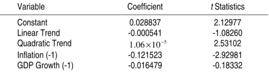
TABLE 8 - SECOND EQUATION – GDP GROWTH IS THE DEPENDENT VARIABLE: 1850-1975 SAMPLE

Variable Coefficient t Statistics

Constant 0.028837 2.12977

Linear Trend -0.000541 -1.08260

Quadratic Trend _1.06×10−5 _2.53102

Inflation (-1) -0.121523 -2.92981

GDP Growth (-1) -0.016479 -0.18332

TABLE 9 - BIVARIATE LM RESIDUALS TEST FOR SERIAL CORRELATION: 1850-1975 SAMPLE

Lags Test Statistic p-Value

1 6.545148 0.1620 2 7.205023 0.1254 6 1.481846 0.8299 9 3.392042 0.4945 12 6.131479 0.1895

The VAR specification for the whole period of analysis takes into account the break in the level of inflation. Figure 3 shows clearly that break, which is a result of high inflation rates and unsuccessful stabilization plans. In order to propose a VAR model for the entire sample, the first step is to identify a probable date for the break. Vogelsang and Perron (1998) discuss a methodology to identify a single break in a time series trend at an unknown time. Following this methodology, we focus on the Additive Outlier case, in which a break is assumed to occur instantly. The models for the trend of inflation allowing for a break are:

t t

t

µ

β

t

θ

DU

η

π

=

+

+

+

(

M

₁

)

t t t

t

µ

β

t

θ

DU

λ

DT

ξ

π

=

+

+

+

+

(

M

₂

)

t t

t

µ

β

t

λ

DT

ξ

where

DU

_t

=

I

(

T

_b

<

t

<

1995

)

and

DT

t

=

I

(

T

b

<

t

<

1995

)(

t

−

T

b

)

. The operator I(⋅) denotes the indicator function and T_b is the break date considered. Note that the break is over in 1995, since in 1994 the Real Plan, one of many stabilization plans launched by the Brazilian government, successfully curbed inflation.

The choice of the trend inflation model and the determination of T_b are based on a data-dependent method. First, for each model, T_b is chosen to maximize some statistic associated with the significance of one or more of the break parameters. Then, a model is chosen based upon goodness of fit criteria, such as log likelihood, AIC and Schwarz information criteria.

To implement the proposed method we proceed as follows. For model M₁,

T_b is chosen based on the maximum value for the t-statistic for

θ

ˆ

_{. For} model M₂, T_b is chosen based on the maximum value for the t-statistic for

λ

ˆ

_{. Alternatively, T}

b can be chosen based on the maximum value for the F

-statistic for testing the joint hypothesis

θ

=

λ

=0. For model M₃, T_b is

chosen based on the maximum value for the t-statistic for

λ

ˆ

_.

With a T_b chosen for each model, we compare models’ log likelihood, AIC and Schwarz information criteria. It turned out that M₃ is strictly better than the other two under log likelihood and Schwarz criteria, while the AIC criterion was not conclusive. Thus, we pick model M₃ and set T_b = 1980.

sensible statistical criterion. The procedure described in Vogelsang and Perron (1998) helps us accomplish our objective.

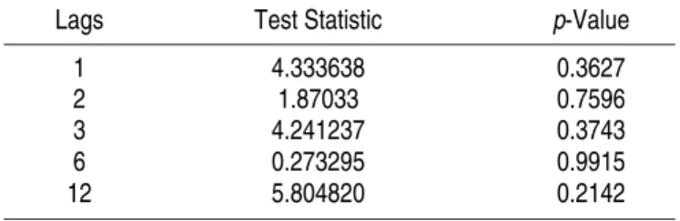
The specification for the VAR is summarized in Tables 10 to 12. Tables 10 and 11 show coefficients estimates for the VAR. Table 12 shows that the residual are white noise. It is worth remembering that the specification for the entire sample will be used in the following sub-sections to address the dynamic correlation between inflation and GDP growth.

TABLE 10 - FIRST EQUATION – INFLATION IS THE DEPENDENT VARIABLE: 1850-2000 SAMPLE

Variable Coefficient t Statistics

Constant -0.037463 -1.19314

Linear Trend 0.001392 3.14653

)

1980

(

_b

=

t

T

DT

0.157682 16.2164

Inflation (-1) 0.284904 4.61777

Inflation (-2) -0.117707 -2.35263

GDP Growth (-1) 0.455177 1.48178

GDP Growth (-2) 0.025237 0.08141

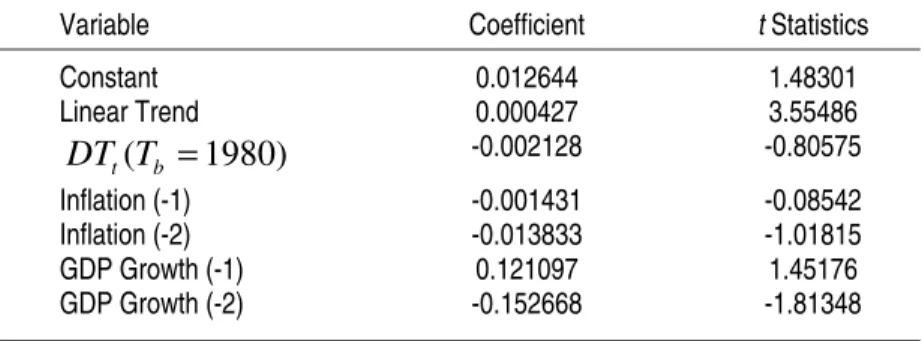
TABLE 11 - SECOND EQUATION – GDP GROWTH IS THE DEPENDENT VARIABLE: 1850-2000 SAMPLE

Variable Coefficient t Statistics

Constant 0.012644 1.48301

Linear Trend 0.000427 3.55486

)

1980

(

_b

=

t

T

DT

-0.002128 -0.80575

Inflation (-1) -0.001431 -0.08542

Inflation (-2) -0.013833 -1.01815

GDP Growth (-1) 0.121097 1.45176

TABLE 12 - BIVARIATE LM RESIDUALS TEST FOR SERIAL CORRELATION: 1850-2000 SAMPLE

Lags Test Statistic p-Value

1 4.333638 0.3627 2 1.87033 0.7596 3 4.241237 0.3743 6 0.273295 0.9915 12 5.804820 0.2142

II.3 Results

We plot below the measures of comovement discussed before, for three different samples. The first one goes from 1850 to 1960, the second covers the time period from 1850 to 1975. Finally, the last sample considers the whole period of analysis, i.e., from 1850 to 2000. The idea here is to isolate the effect of high inflation episodes, which affects strongly the data during the 1980’s and 1990’s.

All of the measures considered show that the series of inflation and GDP growth are not strongly related. Granger causality tests, in the frequency domain, offer some support to the existence of a linear relationship between inflation and output growth in the second sample. Finally, the effects of the “lost decades”(1980’s and 1990’s) are very strong. In these years, inflation was extremely high and the growth rate was small. In fact, when we consider the whole sample, all correlations are very low and Granger causality tests offer strong support to the non-existence of any consistent relationship between the two series.

FIGURE 5 - COHERENCE: 1850-1960 SAMPLE

FIGURE 7 - COHERENCE: 1850-2000 SAMPLE

Figures 8 to 10 shows feedback measures and also shows 95 per cent confidence bands constructed by bootstrap, after simulating the VAR 2500 times. The feedback measure from inflation to GDP growth cannot exceed 0.06 in the first sample. From 1850 to 1975, it cannot exceed 0.21. And finally, for the whole sample, the maximum feedback measure indexed by frequency is around 0.006.

Let φ(ω) denote the percentage of the variation in {x_t} explained by innovations in {y_t} at a given frequency ω. That variable is computed according to

)}

(

exp{

1

)

(

ω

ω

φ

=

−

−

f

Y→X

(10)

Again, there is some evidence that during the 1960’s and 1970’s inflation and GDP growth are more related. In the second sample, which includes the period 1960 to 1975, innovations associated with inflation are able to explain almost 20 per cent of the variation in GDP growth for some parti-cular frequency. In spite of that, 80 per cent of GDP growth cannot be attributable to inflation. Therefore, even in that sample the linear relationship between the series is weak.

The upper band related to the feedback measure from inflation to GDP growth is wider, especially in the low frequency range, in the second sample. This behavior is another evidence of an increasing, though weak, degree of relationship between the series.

In the third sample, the 1980’s and 1990’s contribute to make a possible weak relationship, existent in 1960’s and 1970’s, disappear. In fact, almost all the variation in GDP growth cannot be explained by inflation.

The upper band related to the feedback measure from GDP growth to inflation show that the maximum value for this measure is around 0.17 in the first sample, 0.19 in the second sample and 0.1 in the third sample. Thus, (10) implies that innovations associated with GDP Growth can explain at most 15.63 per cent of the variation in inflation in the first sample, 17.30 per cent of the variation in inflation in the second sample and finally 9.5 per cent of the variation in inflation in the third sample.

In short, the feedback measure from GDP growth to inflation tells a similar story in terms of a weak relationship in the second sample followed by an even weaker relationship. But now, the quantitative differences are less striking.

FIGURE 8 - GRANGER-CAUSALITY SPECTRAL DECOMPOSITION: 1850-1960 SAMPLE

FIGURE 10 - GRANGER-CAUSALITY SPECTRAL DECOMPOSITION: 1850-2000 SAMPLE

In each of the 2500 simulations, a set of artificial data was generated using the estimated VAR and random draws from a bivariate Normal distribution. Mean Corr stands for the mean of correlations across the 2500 replications performed. Realized Corr refers to the actual correlations, coming from the data.

Figures 11 to 13 and 14 to 16 show dynamic correlations, computed according to the two alternative methodologies suggested by Den Haan (2000). We also calculated 95 per cent confidence bands using bootstrap.

In the first set of figures, we plot the correlation of the VAR forecast errors. In the second one we plot the correlations of the data filtered by the Baxter-King band pass filter.

FIGURE 11 - VAR FORESCAST ERRORS CORRELATIONS: 1850-1960 SAMPLE

FIGURE 13 - VAR FORESCAST ERRORS CORRELATIONS: 1850-2000 SAMPLE

The dynamic correlation coefficients converge very fast to the unconditional correlation between inflation and GDP growth. None of the results change substantially when one uses filtered data to compute the dynamic correlations, as can be seen in Figures 14, 15 and 16 bellow.

FIGURE 15 - CORRELATIONS USING FILTERED DATA: 1850-1975 SAMPLE

III. CONCLUSION

There exists a recurring debate in Brazil on a possible trade-off between inflation and real economic activity and growth. This paper carried out an empirical investigation of the issue.

The sample consisted on yearly data, from 1850 to 2000, for both inflation and GDP in Brazil. Several statistical and econometric techniques were used to study the joint properties of the series. No strong evidence of a significant positive comovement between the two series was found. Though, there is some evidence that the linear relationship between the series increased from 1960 to 1975.

The findings of this study have a policy implication. Even if Brazilian policy makers were willing to ease up on inflation to stimulate economic growth, it does not seem reasonable to assume that such a policy would have a high probability of success

IV. APPENDIX: THE DATA SET

In Goldsmith (1986) we obtained series for nominal and real GDP from 1850 to 1901. We obtained at IPEADATA (http://www.ipeadata.gov.br) series for these two variables from 1901 to 2000. We combined the two sources to generate the series for nominal and real GDP from 1850 to 2000. The last series is our measure of real GDP. From those two series, we computed GDP’s implicit deflator and used it as our measure of price level.

REFERENCES

BAER, Werner. A economia brasileira. São Paulo: Nobel, 1996.

BALDWIN, Richard; MARTIN, Phillipe; OTTAVIANO, Gianmarco. Global income divergence, trade and industrialization: the geography of growth take-offs. National Bureau of Economic Research, Working

BARBOSA, Fernando. A inflação brasileira no pós-guerra. Rio de Janeiro: IPEA/INPES, 1983.

BAXTER, Marianne; KING, Robert. Measuring business cycles: approximate band-pass filters for economic time series. Review of

Economics and Statistics, v. 81, n. 4, p. 573-593, 1999.

DEN HAAN, Wouter; SUMMER, Steven. The comovements between real activity and prices in the G7. National Bureau of Economic Research, Working Paper 8195, 2001.

FURTADO, Celso. A política monetária. In: SÁ JR., Francisco (ed.),

In-flação e desenvolvimento. Petrópolis: Editora Vozes, undated.

GEWEKE, John. Measurement of linear dependence and feedback between multiple time series. Journal of the American Statistical Association, v. 77, n. 378, p. 304-313, 1982.

GOLDSMITH, Raymond. Brasil 1850-1984: desenvolvimento financeiro sob um século de inflação. São Paulo: Harper & Row do Brasil, 1986. GOSH, Atish; PHILLIPS, Steven. Warning: inflation may be harmful to

your growth. IMF Staff Papers, v. 45, n. 4, p. 672-710, 1998. HAMILTON, James. Time series analysis. New Jersey: Princeton University

Press, 1994.

HODRICK, Robert; PRESCOTT, Edward. Postwar U.S. business cycles: an empirical investigation. Journal of Money, Credit and Banking, v. 29, n. 1, p. 1-16, 1997.

IBGE. Estatísticas históricas do Brasil: séries econômicas, demográficas e sociais de 1550 a 1988. 2nd _{edition. Rio de Janeiro: IBGE, 1990.}

KIGUEL, Miguel; LIVIATAN, Nissan. The business cycle associated with exchange rate-based stabilization. The World Bank Economic Review, v. 6, n. 2, p. 279-305, 1992.

LEITE, Antônio. Crescimento econômico: a evidência estatística mundi-al. In: LEITE, Antônio; VELLOSO, João Paulo (eds.), O novo

gover-no e os desafios do desenvolvimento. Rio de Janeiro: José Olympio

Edito-ra, 2002.

PRADO JR., Caio. História econômica do Brasil. 22nd _{edition. São Paulo:}

Editora Brasiliense, 1979.

PREBISCH, Raúl. Dinâmica do desenvolvimento latino-americano. 2nd

edition. Rio de Janeiro: Fundo de Cultura, 1968.

RANGEL, Ignácio. A inflação brasileira. 3rd _{edition. São Paulo: Editora}

Brasiliense, 1978.

VÉGH, Carlos. Stopping high inflation: an analytical overview. IMF Staff

Papers, v. 39, n. 3, p. 626-695, 1992.

VOGELSANG, Timothy J.; PERRON, Pierre. Additional tests for a unit root allowing for a break in the trend function at an unknown time.

International Economic Review, v. 39, n. 4, p. 1073-1093, 1998.

Antonio Fiorencio, Ricardo Brito and two anonymous referees provided helpful comments. Wouter Den Haan allowed us to use his computer codes. Opencadd provided us a Matlab license. The second author acknowledges financial support from the Brazilian Council of Science and Technology (CNPq).

[email protected] [email protected].