O R I G I N A L PA P E R
Evandro Parente Junior · Aurea Silva de Holanda Silvana Maria Bastos Afonso da Silva
Tracing nonlinear equilibrium paths of structures subjected
to thermal loading
Received: 8 April 2005 / Accepted: 12 August 2005 / Published online: 12 November 2005 © Springer-Verlag 2005
Abstract This work presents numerical methods for path tracing and nonlinear stability analysis, including critical point computation and branch-switching, of structures sub-jected to thermal loading. The differences between the ther-mal loading case and the standard case of mechanical loading are addressed from both conceptual and computational stand-points. The implementation of the presented methods in a nonlinear finite element system originally designed to deal with mechanical loading is discussed in detail. The tech-niques presented here are validated by numerical examples.
Keywords Finite element·Stability·Thermal loading
1 Introduction
The aim of this work is to present a simple approach to non-linear analysis of structures subjected to thermal loading with focus in path tracing and nonlinear stability analysis. Thus, the methods to trace a nonlinear equilibrium path, to compute the critical points and to perform the branch-switching to the secondary path at a bifurcation point are discussed in detail. Basically, the methods originally proposed to nonlinear anal-ysis of mechanically loaded structures are modified here in
E. Parente Jr (
B
)Department of Structural Engineering,
Federal University of Cear´a, Campus do Pici, Bloco 710, 60455-760, Fortaleza, Cear´a, Brazil
E-mail: [email protected] A. S. de Holanda
Department of Transportation Engineering,
Federal University of Cear´a, Campus do Pici, Bloco 703, 60455-760, Fortaleza, Cear´a,
Brazil
E-mail: [email protected] S. M. B. Afonso da Silva
Department of Civil Engineering, Federal University of Pernambuco, Av. Acadˆemico H´elio Ramos s/n, 50.740-530, Recife, Pernambuco, Brazil
E-mail: [email protected]
order to deal with thermal loads. It will be shown that some new terms arise and some procedures successfully applied to structures subjected to mechanical loading can fail when used for thermal loading. Techniques to avoid these problems will be presented.
It is important to note that this paper does not address the heating transfer issue nor deal with coupled thermo-mechan-ical analysis. Here it is assumed that the spatial distribution of the temperature changes is given as input data. Therefore, the temperature change in each analysis step is computed by a simple scaling procedure. This approach is intended to be applied mainly to the stability analysis of structures sub-jected to thermal loading, but can also be used to physically nonlinear problems.
The finite element analysis of structures subjected to ther-mal loading dates from the 60’s and the linear case can be found in standard finite element books [1–3]. On the other hand, the nonlinear analysis of structures subjected to ther-mal loading has been overlooked by the literature. As a mat-ter of fact, the subject is not discussed in the most known books dealing with nonlinear finite analysis [4, 5, 3, 6], while the few papers dealing with path tracing of structures sub-jected to thermal loading do not present a complete picture of this subject and are concerned only with particular finite elements [7–9]. Moreover, the computation of the nonlin-ear critical points of thermally loaded structures by using extended systems was not addressed in the literature.
This paper intends to fill the gaps found in the literature presenting a consistent set of computational methods to trace the equilibrium paths and to assess the load-carrying capacity of thermally loaded structures. Thus, the numerical methods presented here are not restricted to a certain element type and can be used with updated Lagrangian, total Lagrangian, and corotational formulations.
Sect. 3. Section 4 discusses the computation and classifi-cation of stability points, as well as two branch-switching techniques. Numerical examples to validate the procedures addressed in this work are presented in Sect. 5.
2 Basic equations
It is well known that for statically determined structures, tem-perature changes cause only strains and displacements, since the thermal strains are not constrained. However, when the thermal expansion is restrained by supports, friction or adja-cent parts, then stresses arise.
In order to include the thermal effects in the analysis of structures it is necessary to modify the relations between stresses (σ) and strains (ε) to consider the expansion due to temperature changes. For an one-dimensional structure, the most used relation is
σ =E (ε−αT ), (1)
whereEis the Young’s Modulus,αis the coefficient of ther-mal expansion andT is the temperature change. It should be noted that the material propertiesEandαmay be temper-ature dependent. It can be easily verified that the above equa-tion becomes the convenequa-tional Hooke’s Law when there is no temperature variation. Moreover, for a 1D bar constrained in both ends, the displacements and strains vanish leading to the classic solutionσ = −EαT.
Equation 1 shows that for thermally loaded structures the stresses are not linked directly to the total strain, as in the case of mechanically loaded structures, but are caused by an ‘effective strain’ (εef):
εef =ε−εt h, (2)
where the thermal strain (εt h) is given by
εt h=αT . (3)
It should be noted that the thermal strain corresponds to the strain measured in a 1D bar whose thermal expansion is not constrained.
Mathematically, the effective strain is simply the differ-ence between the total and thermal strains. In spite of its simplicity, the effective strain is a powerful conceptual and computational tool. It is interesting to note that the effective strain concept is closely related to the definition of the elastic strains largely used in the analysis of elasto-plastic structures [10].
The previous equations can be used directly in the analy-sis of truss and cable structures. Moreover, its generalization to 2D and 3D structures is straightforward using the vector form
εef =ε−εt h. (4)
Since the temperature changes generally do not cause angular distortions, the thermal strains of a 3D solid can be computed from
εt h=αT , with α=
αx αy αz
0 0 0
, (5)
whereαx =αy =αzfor isotropic materials. Similar
expres-sions arise for plane stress, plane strain, and axisymmetric solid models.
For linear elastic materials, the stress-strain-temperature relation can be written as
σ =Cεef, (6)
where C is the temperature-dependent elastic constitutive matrix, while for thermo-elasto-plastic problems at small strains [11] the relation
σ =Cεe=C(ε−εp−εt h) (7)
has been used, where εe andεp represents the elastic and
plastic strains, respectively. Thus, the use of nonlinear mate-rials require the more general expression:
σ =σ(εef). (8)
It should be noted that Eq. (7) fits in the form of Eq. (8) since the elastic strains can be computed from
εe=εef −εp. (9)
Thus, using the effective strain concept, the classical non-linear constitutive relations and the associated computer rou-tines developed for mechanically loaded structures can be used for thermally loaded structures, provided thatεis re-placed byεef. In the particular case of the
thermo-elasto-plastic model discussed above, this involves only replacing the total strains by the effective strains as input data of the return-mapping algorithm. However, it is important to note that the yield stress may be temperature dependent.
2.1 Finite element formulation
Using the Virtual Work Principle, the internal force vector (g) of a given finite element is given by
δWint =δutg=
V
δεtσdV , (10)
whereδεis the virtual strain field within the element andδu
represents the virtual displacements of the element nodes. Therefore, the internal force can be computed from
g=
V
BtσdV , (11)
provided that the virtual strains are related to the virtual dis-placements by the equation
δε=Bδu. (12)
The actual form of this matrix depends on the element for-mulation and will be not discussed here since the objective of this work is to present a general approach to the analy-sis of structures with thermal loads which can be applied to different element types.
It is important to note that Eqs. (10) to (12) are exactly the same equations used for mechanically loaded structures. Therefore, no modifications in the procedures for computa-tion of element internal forces are required to include the temperature changes since these effects were already consid-ered in the computation of the element stresses.
3 Path-following methods
The aim of the path-following methods is to trace the equilib-rium path of a given structure. This curve is very important for engineering purposes since it provides valuable informa-tion about the load-carring capacity and the stability of the associated structure.
Considering a structure subjected to a set of displace-ment independent loads, as well as to temperature changes, the global equilibrium equations of a finite element model can be written as
r(u, λ)=g(u, λ)−(λf+fc), (13) whereris the out-of-balance force vector,fcis the vector of
constant loads,fis the reference load vector for proportional loads, andλis the load factor. The equilibrium path is the set of points (u, λ) which satisfies Eq. (13). An example of such curve is shown in Fig. 1.
The inclusion offcin the Eq. (13) is important to some applications where it is necessary initially to apply the dead load (self-weight) and then to increase the live load [4]. The load factor controls the application of the proportional loads as it is the standard procedure in nonlinear finite element analysis. However, in the present work λ also controls the temperature changes through the equation
T =T0+λ (T1−T0), (14)
0
displacement control snap under
u
λ
snapthrough (load control) a
b
d
c
Fig. 1 Equilibrium path with snap-through and snap-back
whereT0 is the reference temperature andT1is the temper-ature corresponding toλ = 1. Therefore, the temperature change at a given step is given by
T =T −T0 =λ (T1−T0)=λ T . (15) The temperaturesT0 andT1can be associated with the ele-ments or nodes of the finite element mesh. In the latter case it is necessary to use an interpolation scheme in order to obtain the temperature within the element. Moreover, for beams, plates, and shells it is possible to define the temperatures of the inferior and superior fibers in order to model the thermally induced bending.
The previous equations show that, for thermally loaded structures,gdepends not only on the displacement vector, but also on the load factor due to the dependence of the ele-ment stresses on the temperature change. This feature is the most important difference of the analysis including thermal loads when compared with the conventional analysis with only mechanical loads, where the internal forces do not de-pend onλ. It is important to note that the literature about path-following methods is almost completely restricted to the case of mechanical loading.
Due to the complexity presented by some load-displace-ment curves, as depicted in Fig. 1, the path-following meth-ods are incremental-iterative techniques that at each step (increment) starting from a known equilibrium state (u, λ) seek to compute the next point in the load-displacement curve. Due to the nonlinearity of the equilibrium equations, at each step it is necessary to apply an iterative procedure to solve these equations. The application of some incremental-itera-tive methods will be discussed in the next sections. In these methods, the Newton-Raphson technique will be used in the iterative process.
3.1 Load control method
The system of nonlinear equations described by Eq. (13) has
N+1 variables, but onlyNequations, whereN is the num-ber of degrees of freedom (dofs) of the finite element model. In order to solve the system of nonlinear equations, the Load Control Method eliminates one variable prescribing the load factor at the beginning of each step and keeping it fixed during the iterative process. Therefore, the linearization of Eq. (13) yields
ri+1=ri+r,uδu=ri+Kδu (16)
whereKis the tangent stiffness matrix (K=r,u) andiis the iteration number. In this equationδurepresents the iterative correction of the nodal displacement vector.
The iterative correctionδucan be computed settingri+1=
0, which leads to the linear system
Kδu= −ri ⇒ Kδu=fc+λf−gi. (17)
Afterδucomputation, the nodal displacements are updated using
The iterative process continues until the norm of the residual vector becomes smaller than a prescribed tolerance:
r
max(1,f)≤t ol. (19)
Since displacement dependent loads are not considered here, the external loads do not depend onu. Thus, the element stiffness matrix can be computed from the linearization of the internal force vector w.r.t. the displacement vector leading to
dg=Kdu=
V
dBtσdV +
V
BtdσdV . (20) Since
dσ =Ctdε=CtBdu, (21)
whereCt is the temperature-dependent tangent constitutive matrix, then
Kedu=
V
BtdσdV ⇒ Ke=
V
BtCtBdV , (22)
where (Ke) is the elastic stiffness matrix. On the other hand, the geometric stiffness matrix (Kg) comes from
Kgdu=
V
dBtσdV . (23)
The actual expression of Kg is strongly dependent on
the element formulation, but this expression shows that the geometric stiffness depends on the temperature changes only through the current stresses, since the temperature changes do not affectB. To give a practical example, the geometric stiffness matrix of continuum elements formulated accord-ing to total or updated Lagrangian approaches [4, 3], can be written as
Kg=
V
GtS GdV (24)
whereGdepends on shape functions derivatives andS is a symmetric matrix that depends only on element stresses.
Equations (16) to (24) are identical to the equations used for mechanically loaded structures, since the temperature changes affect only the computation of the element stresses. Therefore, the consideration of temperature variations does not require any modification in the computer routines that implement the Load Control Method. Obviously, the tem-perature changes indirectly affect the internal force vector (g) and the geometric stiffness matrix (Kg) since these terms
depend on the element stresses.
Using the effective strain concept and the Load Con-trol Method, the introduction of thermal loading in a finite element software designed to the nonlinear analysis with mechanical loading is easy to code and very efficient (both in time and memory). As a matter of fact, neither modification in the computation ofgandKgnor implementation of new
functions to compute a ‘thermal load vector’ or a ‘thermal geometric stiffness matrix’ are required here, in opposition to other formulations based on thermal stresses [8, 9]. Thus, the new implementations are limited to the element level and are related only to the use of the effective strains instead of
the total strains in the stress computation, as discussed in Sect. 2. The situation is a little more complex when other incremental-iterative methods need to be used, as it will be discussed in the next section.
3.2 Constrained Newton-Raphson methods
The Load Control Method is widely used for nonlinear anal-ysis of structures, but it cannot trace the equilibrium path beyond limit points. In fact, in the case of Fig. 1, the Load Control Method would either fail to converge after point A or trace the path OAD, providing incomplete or misleading information about the stability of the structure. To overcome this problem, it is necessary to use more complex path-fol-lowing techniques, as the Displacement Control Method [12], the Generalized Displacement Control Method [13] or the Arc-Length Method [14–16].
There is a huge amount of works about the application of the incremental-iterative methods to structures subjected to mechanical loads, see [4, 5] and the references therein. On the other hand, there are only few works about the application of these methods to thermal loading [7–9]. Moreover, these works do not present a detailed discussion about the differ-ences in the application of incremental-iterative methods to both loading types, are restricted only to the Arc-Length Method, and are focused on particular element formulations. In this work, the thermal effects are included in the FE equations by using the effective strains in the stress compu-tation. In contrast with the thermal stress approach, the effec-tive strain approach can be used not only in elements with geometric nonlinearities using total and update Lagrangian or corotational formulations, but also in elements with physi-cally nonlinear behavior. As pointed out earlier, this approach makes the internal force vector (g) a function of the load fac-tor (λ), which does not occur in the case of pure mechanical loading.
The system of nonlinear equations given by Eq. (13) has
N +1 variables, but only N equations. To overcome this difficulty the Load Control Method eliminates one variable as discussed previously. On the other hand, a constrained Newton-Raphson method solves the problem by adding a constraint equation. Thus, the general form of the nonlinear path-following methods can be written as
r(u, λ)
f (u, λ) =0 (25)
where the constraintf (u, λ)is different for each method [4, 17]. The use of this constraint allows keepingλas a variable, which is necessary in order to overcome limit points. The expression required to compute the iterative correctionsδu
andδλcan be obtained by the consistent linearization [18] of the above equation, yielding
K r,λ f,ut f,λ
δu
δλ = −
r
f . (26)
The actual form of the constraint function derivatives,
f,u andf,λ, depends on the chosen method, with practical
The path-following methods discussed here are predic-tor-corrector algorithms. The predictor step proceeds from a known equilibrium point towards to the next point. The sim-plest procedure is to use the Euler method, where the predic-tor direction is tangent to the equilibrium path. Higher-order predictors can also be used [19, 20]. However, the Euler pre-dictor is used in the present work since it is usually the most effective [5, 21]. A detailed discussion of the predictor phase depends on the constraint equation and is presented in the following sections.
Since the predictor does not give a point exactly on the nonlinear equilibrium path, a corrector phase is necessary to enforce the equilibrium. The standard procedure for the corrector phase is to use Newton-Raphson iterations, which are based on the linearization of the residual vector, as per-formed in Eq. (26). Higher-order terms can also be included in the corrector phase [5], but they are not used here due to the additional complexity and computational cost involved.
Instead of solving directly the system (26) withN +1 equations and a non-symmetric matrix, it is more efficient to use a partitioning scheme [12]. Thus, the first equation is written as
Kδu=δλf−r, (27)
where, from (13), the vectorfis given by
f = −r,λ=f−g,λ. (28)
The iterative displacements can be written as
δu=δλ δu+δuˆ, (29)
where vectorsδuandδuˆ are computed from
Kδu=f
Kδuˆ = −r. (30)
The vectorδurepresents the solution tangent to the equi-librium path (predictor), whileδuˆis the same correction used in the Load Control Method discussed in Sect. 3.1.
Finally, substituting (29) in the second row of (26) the iterative change of the load factor is given by
δλ= − f,u
tδuˆ +f f,utδu+f,λ
. (31)
After the computation of δλandδu the total displace-ments and the current load factor are updated using
ui+1 =ui+δu
λi+1 =λi+δλ. (32)
Some path-following methods [12, 15, 16, 18] apply con-straints in the incremental changesuandλ, which can be computed from
ui+1=ui+δu
λi+1=λi+δλ, (33)
where
u0 =0, λ0=0. (34)
For structures subjected to pure mechanical loading the internal forces do not depend on the load factor. As a conse-quence
g,λ =0 and f=f. (35)
Therefore, the termg,λis not even mentioned in the major-ity of works concerning to path-following methods. However, the authors found that serious convergence problems occur in the analysis of structures subjected to thermal loading when this term is neglected. As a matter of fact, the conventional implementation (withoutg,λ) of both arc-length and displace-ment control methods did not converge for none of the exam-ples presented in Sect. 5.
The differentiation of Eq. (11) with respect toλyields
g,λ =
V
Btσ,λdV . (36)
This expression depends on the derivative of the stress vector, which is given by
∂σ
∂λ = ∂σ
∂pi ∂pi
∂λ −Ct ∂εt h
∂λ , (37)
where pi represents a material parameter, as the Young’s
modulus or the Poisson’s ratio, and the summation conven-tion for repeated indices is used. Finally, considering the tem-perature dependence onλ, this derivative can be computed from
σ,λ=
∂σ
∂pi ∂pi ∂T −Ct
α+ ∂α
∂TT T . (38)
The first term on the r.h.s. of this equation accounts for the stress change due to material parameters variation with tem-perature while the strains are kept constant. On the other hand, the second term is related to the effects of strain changes due to temperature variations with the material parameters kept fixed.
Many practical applications involve only moderate tem-perature variations. As a consequencepiandαcan be
con-sidered constant for the chosen temperature range andg,λcan be computed from
g,λ = −
V
BtCtαT dV . (39)
This vector is closely related to the equivalent load vec-tor due to initial strains used in standard linear finite element analysis [1, 2] or the ‘thermal load vector’ used in some non-linear formulations [8, 9].
Since in large displacement analysisB depends on the nodal displacements, the thermal load vector changes during the iterative process even for a linear elastic material. As a consequence, these forces cannot be computed at the beggin-ing of the analysis and simply scaled byλin each step, as advocated in other works [8].
The vectorg,λ can be readily computed using Eqs. (36)
a more simple and generic approach based on the numeri-cal differentiation is applied. By using the standard forward difference scheme,g,λcan be computed from
g,λ=
g(u, λ+λ)−g(u, λ)
λ , (40)
whereλis the perturbation size (typically between 10−3 and 10−7). The great advantage of this approach is that it does not depend on the element type. Therefore, it can be implemented only once at global level of the finite element program and used with any finite element available in this program.
It should be noted that the numerical differentiation has been successfully used in different areas of computational mechanics, as design sensitivity analysis and critical point computation [22]. Equation (40) is efficient sinceg(u, λ)was already computed for the evaluation of the residual forces. Moreover, for the important case of linear elastic materials with material properties independent of temperature, Eq. (40) leads to exact results, up to small round-off errors, since in this casegdepends linearly onλ.
3.2.1 Displacement control
The constraint associated with the Displacement Control Method [12] is given by
f =uk−up=ektu−up, (41)
wherekis the controlled displacement component,ekis the
unit vector in thekdirection, andupis the prescribed
dis-placement. The controlled component can be kept fixed or change at the beginning of a new increment. Using Eq. (31) and noting thatf,u=ekandf,λ=0, the iterative correction δλcan be computed from
δλ= −ek
tδuˆ+et ku−up ektδu = −
δuˆk+uk−up δuk
. (42)
It can be noted that in the first iteration (predictor) of a new incrementδuˆ =0, while in the next iterations (corrector phase)uk=up. Therefore,
δλ=
up/δuk i=1
−δukˆ /δuk i >1, (43)
whereup=up−ukrepresents the prescribed displacement
increment.
The displacement control can overcome limit points, but fails in the presence of snap-backs, as depicted in Fig. 1. Moreover it cannot be used to trace the pre-buckling path of some structures subjected only to thermal loading (e.g. per-fect columns and plates with non-movable supports), since in this casef =δu =0. For mechanical loads this problem does not occur sincef=0.
3.2.2 Arc-Length Method
The Arc-Length Method is probably the most used procedure to trace the post-buckling path of nonlinear structures since it can easily overcome limit points and snap-backs, where load and displacement control fail. The basic idea of the arc-length approach is to constrain the size of incremental changesu
andλ, leading to
f =utu+ψ2λ2−l2 =0, (44)
where l is the prescribed arc-length and ψ is a scaling parameter. Sinceu = u−uandλ = λ−λ, the con-straint equation can be written as
f =(u−u)t(u−u)+ψ2(λ−λ)2−l2 =0. (45) This equation represents an ellipsoid in the (u, λ) space, thus this version is called ‘ellipsoidal’arc-length method [23]. Takingψ = 1 leads to the ‘spherical’ arc-length method, while ψ = 0 leads to the ‘cylindrical’ arc-length method [15, 4].
Sincef,u =2uandf,λ =2ψ2λ, the iterative load
factor can be computed as
δλ= − u
tδuˆ+0.5f
utδu+ψ2λ. (46)
Neglecting the current constraint value, which is gener-ally small,δλcan be computed from
δλ= − u
t δuˆ
utδu+ψ2λ, (47)
which is the linear form proposed by Ramm using the idea of updated orthogonal corrections [16].
It should be noted that in the consistent linearized ap-proach, the equilibrium condition and the constraint equa-tion are satisfied only at the end of the iterative process. On the other hand, Crisfield’s approach also linearizes the resid-ual vector, as in Eqs. (27) and (28), but enforces exactly the quadratic constraint equation in each iteration [15, 4]. As a consequence, it is more complex and less elegant than the consistent linearization approach. However, Crisfield’s algo-rithm is more robust than the linearized versions [18] and it is more used in practical applications.
Following this approach, the substitution of the new incre-mental changes, given by Eqs. (33) and (29), in Eq. (45) leads to a quadratic equation
a1δλ2+a2δλ+a3=0, (48)
where
a1=δutδu+ψ2
a2=2δut(u+δuˆ)+2ψ2λ
a3=(u+δuˆ)t(u+δuˆ)+ψ2λ2−l2.
(49)
path as smoothly as possible, the proper root should yield the smallest angle betweenui andui+1, or
max
k=1,2
ut(u+δλku+δuˆ)
. (50)
This criterion ensures that the solution does not ‘double-back’ on the current path. However, for problems with sharp snap-backs, it can be more interesting to choose the root cor-responding to the smaller residual norm [5]. There is also the possibility of complex roots, which generally occur in regions of high nonlinearity. The best solution to this problem seems to simply decrease the arc-lengthl[4, 24].
In the first iteration (predictor solution), u = 0 and
λ =0. Moreover, sincer = 0andδuˆ =0, the predictor increments are simply given by
up=δλpδu, λp=δλp. (51)
The substitution of these expressions directly in Eq. (45) yields
δλp= ±
l
δutδu+ψ2. (52)
This expression brings the need to choose the appropriate sign forδλp. The two classical criteria are based on:
1. The sign of current tangent stiffness determinant:
sign(δλp)=sign(|K|)
2. The sign of the predictor work increment:
sign(δλp)=sign(f t
δu)
The first criterion is widely used in FE codes, but fails in the presence of bifurcations since |K|changes the sign when either a limit or a bifurcation point is passed. Since it cannot distinguish between the two cases, it is unable to follow the current path, leading to serious convergence prob-lems. On the other hand, the second criterion (here defined usingf instead off as it is usual), which is closely related to the ‘current stiffness parameter’ concept [4], works well in the presence of bifurcations, but generally fails in the case of snap-backs [25]. Thus, in order to follow the path in the forward direction and avoid back-tracking the current path, the predictor solution (stepn+1) should point in a direction close to the last (step n) incremental direction [25, 26, 23]. Therefore,
(un, ψ λn)t(up, ψ λp) >0. (53)
This condition together with Eq. (51) leads to the criterion
sign(δλp)=sign(utnδu+ψ
2
λn). (54)
It should be noted that this criterion is closely related to the approach used in the selection of the appropriate root of Eq. (48).
Since it is very difficult to define an adequate arc-length for different problems, the best approach seems to prescribe the initial incremental load factorλ0 and, from Eq. (52), computel0using
l0=λ0
δutδu+ψ2. (55)
Moreover, in order to obtain a stable and efficient method, the arc-length should be updated at the beginning of each step according to the nonlinearity of the equilibrium path. The simplest measure of this nonlinearity is the number of iter-ations required to achieve convergence in the previous step (In). Therefore, the new arc-length can be computed from
ln+1 =ln
Id In
α
, (56)
where Id is the desired number of iterations (2 to 4) and
the parameterαis generally set to 1/2 [16, 4]. A minimum (lmin) and a maximum (lmax) arc-lengths should also be
specified to control the adaptive process.
In practical applications involving structures subjected to mechanical loading, the cylindrical arc-length has been widely applied since it is more simple and more efficient than the ellipsoidal and the spherical versions [15, 16, 23]. The cylindrical arc-length has also been successfully applied to structures subjected to thermal loading [8, 9]. However, according to Eqs. (46), (47), (49), (52), (54) and (55), the cylindrical arc-length fails whenever δu = 0, which can occur in the pre-buckling range of some perfect structures subjected to thermal loading, as discussed previously in the context of the displacement control. Obviously, this does not occur in ellipsoidal or spherical versions, sinceψ=0.
One solution to this problem is to begin the analysis using load control and switch to arc-length method in the post-buckling range. This approach can also be used for struc-tures with limit points where the switching to the arc-length method is performed when the current stiffness parameter is smaller than a prescribed value [4]. Here another solu-tion, which is more simple from the implementation stand-point, is proposed. It consists in using the spherical arc-length (ψ=1) in the initial steps when the maximum displacement component is smaller than a prescribed value and using the cylindrical arc-length (ψ =0) in the other steps. Therefore, the initial steps automatically tend to the load control and in the next steps the efficient cylindrical arc-length method is applied.
3.2.3 Other methods
Other path-following methods proposed for mechanical load-ing generally can be successfully applied for structures sub-jected to thermal loading provided thatf is used instead of
fin the computation of the tangent incrementδu. However, the same problems with some perfect structures discussed earlier can also occur for these methods.
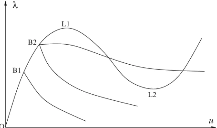
4 Stability analysis
when the equilibrium path reaches a local extremum, as the points L1 (maximum) and L2 (minimum), while a bifurca-tion occurs when different equilibrium paths cross at a certain point, as the points B1 and B2 in Fig. 2. Moreover, bifurca-tion points can be simple (as B1) or multiple (as B2). In this work, only simple critical points are discussed.
It is important to note that the stability theory discussed here is restricted to the case of symmetric stiffness matrices, since displacement dependent loads were not considered in the present work. On the other hand, the consideration of these loads leads to an unsymmetric stiffness matrix which requires a more complex treatment [27–29].
A point (u,λ) of the load-displacement curve is a critical point when the stiffness matrix of the FE model is singular. Thus, a critical point can be detected using the condition
detK(u, λ)=0. (57)
An alternative approach to the critical point detection is to use the zero eigenvalue condition
K(u, λ)φ=0, with φ =1, (58) whereφ is the associated eigenvector which represents the buckling mode of the structure.
4.1 Classification of simple stability points
Once detected a critical point, it is necessary to determine whether it is a limit or a bifurcation point. To perform this task, it is convenient to describe the load-displacement curve using a single parameter (s) that never decreases during the loading process, like the total arc-length. Using the paramet-ric form, the equilibrium equation can be written as
r(u(s), λ(s))=0, (59)
and its differentiation w.r.t. the curve parameter yields
˙
r=r,uu˙+r,λλ˙ =Ku˙+r,λλ˙ =0, (60)
where(·)indicates differentiation with respect tos.
Considering the symmetry of the stiffness matrix and us-ing the condition (58), it can be shown thatφtK = 0at a
O
L1
B2
B1
L2
u
λ
Fig. 2 Limit and bifurcation points
critical point. Therefore, the multiplication of the Eq. (60) by
φtleads to
(φtf)λ˙ =0, (61)
where the relationf = −r,λ defined by Equation (28) was used again. As pointed out earlier, a limit point is charac-terized by the fact that the load-displacement curve reaches an extremum value, so the condition λ˙ =0 must hold for these points. Therefore, the following criterion can be used to classify the critical points:
φtf=0⇒limit point
φtf=0⇒bifurcation point (62)
From a computational point of view, it is not convenient to use the expression (62) since the scalar productφtf at a bifurcation point generally does not vanish completely due to numerical errors. Thus, a slightly modified criterion will be used in this work:
φtf
φ f
> t ol⇒limit point
≤t ol⇒bifurcation point, (63)
andt olis a tolerance in the range between 10−3 and 10−7. Geometrically, the r.h.s of Eq. (63) represents the cosine of angle between vectorsφandf. It is important to note that the criterion adopted in the present work is not affected by the number of degrees of freedom of the FE model. Obviously, care should be taken whenfis close to zero. Bifurcation points of structures subjected only to mechanical loads are characterized by the orthogonality between the external load vector and the buckling mode [30, 31, 5]. However, for struc-tures subjected to thermal loading this is not a valid criteria since it is necessary to include the vectorg,λwhich, according to Eq. (13), is not a part of the external load vector.
In order to classify the bifurcation types it is necessary to use higher-order terms. The differentiation of Eq. (60) yields
Ku¨+r,λλ¨ = −(K,uu˙u˙ +2K,λu˙λ˙ +r,λλλ˙2). (64)
Moreover, the tangent to the equilibrium path at a bifur-cation point [32] can be written as
˙
u=ξ0u+ξ1φ ˙
λ=ξ0,
(65)
with
Ku+r,λ =0, ||u|| =1 and φtu=0. (66)
It can be noted that the vectorudefined above is closely related to the vectorδudefined by Eqs. (28) and (30), which corresponds to the predictor direction of the constrained New-ton-Raphson methods discussed in Sect. 3.2. At a bifurcation point, the multiplication of Eq. (64) byφtleads to
φt(K,uu˙u˙+2K,λu˙λ˙+r,λλλ˙2)=0, (67) which after the substitution of (65) yields the algebraic bifur-cation equation
where
a=φtK,uφ φ
b=φt(K,uu+K,λ)φ
c=φt(K,uu u+2K,λu+r,λλ).
(69)
In order to solve Eq. (68) it is necessary to constrain the size of the tangent vector. The use of the spherical arc-length constraint
˙
||u||2+ ˙λ2=1 (70)
yields the normalization condition
2ξ02+ξ12=1. (71)
The quadratic Eq. (68), together with the normalization condition, provides two sets of solutions ξ0 andξ1, corre-sponding to the two tangents at a simple bifurcation point, one tangent to the primary path and other tangent to the sec-ondary (bifurcated) path. The tangent to the primary path is associated with the vectoru˙closer to the predictor direction
δuof the path-following method used to trace the primary equilibrium path before the critical point. The other solution, tangent to the secondary path, can be used in the branch-switching procedure.
Defining the scalard =b2−ac, the simple bifurcation points can be classified [28] as
a=0 andb=0⇒pitchfork bifurcation
a=0 andd >0⇒transcritical bifurcation
d <0 ⇒isola formation point
d=0 ⇒cusp point.
(72)
The case of symmetric (or pitchfork) bifurcation is par-ticularly important to structural mechanics. Since in this case
a=0, the solution associated with the secondary path is given byξ0=0 andξ1 =1. Therefore
˙
u=φ and λ˙ =0. (73)
This equation is the theoretical basis of the eigenmode injection techniques used for branch-switching [30].
The derivativeK,u is not generally available in a finite element program. However, approximate derivatives based on the expression
K,uu1u2=lim
ǫ→0
K(u+ǫu1, λ)u2−K(u, λ)u2
ǫ (74)
can be used [27]. For mechanical loading without displace-ment dependent loads, the derivativesK,λandr,λλvanish and
need not to be computed. This is not the case of thermally loaded structures whereKandrdepend onλ. In the common case of linear elastic materials with temperature independent properties, bothKandgare linear functions ofλand the use of simple forward finite differences yields exact results (up to small round-off errors) regardless of the perturbation size.
4.2 Computation of critical points
The computation of critical points can be performed using the equilibrium Eqs. (13) and constraints enforcing the critical condition through the use of Eqs. (57) or (58). The resulting systems of nonlinear equations (extended systems) are gen-erally solved using a Newton-Raphson technique. Different extended systems were proposed for evaluation of critical points of FE models [33, 30, 29, 34]. Other approaches based on bisection or interpolation along the equilibrium path can also be applied [31].
In this work, the extended system based in the use of Eqn. (58) will be applied [33]. Thus, the system to be solved is given by
r(u, λ) K(u, λ)φ
φ −1
=0, (75)
where the eigenvector length constraint is necessary to avoid the trivial solution (φ = 0). The solution of this extended system gives the critical point (u,λ) as well as the buckling mode (φ), which can be used for the critical point classifi-cation. Since only one eigenvector is included in the system, this procedure is restricted to simple critical points [33].
The linearization of the expression (75) yields the system
K 0 r,λ
(Kφ),u K (Kφ),λ 0t φ
t
φ 0
δu δφ
δλ
= −
r Kφ
φ −1
, (76)
where
(Kφ),uδu=lim
ǫ→0
K(u+ǫ δu, λ)φ−K(u, λ)φ
ǫ
(Kφ),λδλ=lim ǫ→0
K(u, λ+ǫ δλ)φ−K(u, λ)φ
ǫ
(77)
are the directional derivatives of the stiffness matrix with re-spect to the displacement and load factor, rere-spectively. Eq. (76) allows the computation of the incrementsδu,δφandδλ. This system has 2N +1 variables and equations, but it can be solved in a simple and efficient way [33], as shown in Table 1.
After the computation of the increments, the variables (u,
λ,φ) are updated as indicated in Eq. (32), while the current eigenvalue (µ) can be computed from
µ=φtKφ. (78)
The procedure stops when both the residual and the eigen-value are smaller than prescribed tolerances.
Table 1 Solution of the extended system 1.Solve the systems:
Kδu1=f Kδu2=r
2.Compute the directional derivatives: h1=(Kφ),uδu1+(Kφ),λ
h2=(Kφ),uδu2 3.Solve the systems:
Kδφ1=h1 Kδφ2=h2
4.Compute the increments:
δλ=φ
t
δφ2− φ
φtδφ1
δu=δλ δu1−δu2
δφ=δφ2−δλ δφ1−φ
The success in the computation of critical points using extended systems depends on the evaluation of vectors h1 andh2. These vectors depend on the derivatives(Kφ),uand
(Kφ),λ. Starting from the expression of the strain energy, it is
possible to find the analytical expressions of the directional derivatives [33]. However, the practical application of the analytical approach is limited to simple elements, and to find a more general solution, it is interesting to use an approximate method.
The finite difference method can be used to computeh1 andh2in a simple and efficient way [30]. Using the forward difference scheme, these vectors can be computed from
h1=[K(u+ǫφ, λ) δu1−K(u, λ) δu1]/ǫ+hλ
h2=[K(u+ǫφ, λ) δu2−K(u, λ) δu2]/ǫ
hλ=[K(u, λ+λ)φ−K(u, λ)φ]/λ,
(79)
whereλis the same perturbation used in Eq. (40). Finally, by using definitions of Step (1) of Table 1
h1=[K(u+ǫφ, λ) δu1−f]/ǫ+hλ h2=[K(u+ǫφ, λ) δu2−r]/ǫ.
(80)
Since they do not depend on the element type, the expres-sions above can be implemented once and used for all avail-able element types of a given FE program. Generally, a per-turbation (ǫ) in the range
10−8< ǫφ/u<10−3, (81)
leads to accurate results [17]. The influence of the perturba-tion size in the convergence of the critical point computaperturba-tion was studied in this work by using a set of numerical exam-ples and the results will be presented in Sect. 5. Finally, it is important to note that the computation of the global vectors
h1andh2is carried out summing up the contribution of each element, using exactly the same procedure applied for the assembly of the global internal force vector.
For problems with only displacement independent mecha-nical loads (e.g. dead load),f =f and(Kφ),λ = 0. Before
this work, this was the only case considered in practical appli-cations of the extended systems to the computation of stabil-ity points of structures using the Finite Element Method [33,
30, 17, 24, 29, 34]. However, the simple modifications indi-cated here are sufficient to deal with thermal loads. As stated earlier, the derivativesg,λand(Kφ),λcomputed by forward
finite differences are exact (up to small round-off errors) for structures made of linear elastic materials and temper-ature independent properties. For other cases, these numer-ical derivatives are only approximations, but have sufficient accuracy to achieve convergence provided that the appro-priate perturbation is applied. The computation of critical points of thermally loaded structures is slightly more costly than computation for mechanically loaded structures, since it requires the computation of(Kφ),λ, which is not necessary
for the latter case.
Theoretically, the extended system described by Eq. (75) can be used to directly compute the critical point of a structure without tracing the equilibrium path before this point. How-ever, this is hardly the case in practical applications since the numerical algorithm may diverge if started far from the criti-cal point. Moreover, for structures with several criticriti-cal points there is no guarantee for which point the algorithm will con-verge. Actually, different solutions can be found depending on the initial valuesu0,λ0, andφ0.
Therefore, it is recommended to trace the equilibrium path using some of the algorithms described in Sect. 3 until a stability point is passed, which can be easily detected by the change in the number of negative pivots ofKafter the
LDLtfactorization, and then start the critical point computa-tion. This procedure guarantees a good starting point (u0,λ0) for the use in the extended system. For the initial eigenvec-tor (φ0) it is recommended to use an estimate of the current eigenvector ofKwhen a bifurcation point is expected or to use φ0 = u0/u0when a limit point is more likely [33]. As discussed in Sect. 3.2.2, the sign of the predictor work increment (ftδu) changes when a limit point is passed, so this criterion is used here to decide if a limit or bifurcation point is expected. Finally, an approximation of the smallest eigenvector ofKcan be computed in an inexpensive way by using the inverse iteration scheme.
The strategy of using a path-following method to get close to a critical point together with using the presented extended system to accurately compute this point worked very well in the numerical examples presented in Sect. 5. An alternative approach to avoid the convergence problems of the extended system approach to directly compute a critical point without tracing the equilibrium path is the homotopy method [35]. This approach is not addressed in this work.
4.3 Branch-switching
f =(utφ)2−l2 =0. (82) This constraint ensures that the size of the projection of the incremental displacement vector (u) along the buck-ling mode (φ) is l. According to Eq. (31), the consistent linearization yields
δλ= −(u
tφ)φtδ
ˆ
u+0.5f
(utφ)φtδu . (83)
Considering thatf is generally close to zero and can be neglected, then
δλ= −φ
tδuˆ
φtδu. (84)
Geometrically this means that δu is orthogonal to φ. Therefore, this procedure is most unlikely to return to the primary path, as it was verified in the numerical examples presented in Sect. 5. Instead of (84), the quadratic Eq. (48) with appropriate coefficients replacing (49) can also be used [24]. However, the use of this quadratic equation is more complex and was not adopted here.
Finally, based on Eq. (73), the predictor can be taken as
λp=0 and up=ηφ. (85)
According to Eq. (82),η = ±l. However, for perfect structures,l in the pre-buckling steps depends essentially on the load terms, while in post-buckling steps it depends essentially on the displacement terms. Therefore, it is not adequate to use the same arc-length in both situations and it is necessary that the user chooses theηvalue. As a guide-line this value should not be so small to avoid returning to the primary path and not so large to avoid convergence problems [31].
The other technique successfully used here consists in the application of the displacement control method described earlier, but choosing the controlling dof (k) as the maximum component of the buckling modeφand using the predictor
λp=0 and up= η φk
φ. (86)
As a consequence of this predictor,uk =η. For
sym-metric bifurcations,φ is orthogonal to the primary path, so this procedure is not likely to return to the primary path.
It is important to note that the procedures discussed in this section should be used only in the first step of the second-ary path and that the conventional Cylindrical Arc-Length Method (Sect. 3.2.2) should be used in the next steps. How-ever, at the end of the first step on the secondary path, the arc-length should be computed as
l =ut
sus, (87)
whereusis the displacement increment in the first step on
the secondary path. In the next stepsl should be updated according to Eq. (56). The procedures discussed here are restricted to simple bifurcation points, since only one eigen-vector is considered.
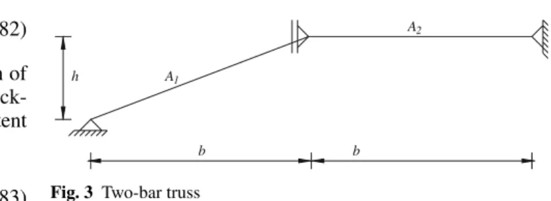
b b
h A
A
1
2
Fig. 3 Two-bar truss
5 Numerical examples
In this section a set of numerical examples will be used to validate the techniques presented in this work to the nonlin-ear analysis of structures subjected to thermal loading. The examples are concerned with the post-buckling behavior of different types of structures. In each example, the tolerances used to check the convergence of the path-following method and of the critical point computation are identical.
In order to assess the influence of the perturbation size used in the finite difference computation of the directional derivatives, the critical point computation in some examples will be performed using different perturbations. To eliminate the influence of the length of the nodal displacement vector (u), the perturbation size (ǫ) is computed from
ǫ=ǫ max(1,u/φ), (88)
whereǫis the prescribed relative perturbation. The critical points were computed here usingǫfrom 10−3to 10−7.
5.1 Two-bar truss
The first example is the two-bar truss depicted in Fig. 3. This simple truss has only one dof, which is the vertical displace-ment (v) of the central node. Here the nonlinear behavior due to temperature increase only in the horizontal bar is studied. The numerical properties used here are: b = 1.0 m,h = 0.25 m, A2/A1 =5, E = 70 GPa, andα =23×10−6 oC, whereAis the area of cross section.
Considering temperature independent properties, it can be easily shown that
Tcr =
1
α EA1
EA2
L2h2
L31 . (89)
For the numerical data used here Tcr = 496.24oC.
The temperature-displacement curve computed using total Lagrangian elements and the Arc-Length Method (t ol = 10−6andId =2) is shown in Fig. 4. It should be noted that
for this simple structure, the numerically computed bifurca-tion temperature is identical to the analytical one. After the critical point computation the branch-switching (η= ±0.01) is performed and the secondary paths are traced.
-0.12 -0.06 0 0.06 0.12 v/b
0 0.5 1 1.5 2
∆
T/
∆
Tcr
imp = 1/100 perfect
imp = -1/100
Fig. 4 Two-bar truss - equilibrium paths
Fig. 5 Slender rod - geometry and buckling mode
the safe temperature increase of this truss is given by the limit point (T /Tcr =0.8263), since there are no
unsta-ble points at smaller temperatures. Forǫ=10−3the critical point computation required 7 iterations, while for the other perturbations only 5 iterations were necessary.
In order to assess the imperfection sensitivity of this truss, geometric imperfections withh/ h = ±1/100 were also considered here. It can be concluded that the introduction of the imperfection eliminates the bifurcation (unfolding) and further decreases the load-carrying of the structure in the unstable branch. Moreover, the curves of the imperfect structures are similar to the perfect ones, with the difference decreasing as displacements increase.
5.2 Slender rod
This example deals with a slender elastic rod with hinged supports. It is closely related to the Euler column, but the hor-izontal displacement is restrained in both supports in order to generate compressive forces. Figure 5 shows the geome-try and boundary conditions of the rod as well as the buck-ling mode computed here by finite element analysis. The fol-lowing properties were used in the numerical computations:
L=5.0 m,A=10−3m2,I =2.5×10⁻⁶m4,E=200 GPa, andα=12×10−6 oC, whereLis the rod length andI the moment of inertia.
The buckling temperature of this rod can be easily com-puted equating the compressive force generated by the tem-perature increase (EAαTcr) with its buckling load
(π2EI /L2). Therefore
Tcr= π2
α(L/r)2, (90)
wherer =√I /Ais the radius of gyration of the cross sec-tion. This equation shows that the buckling temperature does not depend on the Young’s modulus, but only on the thermal expansion coefficient and on the slenderness ratio (L/r). For the numerical data used hereTcr =82.247oC.
The rod was discretized using 10 corotational plane frame elements with higher-order terms in axial strain computation [4]. The perfect column was analyzed using the Arc-Length Method (t ol=10−6andId =3). The critical point
computa-tion and the branch-switching (η= ±0.01) were easily per-formed. As a matter of fact, the computation of the bifurcation temperature required only 3 iterations for all relative pertur-bations (ǫ) used here. The computed critical temperature was
Tcr=82.248oC, which is in very good agreement with the
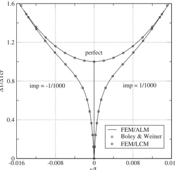
analytical one. The curves of temperature versus transversal displacement of the central node (v) are presented in Fig. 6. These curves clearly show a stable-symmetric bifurcation.
The finite element curves are in very good agreement with the approximate post-buckling response
v L=2
r L
T Tcr −
1 (91)
given by Boley & Weiner [36]. It is interesting to note that the post-buckling resistance of a rod subjected to thermal load-ing is not negligible, sinceT /Tcr = 1.250 forv/L =
1/100. This behavior is completely different from the classi-cal case of mechaniclassi-cal loading, whose elastica solution yields
P /Pcr=1.015 forv/L=11/100 [37], wherePis the
com-pressive force.
-0.016 -0.008 0 0.008 0.016 v/L
0 0.4 0.8 1.2 1.6
∆
T/
∆
Tcr
FEM/ALM Boley & Weiner FEM/LCM perfect
imp = 1/1000 imp = -1/1000
1 1.5 2 2.5 3 ∆T/∆Tcr
0.999 0.9992 0.9994 0.9996 0.9998 1
P/Pcr
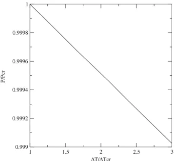
Fig. 7 Slender rod - compressive force
The imperfection sensitivity is investigated here using an imperfection with the shape of the numerically computed buckling mode. It can be noted that even for the very small imperfection ymax/L = ±1/1000 presented in this figure,
there is a significant difference between the perfect and imper-fect cases in the pre-buckling range. However, the two results are almost identical for large displacements. The imperfect columns were analyzed using both the Arc-Length Method (ALM) and the Load Control Method (LCM) leading to iden-tical results, indicating that the implementation of both meth-ods is correct.
Finally, Fig. 7 shows the variation of the compressive force with the temperature increase in the post-buckling range. It can be noted that the compressive force remains practically constant after buckling, as assumed in the development of Eq. (91). Moreover, this slight decrease in the compressive force was also reported in the analytical solution based on elliptic integrals [38], confirming that an early solution pre-dicting the increase of the compressive force was incorrect [38].
5.3 Heated pipeline
Oil pipelines under thermal and internal pressure loading de-velop significant compressive forces due to the axial expan-sion restraint provided by the soil. Such forces may induce lateral (snaking) and vertical (upheaval) buckling. The lateral buckling temperature is smaller than the vertical one unless the pipeline is buried [39]. However, subsea pipelines gener-ally should be buried to protect them from damage by anchors and trawling gear, making the upheaval buckling the primary concern in design of such pipelines [40].
An important problem in practical applications is the anal-ysis of pipelines with prop imperfections, as depicted in
Fig-ure 8. The prop may actually be an undercrossing non-parallel pipe or an intervening rock. Using simple statics, it can be shown [40] that the imperfection shapey(x)is given by
y= q
72EI
2Lp
Lp
2 −x
3 −3
Lp
2 −x
4
, (92)
whereqis the self-weight,x is the distance from the prop center, andLpis the imperfection length. As a consequence,
Lp=
1152EI yp q
1/4
. (93)
The pipe was modeled by corotational plane frame ele-ments, while the soil was modeled by isoparametric (2 noded) elements based on Winkler theory. These soil elements allow different nonlinear reaction-displacement curves in axial and vertical directions. In order to simplify the analysis and allow the comparison with some analytical results, almost rigid-plastic behavior is assumed here both in axial and vertical directions. Thus, a very small yielding displacement (1 mm) is used in the elasto-plastic soil curve in both directions.
The reaction-displacement curve in axial direction is sym-metric about the origin with an ultimate resistance that can be related with the pipe weight using a friction coefficient (µ). On the other hand, to simulate the unilateral contact condition between the pipe and a rigid base, considered in the analytical procedures [39], the reaction-displacement curve in vertical direction should be asymmetric, with the ultimate resistance in upward direction given by the pipe weight (including the soil cover) and with a large stiffness in the downward direc-tion to prevent the penetradirec-tion in the soil. Here, the ratio be-tween upward and downward stiffnesses is taken as 1/1000. The pipe and soil properties considered in this example areD=0.65 m,t =0.015 m,q=3.8 kN/m,E=200 GPa,
α=11×10−6 oC, andµ=0.5. It can be shown that the post-buckled configuration of a pipeline is composed by a buck-led region and an adjoining region [39]. The buckbuck-led region presents large vertical displacements, while the adjoining re-gion presents only axial displacements. Using the analytical procedure for perfect pipelines [39], the safe temperature in-crease, the buckling length and the length of the adjoining region are 62.459oC, 96.4 m and 736.3 m, respectively.
Considering the symmetry conditions, only half of the pipeline needs to be discretized. Using the analytical results as a guideline and considering that the buckled region re-quires a finer mesh than the adjoining region, the mesh used here was divided in three regions, the first one with 100 m and 200 elements (buckled region), the second one with 1000 m and 200 elements (adjoining region) and the third region with 2000 m and 10 elements to model the portion of the pipe-line far away from the buckled region where the compressive
Prop y
L p
p
0 3 6 9 12 v (m)
0 40 80 120 160
∆
T (
°
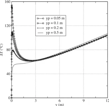
C)
yp = 0.05 m yp = 0.1 m yp = 0.2 m yp = 0.5 m
Fig. 9 Heated pipeline – equilibrium paths
forces are constant. The same discretization was used for the soil elements. The axial displacement is constrained at both initial and final nodes, resulting in a model with 1210 dofs.
The equilibrium paths for different prop heights deter-mined by using the Cylindrical Arc-Length Method (t ol = 10−4 and Id = 3) are presented in Fig. 9. The curves for
small props show that the pipeline presents two limit points, a maximum and a minimum. Therefore, the curves present an initial stable state (pre-buckled), followed by an unsta-ble state (post-buckled) and a final staunsta-ble state at large dis-placements. Since there are not unstable equilibrium points at temperatures smaller than the temperature of the second limit point, this temperature is generally called the safe tem-perature increase (Tsaf e) of the pipeline.
The smaller limit point for each prop height was com-puted by the algorithm described in Sect. 4. Foryp=0.05 m,
the safe temperature increase computed here was 61.722oC with a buckling length of 95.0 m, which is fairly close to the analytical values obtained for perfect pipelines. The algo-rithm for critical point computation converges quickly for this problem, requiring only 3 iterations for all relative per-turbations (ǫ) used here. The curves show that the increase of prop height brings the limit points close to each other, until they coincide and finally disappear. As a matter of fact, the curves corresponding to large prop heights do not have any limit points presenting a stable behavior.
The pipe with a prop imperfection of 0.2 m was also ana-lyzed considering two different weights to study the effect of an increase in the soil cover. The results presented in Fig. 10 show that the two curves are almost parallel and that there is an increase in the pipeline safe temperature. In fact,Tsaf e
increases from 61.010oC to 68.845oC (12.8%) whenq in-creases from 3.8 kN/m to 4.75 kN/m (25%). These curves also show that the Arc-Length and Displacement Control
methods successfully traced the complete equilibrium paths, generating coincident curves.
On the other hand, the curves obtained by using the Load Control Method (T =1oC) clearly show the snap-through phenomenon, with the equilibrium path missing the limit point corresponding to the safe temperature increase. Another problem of this method was the large number of iterations (≈ 100) required in the step corresponding to the snap-through. However, since the results of the three methods are consistent, it can be concluded that the numerical differ-entiation approach used to compute g,λ required by both
Arc-Length and Displacement Control, can be used with con-fidence for practical finite element analysis.
5.4 Cylindrical shell
The cylindrical shell depicted in Fig. 11 has been studied by a number of authors for mechanical [41, 15] and thermal loading [7, 8]. This shell was analyzed here for different rela-tionsa/ h, wherehis the shell thickness. The numerical data used here are R = 2540 mm,a = 508 mm,γ = 0.2 rad,
E=3105 N/mm2, andα=20×10−6 oC. The shell bound-aries are simply supported.
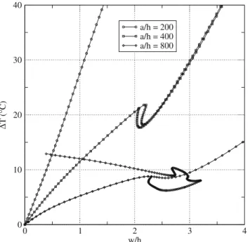
The shell was analyzed using a mesh of 10×10 quadratic (8 noded) finite elements, resulting in 1541 dofs. Theses ele-ments are based on the Marguerre’s theory for shallow shells and formulated according to the total Lagrangian approach [42]. The equilibrium paths computed by the Arc-Length Method are presented in Fig. 12, where w is the transver-sal displacement of the central node.
These paths show that the nonlinear effects sharply in-crease with thea/ hratio. Fora/ h= 400 anda/ h=800 the paths present limit point, snap-backs, and bifurcations
0 2 4 6 8 10 v (m)
30 45 60 75 90 105
∆
T (
°
C)
Arc-length
Displacement control Load control
q = 4.75 kN/m
q = 3.8 kN/m
R
a
γ γ
Fig. 11 Shallow shell
(simple and multiple). Thus, the figure shows the primary and secondary paths. It should be noted that only the first secondary path of each example is depicted in this figure, but other bifurcation points were located along both primary and secondary paths.
This example clearly shows the importance of computing the critical points and tracing the secondary paths even when the primary path is already nonlinear. As a matter of fact, the curve for a/ h = 400 presents a bifurcation point, which the conventional path-following without branch-switching would miss, that is smaller than the first limit point. Finally, it can be noted that the procedures discussed in this paper are robust enough to handle this complex problem with a significant number of dofs.
0 1 2 3 4
w/h 0
10 20 30 40
∆
T (
°
C)
a/h = 200 a/h = 400 a/h = 800
Fig. 12 Shallow shell – equilibrium paths
6 Concluding remarks
This work addressed methods to trace the equilibrium paths of structures subjected to thermal loading, including the critical point computation and the branch-switching to the secondary paths at bifurcation points. In spite of its importance to engi-neering practice, this subject has not been properly discussed in the literature.
Using the concept of effective strains and performing the consistent linearization of the governing nonlinear equations, the expressions required to implement the different path-fol-lowing methods were fully developed here for problems with geometric and material nonlinearity. It was shown that the Load Control Method already implemented for mechanical loads can be used for thermal loads without modification. The same occurs with the computation of the internal force vector and the tangent stiffness matrix.
On the other hand, the case of Constrained Newton-Raph-son Methods is more complex since the linearization of the residual vector leads to the necessity to compute the deriv-ative of the internal forces with respect to the load factor, which is not required for pure mechanical loading. The ana-lytical expression of this vector was presented, but numerical differentiation was successfully used in different examples and is recommended for practical implementation. The pit-falls presented by the Displacement Control Method and by the Cylindrical Arc-Length Method to structures whose pre-buckling displacements are null were discussed and the use of the Spherical Arc-Length was recommended as a practical solution to this problem. On the other hand, the use of the cylindrical version is recommended to trace the secondary paths since it is more simple (ψ =0) and efficient than the spherical version [15, 16, 23].
The classification and computation of critical points using extended systems were also thoroughly discussed. The main difference from the case of mechanical loads is the need to compute the derivative of the internal force vector and of the stiffness matrix with respect to the load factor. The numer-ical differentiation approach was successfully applied here and it was verified that the standard forward finite differ-ence scheme yields exact results for the important case of linear elastic materials with temperature independent prop-erties. Two branch-switching techniques were discussed and successfully implemented.