A New Method for Static Video
Summarization Using Visual Words
and Video Temporal Segmentation
Edward Jorge Yuri Cayllahua Cahuina
Federal University of Ouro Preto
Catalogação: [email protected]
C132 Cahuina, Edward Jorge Yuri Cayllahua.
A new method for static video summarization using visual words and video temporal segmentati [manuscrito] / Edward Jorge Yuri Cayllahua Cahuina – 2013.
88f.: il.; grafs.; tabs.
Orientador: Prof. Guillermo Cámara Chávez.
Dissertação (Mestrado) - Universidade Federal de Ouro Preto. Instituto de Ciências Exatas e Biológicas. Departamento de Computação. Programa de Pós-graduação em Ciência da Computação.
Área de concentração:Recuperação e Tratamento da Informação.
1. Vídeo – Teses. 2. Estrutura de Dados (Computação) - Teses. 3. Descritores - Teses. 4. Sistemas de recuperação da informação - Teses. I. Cámara Chávez, Guillermo. II.
Universidade Federal de Ouro Preto. III. Título.
iii
A New Method for Static Video
Summarization Using Visual Words and
Video Temporal Segmentation
Abstract
During the last years, a continuous demand and creation of digital video information have occurred. The creation of digital video has caused an exponential growth of digital video content. To increase the usability of such large volume of videos, a lot of research has been made. Video summarization, in particular, has been proposed to rapidly browse large video collections. It has also been used to efficiently index and access video content. To summarize any type of video, researchers have relied on visual features contained in frames. In order to extract these features, different techniques have used local or global descriptors. Nonetheless, no extensive evaluation have been made about the usefulness of both types of descriptors in video summarization.
iv
Durante os ´ultimos anos, uma demanda cont´ınua de informa¸c˜oes de v´ıdeo digital ter ocorrido. A cria¸c˜ao de v´ıdeo digital tem provocado um crescimento exponencial de conte´udo de v´ıdeo digital. Para aumentar a usabilidade de grande volume de v´ıdeos, muita pesquisa tem sido feita. A Sumariza¸c˜ao Autom´atica de V´ıdeos , em particular, tem sido proposto para explorar rapidamente grandes colec¸c˜oes de v´ıdeo. Os resumos de videos tem sido utilizado de forma eficiente para indexar e conte´udos de v´ıdeo de acesso. Para resumir qualquer tipo de v´ıdeo, os pesquisadores tem usado as caracter´ısticas visuais contidas nos quadros do video. A fim de extrair essas caracter´ısticas, diferentes t´ecnicas tˆem utilizado descritores locais ou globais. No entanto, nenhuma avalia¸c˜ao extensa tˆem sido feita sobre a utilidade de ambos tipos de descritores na sumariza¸c˜ao autom´atica de v´ıdeos.
v
Acknowledgements
First and above all, I praise God, for providing me this opportunity and granting me the capability to proceed successfully. This dissertation appears in its current form due to the support and guidance of several people. I would therefore like to offer my sincere thanks to all of them.
I would like to express my gratitude to my advisor and friend, Professor Guillermo Camara Chavez, whose guidance and patience has been of great help and made possible this dissertation to finish.
I would not have contemplated this road if not for my parents, Jorge and Benilda. To my parents, thank you for your continuous support which encouraged me to study abroad.
To my dear friend, Rensso Mora Colque, whose friendship made my stay at Brazil a good experience.
Conte´
udo
Lista de Figuras xi
Lista de Tabelas 1
1 Introduction 3
1.1 Introduction . . . 3
1.2 Motivation . . . 7
1.3 Aims and Objectives . . . 7
1.3.1 General Objective . . . 7
1.3.2 Specific objectives . . . 8
1.4 Contributions . . . 8
1.5 Thesis Outline . . . 9
2 State of Art 11 2.1 Introduction . . . 11
2.2 Methods Based on Image Descriptors . . . 12
2.3 Methods Based on Mid-level Semantics . . . 14
2.4 Methods Based on Text (Video Annotation) . . . 15
2.5 Methods Based on Audio . . . 16
2.6 Final Considerations . . . 17
3 Theoretical Fundamentals 19 3.1 Digital Video . . . 19
3.1.1 Terminology . . . 20
3.2 Visual Effects in Videos . . . 21
3.2.1 Cut . . . 21
3.2.2 Fades and Dissolves . . . 22
3.3 Image Descriptors . . . 23
3.3.1 Color Histogram . . . 23
viii Conte´udo
3.3.2 Projection Histograms . . . 25
3.3.3 Scale-Invariant Feature Transform (SIFT) . . . 25
3.3.4 A SIFT Descriptor with Color Invariant Characteristics (CSIFT) 30 3.3.5 HUESIFT . . . 31
3.3.6 SURF: Speeded-Up Robust Features . . . 31
3.3.7 Space-Time Interest Points (STIP) . . . 32
3.3.8 Histograms of Oriented Gradients (HoG) . . . 35
3.4 Classification . . . 37
3.4.1 K-means . . . 37
3.4.2 X-means: Extending K-means with Efficient Estimation of the Number of Clusters . . . 38
3.5 The Bag-of-Words model . . . 40
3.6 Final considerations . . . 40
4 Proposed Method 43 4.1 Proposed Method for Summarizing Videos . . . 43
4.1.1 Temporal Video Segmentation . . . 44
4.1.2 Detection of Representative Frames . . . 46
4.1.3 Bag of Words (BoW) . . . 47
4.1.4 Histogram of Visual Words . . . 48
4.1.5 Visual Word Vectors Clustering . . . 48
4.1.6 Filter Results . . . 49
4.2 Final Considerations . . . 49
5 Experimental Results 53 5.1 Data Set . . . 53
5.2 Experimental setup . . . 56
5.3 Video Summary Evaluation . . . 57
5.4 Experiments . . . 59
5.4.1 Results for the Open Video Database . . . 59
5.4.2 Results for the Youtube Database . . . 61
5.5 Final Results Analysis . . . 62
5.6 Final Considerations . . . 63
Conte´udo ix
Lista de Figuras
1.1 A general approach for video summarization . . . 4
1.2 Illustration of a video sequence with shots and transitions. Shots are S1, S2, S3 and S4, TP is the transition period. . . 6
3.1 Anatomy of a video . . . 20
3.2 A fade-in transition . . . 22
3.3 A fade-out transition . . . 23
3.4 A dissolve transition . . . 23
3.5 Difference of Gaussians . . . 27
3.6 Locating maxima/minima in DoG images . . . 28
3.7 The Bag-of-Words model . . . 41
4.1 Method for Summarizing Videos . . . 44
4.2 A dissimilarity vector computed from video HCIL Symposium 2002 -Introduction, segment 01 . . . 45
4.3 A refined dissimilarity vector computed from videoHCIL Symposium 2002 - Introduction, segment 01 . . . 50
4.4 Dissolve effect in videoHCIL Symposium 2002 - Introduction, segment 01 between frames 2139 - 2162 . . . 50
4.5 Variance vector for video HCIL Symposium 2002 - Introduction, segment 01. The circles are the detected dissolve effects . . . 51
xii LISTA DE FIGURAS
5.1 User Summary Number 1 for videoDrift Ice as a Geologic Agent, segment 08 . . . 63 5.2 User Summary Number 2 for videoDrift Ice as a Geologic Agent, segment
08 . . . 64 5.3 User Summary Number 3 for videoDrift Ice as a Geologic Agent, segment
08 . . . 64 5.4 User Summary Number 4 for videoDrift Ice as a Geologic Agent, segment
08 . . . 64 5.5 User Summary Number 5 for videoDrift Ice as a Geologic Agent, segment
08 . . . 65 5.6 Video Summary using the VSUMM1 approach for video Drift Ice as a
Geologic Agent, segment 08 . . . 65 5.7 Video Summary using SURF descriptor for videoDrift Ice as a Geologic
Lista de Tabelas
5.1 Videos used for experiments . . . 54 5.2 (Open Video Data Set) Experiments using temporal segmentation . . . . 60 5.3 (Open Video Data Set) Experiments without temporal segmentation . . . 61 5.4 (Youtube Data Set) Experiments using temporal segmentation . . . 62 5.5 (Youtube Data Set) Experiments without temporal segmentation . . . . 62
Cap´ıtulo 1
Introduction
1.1 Introduction
The amount of multimedia information such as text, audio, still images, animation, and video is growing every day. The accumulated volume of this information can become a large collection of data. A video is a perfect example of a multimedia resource that is in continuous generation. It would be an arduous work if a human tries to process such a large volume of data and even, at a certain scale, it would be impossible.
As a consequence of video information growth, an enormous quantity of video is uploaded to the Internet. TV video information is generated every day and security cameras generate hours of video. Furthermore, a video requires the user to watch the whole content to retrieve its information. This means that the user is forced to exclusively watch the video and is unable to do anything else during this time.
Due to this increased use of video and the human effort taken to process it, new technologies need to be researched in order to manage effectively and efficiently such a quantity of information. Video summarization has recently been of interest for many researchers due to its importance in several applications such as information browsing and retrieval (Xiong, Zhou, Tian, Rui and TS 2006, Valdes and Martinez 2011). A video summary is a short version of an entire video sequence and aims to give to a user a synthetic and useful visual abstract of a video sequence.
The final video summary must be a synopsis that can easily be interpreted by the user. This means that the summary must be presented in a user-friendly manner. The most important goal is to provide users with a concise video representation so that the user
4 Introduction
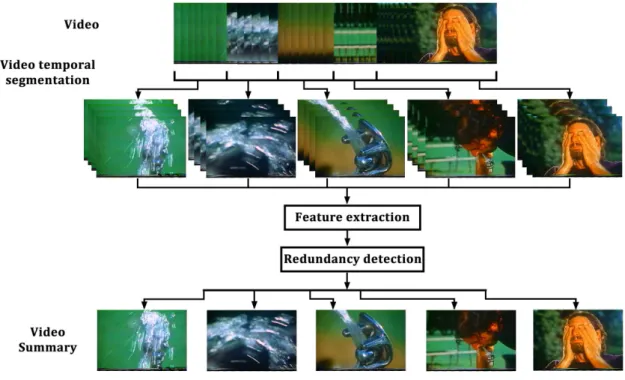
have a quick idea about the content of the video (Furini, Geraci, Montangero, Pellegrini, a1, a2 and a3 2010). This will help him/her decide whether to watch or not the whole video. Generally speaking, the task of video summarization has been approached by using different methods to cluster the video content and therefore, detect the redundancy of the video content in order to summarize it (Gao, Wang, Yong and Gu 2009). In Figure 1.1, a generic approach for video summarization is presented. The general steps involved are: a video segmentation, then a feature extraction process is performed, afterwards a redundancy detection based on the features is applied and finally the video summary is generated.
Figura 1.1: A general approach for video summarization
According to Truong and Venkatesh (2007) and Money and Agius (2008), the video summary can be represented into two fashions: a static video summary (storyboard) and a dynamic video skimming. Dynamic video skimming, also known as moving storyboard, consists in selecting the most relevant small dynamic portions (video skims) of audio and video in order to generate the video summary. The result is another video of shorter length. On the other hand, static video summary, or storyboard, is interested in selecting the most relevant frames (keyframes) of a video sequence and generate the correspondent video summary, which will be a collection of still images (Gao, Wang, Yong and Gu 2009).
Introduction 5
usually intended for final users; lately, this type of summary is in high demand (Xiang-Wei, Zhang, Zhao and Zhu 2009). Meanwhile, a static summary is more appropriate for indexing, browsing and retrieval. Furthermore, static video summaries have one important advantage, they allow the user to quickly have a general overview of the video content. On the other hand, in a dynamic video summary, the user is still required to watch a small version of the video in order to understand its content.
Both, static and dynamic video summaries can be computed independently of the genre of the video. However, some methods base their analysis on the type of video they are trying to summarize. For example, sports videos may be better summarized by the most important events like goals, fouls, etc., most of these events are based on motion information. Nevertheless, in a generic video, motion may not represent an important information because it may belong to a not relevant and isolated event.
In order to summarize a generic video, most of the methods (de Avila, ao Lopes, da Luz and de Albuquerque Ara´ujo 2011, Papadopoulos, Chatzichristofis and Papamarkos 2011, Yuan, Lu, Wu, Huang and Yu 2011) have heavily relied on visual features computed from video frames. Visual features can be used to describe the global or local characteristics of an image. Many methods have based their analysis on global or local image descriptors. However, there has not been a wide evaluation about the performance of these two types of descriptors applied to video summarization. In (Kogler, del Fabro, Lux, Schoeffmann and Boeszoermenyi 2009), an evaluation was performed but their data set was limited to only 4 small videos, and therefore it is not possible to achieve strong conclusions about the performance of local descriptors in video summarization.
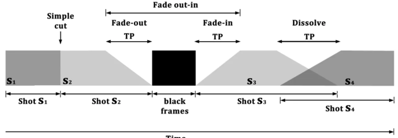
Another important consideration in video summarization is temporal video segmenta-tion. This task is usually performed by detecting transitions between shots and is often applied as the first step in video summarization. A shot is defined as an image sequence that presents continuous action which is captured from a single operation of a single camera. Shots are joined together in the editing stage of video production to form the final video, using different transitions. There are two different types of transitions that can occur between shots: abrupt (discontinuous) shot transitions, also referred as cuts; or gradual (continuous) shot transitions, which include video editing special effects (fade-in, fade-out, dissolving, etc). These transitions can be defined as:
6 Introduction
• fade-out: a shot gradually disappears from a constant image. • dissolve: the current shot fades out while the next shot fades in.
In Figure 1.2, a visual explanation of the different transitions can be seen.
Figura 1.2: Illustration of a video sequence with shots and transitions. Shots areS1, S2, S3
and S4, TP is the transition period.
A successful video temporal segmentation can lead into a better shot identification. Shots can be considered as the smallest indexing unit where no changes in scene con-tent can be perceived and higher level concepts are often constructed by combining and analyzing the inter and intra shot relationships (Camara Chavez, Precioso, Cord, Phillip Foliguet and de A. Araujo 2007). Therefore, we must outline the importance of an effective video temporal segmentation.
Introduction 7
1.2 Motivation
Researchers have acknowledged the importance of effectively and efficiently manage and browse large video collections. That is the reason why video summarization has been a popular topic of research during the last years. In order to provide meaningful and relevant video summaries, different methods have been proposed. Some methods propose a semantic analysis with the intention of producing more informative summaries. These methods have relied on object detection techniques in order to extract visual information to perform a semantic analysis. To do this, local descriptors have been widely used to describe the visual information contained in frames when summarizing videos. Despite its extensive use, there has not been an ample evaluation about the performance of local descriptors in video summarization.
This dissertation is mainly motivated by the necessity to realize an evaluation about the performance of global and local descriptors applied to video summarization using a large data set of over 100 videos. And also, to evaluate the importance of temporal video segmentation applied to video summarization. In order to elaborate a method that is capable of handling the video information and extract the most relevant frames contained in the video, a method for video summarization based on semantic information and temporal segmentation is proposed. Thus, providing the user a more informative previous knowledge about the video content.
1.3 Aims and Objectives
In this section, the main and specific objectives pursued in this dissertation are presented.
1.3.1 General Objective
8 Introduction
1.3.2 Specific objectives
1. Carry out a wide evaluation about the performance of local descriptors applied to video summarization.
2. Evaluate the importance of temporal video segmentation applied to video summari-zation.
3. Analyze the robustness of local descriptors compared to global descriptors.
4. Study the relevance of color information used by some local descriptors applied to video summarization.
5. Perform experiments using large datasets with all types of videos.
1.4 Contributions
During the last years, several approaches for video summarization have been proposed. Most of these approaches base their analysis on local or global visual features computed by descriptors. Nonetheless, there has not been an evaluation about what type of descriptor is better for video summarization. The main contribution of this dissertation is to present a method for static video summarization using semantic information and video temporal segmentation. We also perform a wide evaluation in order to achieve a stronger position about the performance of local descriptors in a semantic video summarization. Furthermore, we evaluate the robustness of local descriptors compared to global descriptors.
Additionally, another important thing to outline is that some local descriptors use color information and others do not. So far there has not been any evaluation on wether local descriptors using color information give more meaningful summaries compared to other local descriptors. Therefore, we also inspect if color information can help local descriptors to produce better video summaries.
Introduction 9
evaluate how local descriptors are affected by temporal segmentation and its importance in giving better video summaries.
Another important contribution of this dissertation is to propose a simple method for semantic video summarization that can produce meaningful and informative video summaries.
1.5 Thesis Outline
Cap´ıtulo 2
State of Art
Video summarization has been an active topic of investigation. Several methods have been created in order to synthesize large hours of video and overcome this problem. In this chapter, we present a review of different approaches that have been proposed for video summarization.
2.1 Introduction
The process of video summarization extracts the most relevant frames or segments of a video and produce a final sequence of images or portions of video. The final result should be easy to understand by the final user. Video summarization has been a popular topic of investigation and has attracted the attention of many researchers, making it a research topic that has been investigated for several years. Nonetheless, video summarization still poses a challenging problem. Video abstraction is still largely in the research phase (Truong and Venkatesh 2007).
Different approaches for video summarization have been developed so far. We can classify video summarization by the final presentation of the video summary. We have two types of methods: static and dynamic. Static methods produce the final summary based on selected keyframes. Therefore, the final result is a slideshow of these keyframes. The main advantage of this type of summary is that the user can access the information quickly, they can easily have a global review of the whole video content. The main disadvantage is that no audio, text or any other information is shown, just the most important frames of the video. On the other hand, dynamic methods select the portions of video that are considered to be relevant. Then, these portions are joined together.
12 State of Art
The result is a video that is smaller than the original and can contain audio information, it is a more comprehensible summary but the main disadvantage is that the user has to watch the whole summary video in order to understand the video content.
A different classification is proposed by Money and Agius (2008), they propose to classify video summarization methods in three categories: internal, external, and hybrid. The most popular approach for video summarization is the internal. It is called internal because the whole analysis is applied to the video stream only, so the methods only use the data that is self contained in the video. External methods use the information that is not necessarily contained in the video, such as manual annotation, labeling, etc. (Miyauchi, Babaguchi and Kitahashi 2003, Dagtas and Abdel-Mottaleb n.d.). The hybrid
methods use a combination of both internal and external information.
Internal methods have the main advantage that the whole method can be applied automatically using only the information contained in the video. Truong and Venkatesh (2007) present the different features used in the these approaches, the most popular features used are: visual, text, audio, visual dynamics, camera motion, mid-level semantics. Most of these features can only be applied to specific types of video. For example, we can easily extract visual, text and audio features in a movie or a sitcom, but all these features are not always present in the video captured by a cellphone or a security video.
In order to automatically summarize a video, an approach has to first extract the different features present in a video. Then, based on some similarity, it distinguishes which parts of the video can be considered as relevant and then extract these parts to build the summary. Therefore, the first step is to extract the features for posterior analysis. We will now present some of the existing methods in the literature. Since our work is more related to visual features, special attention to the methods that use visual features will be taken.
2.2 Methods Based on Image Descriptors
State of Art 13
Color histograms have often been used to measure the similarity between two frames, which is useful when the method’s goal is to summarize the video based on redundancy elimination. Zhuang, Rui, Huang and Mehrotra (1998) use a color histogram as the main descriptor. The idea is to segment the video in shots and form groups using an unsupervised clustering algorithm. Every frame will belong to a certain cluster based on its color histogram. Then, the closest frame to each centroid is marked as akeyframe and extracted to build the storyboard. Recent researches still use the simplicity and power of color histograms, such as the methods proposed by Furini, Geraci, Montangero, Pellegrini, a1, a2 and a3 (2010) and de Avila, ao Lopes, da Luz and de Albuquerque Ara´ujo (2011). They basically share the same general structure of histogram extraction and later perform an unsupervised clustering algorithm in order to produce the video summary.
Color histograms are usually vectors of high dimensionality. In order to overcome this problem, several methods have proposed to apply mathematical procedures on these feature vectors in order to reduce its dimensionality. Gong and Liu (2003) propose to use the singular value decomposition (SVD), later Mundur, Rao and Yesha (2006) and Wan and Qin (2010) use the principal component analysis (PCA). Also, in (Cahuina, Chavez and Menotti 2012), a static video summarization approach is presented using both color histograms and dimension reduction using PCA. Thus far, no comparisons have been performed between the two approaches. Furthermore, there has been no evaluation about the cost-benefit between the results obtained and the computational cost implied in performing these mathematical procedures.
14 State of Art
2.3 Methods Based on Mid-level Semantics
A more informative summary can be obtained if the method considers the semantic meaning implied in the video. Semantic comprehension is per se an active topic of research in computer vision and is still in progress, so far no method has perfectly performed semantic comprehension on images. Videos are composed by consecutive images, and these images can contain all types of objects. To delimitate the problem, some methods have based their analysis according to the interest of the final user and the input video that is going to be summarized. Miura, Hamada, Ide, Sakai and Tanaka (2003) try to summarize cooking videos performing a face detection procedure, the segments where faces are detected will not be considered in the final abstract since they have no cooking-related information. In contrast, (Peker, Otsuka, Divakaran, Peker, Otsuka and Divakaran 2006, Lee and Kim 2004, Peng, Chu, Chang, Chou, Huang, Chang and Hung 2011) perform face recognition in order to mark these segments as relevant ones, which is very important when summarizing movies, sitcoms or security videos. These methods are mainly interested in object recognition. In (zhiqiang Tian, Xue, Lan, li and Zheng 2011), a static video summarization based on object recognition is proposed. The idea is to eliminate redundancy of information from the temporal and spatial domain and also from the content domain by doing object recognition. The shot boundaries are detected and video objects are extracted using a 3D graph-based algorithm. Then, a K-means clustering algorithm is applied to detect the key objects.
In order to summarize sports videos, such as soccer, basketball, baseball, etc. The methods are more concerned about event detection. In (Fendri, Ben-Abdallah and Hamadou 2010), the method detects specific events (attacks, goals, etc.) and then produces a summary based on the event the user is more interested. Kim, Lee, Jung, Kim, Kim and Kim (2005) propose a method that not only performs event detection but also tracks the score. The goal is to give more importance to the previous moments before a ball goes into the basket, since they consider that finishing plays should be given more importance.
State of Art 15
In addition, for each shot they produce a histogram of occurrences of visual words using the visual word dictionary. Then, the histograms are grouped, meaning that similar visual entities will be grouped together. Finally, the video summary is produced by extracting the frames that contain the important visual entities. Papadopoulos, Chatzichristofis and Papamarkos (2011) also use the bag of visual words, but the object descriptor used is the SURF (Speeded Up Robust Features)(Bay, Ess, Tuytelaars and Van Gool 2008). Unfortunately, no evaluation has been performed between these descriptors applied to video summarization. Li (2012) analyzes the video content using the SIFT features to produce a static summary. The idea is to summarize the video based on the content complexity and the difference between frames. In order to do this, a video segmentation is applied based on the content complexity. Once the video is segmented, the detected shots are merged based on their similarity. Finally, the keyframes are extracted from the detected merged shots.
The SIFT descriptor has been widely used in computer vision for its ability to handle intensity, rotation, scale variations; this makes it a good descriptor but one disadvantage is its high computational cost.
Temporal information has also been used for video summarization. Lim, Uh and Byun (2011) propose a method that first extracts the keyframes considering the temporal information. Then a Region of Interest(ROI) is estimated for the extracted frames. Finally an image is created by arranging the ROI’s according to their time of appearance and their size. The result is a static summary of the video.
Probabilistic models can also be used. In (Liu, Song, Zhang, Bu, Chen and Tao 2012), a method is proposed to extract key frames by using amaximum a posteriori estimation and therefor produce the video summary. The method uses three probabilistic components: the prior of the key frames, the conditional probability of shot boundaries and the conditional probability of each video frame. Then, the Gibbs sampling algoqrithm is applied for key frame extraction and finally producing a static video summary.
2.4 Methods Based on Text (Video Annotation)
16 State of Art
efficiently compared to visual and audio data. Text information can be acquired from various sources: captions, textual overlays, subtitles, etc. However, this resource is not always present. We could have text information for movies, sitcoms, etc., but they are not present in security videos, home videos, etc.
One of the first research articles where text features are used in video summarization is proposed by Chen, Wang and Wang (2009). Their method extracts these text features from speech transcript in order to create concept entities. The method defines 4 principal concept entities: “who”, “what”, “where” and “when”. The method attempts to use these concepts in order to represent the structure of the story as it is assumed that any video can be built up according to the characters, the things, the places, and the time. The method uses a relational graph to detect meaningful shots and relations, which serve as the indices for users. Their approach is particulary good in terms of user satisfaction, since users can not only browse the video efficiently (video summary) but also focus on what they are interested in, via a browsing interface (entity interest).
When no text is present in the video, some methods have tried to create them. Speech recognition is usually used in order to create textual data. For example, in sports videos we can use speech recognition to detect keywords such as: “goal!” , “touchdown!”, “foul!”, etc. This technique has been used in (Babaguchi, Kawai and Kitahashi 2001, Han, Hua, Xu and Gong 2002, Dagtas and Abdel-Mottaleb n.d.).
2.5 Methods Based on Audio
State of Art 17
2.6 Final Considerations
Cap´ıtulo 3
Theoretical Fundamentals
In this chapter, we present some of the theory and definitions that are needed to understand this dissertation. We review some basic concepts about digital videos and the resources for video summarization, such as visual descriptors and machine learning methods (clustering, classification).
3.1 Digital Video
A digital video is a sequence of images (frames). These frames are displayed in rapid succession at a constant rate, this operation gives the illusion of movement. The more frames we display per second, the smoother the illusion of movement becomes. However, as the video contains more frames its file size increases. Furthermore, a video can not only contain visual information, there can also exist audio and text information that can be synchronized to certain sequence of frames. These facts make a video a complex container of data.
For the sake of our proposal, we will consider a video as a sequence of shots. A shot is defined as an image sequence that presents continuous action which is captured from a single operation of a single camera and its visual content can be represented
by keyframes. Shots can be grouped together into a scene. Scenes are composed by a
number of shots that share some similarity and their time of appearance is usually close between each other. The anatomy of a video can be seen in Figure 3.1, it also represents the hierarchical internal structure of any video.
20 Theoretical Fundamentals
Figura 3.1: Anatomy of a video
3.1.1 Terminology
We now give a formal definition of the terms we use in this dissertation.
• Video: A videoV is a sequence of frames ft and can be defined as:
V = (ft)t∈[0,t−1]
where t is the number of frames.
• Frame: A frame (image), has a number of discrete pixels locations and is define as:
ft(x, y) = (r, g, b)
Wherex21...M,y21...N, (x, y) represent the location of a pixel within an image, M⇥N represent the size of the frame and (r, g, b) represent the brightness values in the red, green and blue bands respectively.
Theoretical Fundamentals 21
• Scene: A sceneC, is composed of a certain number of shots that are interrelated and unified by similar features and by temporal proximity. While a shot represents a physical video unit, a scene represents a semantic video unit.
• Feature: In image processing the concept of feature is used to denote a piece of information which is relevant for solving the computational task related to a certain application. We can refer a feature as:
1. The result of a general neighborhood operation, a feature detector is applied to the image.
2. An specific structure in the image itself, which can go from simple structures such as points or edges to more complex structures such as objects.
• Keyframe: It is the frame that represents the salient visual content of a shot.
Depending on the complexity of the content of the shot, one or more key frames can be extracted.
3.2 Visual E
ff
ects in Videos
The production of videos usually involves two important operations, which are: shooting and edition operations (Camara Chavez, Precioso, Cord, Phillip Foliguet and de A. Araujo 2007). The shooting operation consist in the generation of the different shots that compose the video. The second operation involves the creation of a structured final video. To achieve this, different visual effects have been added to provide smooth transitions between the shots.
These visual effects usually consist of abrupt transitions (cuts) and gradual transitions (dissolves or fades).
3.2.1 Cut
22 Theoretical Fundamentals
3.2.2 Fades and Dissolves
Fades and dissolves transitions consist of spreading the boundaries of two adjacent shots by creating new intermediary frames. This means that this type of transition have a starting and an ending frame which identifies the whole transition (Camara Chavez, Precioso, Cord, Phillip Foliguet and de A. Araujo 2007).
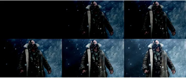
Fade-In
A fade-in process is characterized by a progressive appearing of a shot. The first frame of the fade-in is a monochromatic frame and it progressively shows the first images of the shot. An example of a fade in effect is shown in Figure 3.2
Figura 3.2: A fade-in transition
Fade-Out
A fade-out effect is characterized by a progressive darkening of a shot until the last frame becomes completely black. An example of a fade-out effect is shown in Figure 3.3
Dissolve
The dissolve is characterized by a progressive change of a shot Si into a shotSi+1 with
Theoretical Fundamentals 23
Figura 3.3: A fade-out transition
frames of Shot Si+1 to create the transition. An example of a fade-out effect is shown in
Figure 3.4
Figura 3.4: A dissolve transition
3.3 Image Descriptors
A video is a rich container of visual information. This type of information is used by many techniques to segment the video and even to detect and recognize objects and events. In order to summarize a video, the approach relies on the objects contained in the video and their features.
Some of the most popular features are: color, shape, movement, texture, etc. They are extracted and stored in a feature vector for later use.
3.3.1 Color Histogram
24 Theoretical Fundamentals
Saturation and brightness Value), etc. A color histogram represents the distribution of colors in an image. A histogram is obtained by splitting the range of the data into equal-sized bins (class-intervals), each bin representing a certain intensity value range.
Let f(x, y) be a color image (frame) of size M⇥N, which consists of three channels f = (I1;I2;I3). In order to compute a histogramhc(f, b), each pixel in the image (frame) f is analyzed and is assigned to its corresponding b th bin depending on the pixel intensity. The final value of a bin is the number of pixels assigned to it. Equation 3.1 gives a formal definition of this procedure.
hc(f, b) =
1 M⇥N
XM−1
x=0
XN−1
y=0
8
<
:
1 if f(x, y) in binb
0 otherwise (3.1)
RGB Histogram
In the RGB color space, the RGB histogram is computed by using a combination of three 1-D based histograms, one for each of the RGB color channels (Red, Green and Blue).
Hue Histogram
In the HSV color space, using only the Hue histogram has been very popular. The reason is that the Hue histogram is attributed to give more robust information concerning light intensity, reflecting scale-invariant and shift-invariant (de Sande, Gevers and Snoek 2010, de Sande, Gevers and Snoek 2008).
Using color histograms as image descriptors have several advantages. They are invariant to image rotation and change slowly under the variations of viewing angle and scale (Swain 1993). Another important advantage is its low computational cost, it can be calculated with simple and fast operations.
Theoretical Fundamentals 25
3.3.2 Projection Histograms
Another resource that has been used as a visual descriptor is projection histograms. A projection can be defined as the operation of mapping an image into a one-dimensional vector. For 2D images, the resulting vector is called the projection histogram. The values of the histogram are the sum of the pixels along a particular direction (Trier, Jain and Taxt 1996). Two types of projection histograms can be defined, horizontal and vertical. Considering an image f(x, y), the horizontal histogram will sum the pixels projected onto the vertical axis x as we can see in Equation 3.2. On the other hand, the vertical projection histogram is the sum of the pixels projected onto the horizontal axis y as shown in Equation 3.3.
Mhor(y) =
1 x2 x1
Z x2
x1
f(x, y)d(x) (3.2)
Mver(x) =
1 y2 y1
Z y2
y1
f(x, y)d(y) (3.3)
3.3.3 Scale-Invariant Feature Transform (SIFT)
SIFT is a popular algorithm in computer vision. It was proposed by Lowe (1999). It is an algorithm useful to detect and describe local features in images, it has been used in many application such as object recognition, robotic mapping, 3D modeling, gesture recognition, video tracking, individual identification.
In video summarization, some methods have based their analysis on object detection and recognition. The objects in the video can appear in any location and can also appear at different scales due to zooming effects. The SIFT descriptor is proposed due to its invariance to:
26 Theoretical Fundamentals
We now present the different parts of the algorithm.
Construction of the scale space
In this initial step, internal representations of the original image are created to ensure scale invariance. This is done by generating a “scale space”. To create a scale space, progressively blurred out images are generated from the original image. Then, the original image is resized to half its size, after that more blurred out images are generated again. This process repeats as many times as it is necessary. Each level of resized images are called octaves.
It must be noted that the number of octaves and scales produced have a direct relation to the original image size. The author of SIFT suggests that 4 octaves and 5 blur levels are ideal for the algorithm.
In order to blur the image, a convolution of the gaussian operator and the image is performed. A Gaussian blur operator is applied to each pixel, the final result is a blurred image. Equation 3.4 defines this operation.
L(x, y, ) =G(x, y, )⌦f(x, y) (3.4)
Where:
• Lis the resulting blurred image.
• Gis the Gaussian Blur operator defined in Equation 3.5. • f is the image to be processed.
• x, y are the location coordinates of the pixel. • defines the amount of blur to be applied. • ⌦is the convolution operation.
G(x, y, ) = 1 2⇡ 2e
−(x2+y2)/2σ2
Theoretical Fundamentals 27
Laplacian of Gaussian
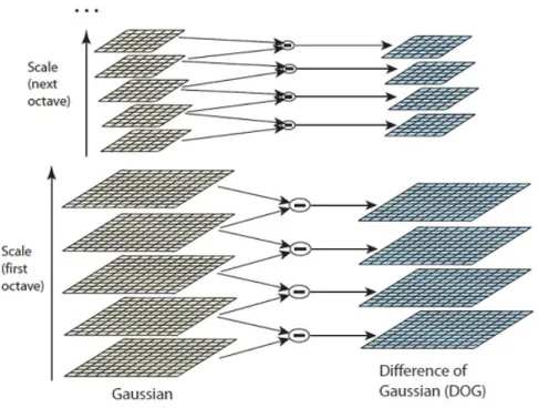
In this step, the edges and corners on the image are located, these will be used for finding keypoints. The algorithm could use the Laplacian of Gaussian directly to do this, but it is computationally expensive. To overcome this problem the method proposes a different procedure. They propose to use the scale space previously computed, then calculate the difference between two consecutive scales. This is actually a difference of Gaussians (DoG) as shown in Figure 3.5. The resulting image from the DoG is approximately equivalent to the Laplacian of Gaussian. So the operation becomes a simple difference of images instead of a more complicated procedure.
Figura 3.5: Difference of Gaussians
The DoG is given by Equation 3.6.
D(x, y, ) = L(x, y, ki ) L(x, y, kj ) (3.6)
28 Theoretical Fundamentals
Locate Potential keypoints
In this step, the possible keypoints using the resulting image explained in Subsection 3.3.3 are located. This process has two parts:
1. Locate maxima/minima in DoG images: this is done by iterating each pixel and checking its corresponding neighbors. The current image and the images above and below it are used. In Figure 3.6, the X marks the current pixel to be processed and the circles mark the neighbors. The evaluated pixel has total of 26 neighbors, the current pixel is marked as a keypoint if it is the greatest of the least of all the 26 neighbors. After doing this, several maxima and minima points are found, but they are an approximation. The real maxima and minima points are located somewhere inside the pixel. To find the actual position the subpixel location needs to be calculated.
Figura 3.6: Locating maxima/minima in DoG images
2. Subpixel maxima/minima: using the detected pixel data, the subpixel location is computed. This is done by the Taylor expansion of the image around the approximate keypoint. Equation 3.7 defines the Taylor series expansion. This will accurately determine the position of the keypoint
D(x) = D+@D
T
@x x+ 1 2x
T@2D
Theoretical Fundamentals 29
Filter Edge and Low Contrast Responses
At this point, some of the several detected keypoints might not be useful. Two things can happen, either some of them are located on an edge, or they may not have enough contrast. If this things happen, then the keypoint is considered to be irrelevant and should be ignored.
To remove a low contrast feature, a threshold th is used. If the magnitude of the intensity in the DoG image is less than th, then the keypoint is ignored.
To remove edges, two gradients are calculated at the keypoint. The objective is to search for corners and they are detected when both gradients are big. In order to do this, the Hessian matrix defined in Equation 3.8 is used. If the evaluated keypoint is not detected as a corner, then it is ignored.
M =⇣Dxx Dxy Dxy Dyy
⌘
(3.8)
Assign Keypoints Orientations
In this step, the gradient directions and magnitudes around each detected keypoint are collected. Then, the most prominent orientation in that region is computed. Finally, this orientation is assigned to the keypoint. The size of the region will depend on the image scale.
Generate SIFT features
30 Theoretical Fundamentals
3.3.4 A SIFT Descriptor with Color Invariant Characteristics
(CSIFT)
One big challenge for a feature descriptor is to be robust to imaging conditions. The descriptor should provide features that are invariant to geometrical variations like rotation, translation, scaling, etc. Many approaches, such as SIFT, use local features to be geometrical invariant, but they avoid using colored images since it can add certain degree of difficulty.
The original SIFT only uses information of gray scale images. However, color can provide important information in object description. Abdel-Hakim and Farag (2006) propose CSIFT, their approach uses a color invariant space to build the SIFT descriptor instead of the traditional gray scale.
CSIFT is a local invariant feature descriptor that allows the descriptor to be more robust to color variations. The CSIFT algorithm uses the same steps as in the SIFT algorithm. The interest points detection is performed by a difference-of-Gaussian for the input image in different scales. The difference is that the working space is the result of a color invariance model.
Geusebroek, Van den Boomgaard, Smeulders and Geerts (2001) propose the color invariance method, which is suitable for modelling non-transparent/traslucent materials. To calculate its values from the RGB color space, a Gaussian color model is used. This model represents the spectral information and the local image structure. Abdel-Hakim and Farag (2006) propose to compute the values from the product of two linear transformations. The implementation of the Gaussian color model using the RGB values can be calculated using Equation 3.9.
0 B B B @ ˆ E ˆ Eλ ˆ Eλλ 1 C C C A = 0 B B B @
.06 .63 .27 .3 .04 .35 .34 .6 .17
1 C C C A 0 B B B @ R G B 1 C C C A (3.9)
where ˆE,Eˆλ,Eˆλλ are the computed color invariants.
Theoretical Fundamentals 31
3.3.5 HUESIFT
Weijer, Gevers and Bagdanov (2006) introduced the idea of concatenating the Hue histogram to the SIFT descriptor. Consequently producing the HUESIFT descriptor, which was later used by (de Sande, Gevers and Snoek 2010). Similar to the hue histogram, it shares the same properties. This means that the HUESIFT descriptor is scale-invariant and shift-invariant. However, one important drawback is that, unlike the SIFT descriptor; the HUESIFT is not invariant to illumination color changes. This behavior was noted by de Sande, Gevers and Snoek (2008).
3.3.6 SURF: Speeded-Up Robust Features
Bay, Ess, Tuytelaars and Van Gool (2008) propose SURF (Speeded-Up Robust Features), it is a fast and robust algorithm for local similarity invariant image representation. SURF can be used in object recognition and tracking. Its fast computation makes it suitable for real-time applications.
1. Scale-space approximation via box filters. In order to make the features invariant to scale, a scale-space representation is usually computed using Gaussian convolutions of the image at certain scales. SURF approximates the Gaussian Kernel and spatial derivatives using rectangular functions. The approach treats these functions as box filters. Doing this, makes the convolution complexity linear and therefore faster. The resulting scale-space representation using box filters is very similar to the one generated by Gaussian kernels. As in Gaussian kernels, a scale parameter is defined to create different scales of blurred images.
2. Interest points detection:
To detect the interest points, SURF follows three steps:
• Feature detection. To detect scale-invariant features a scale-normalized second order derivative on the scale space representation is used. SURF approximates this using a scale-normalized determinant of the Hessian (DoH) operator. • Feature selection. Once the DoH operator has been applied to the scale-space
32 Theoretical Fundamentals
maxima points, the algorithm uses a threshold tH on the response of the DoH
operator. This is applied to every local maxima point, and a set of interest point candidates is generated.
• Scale-space location refinement. In order to refine the location of the interest points, a second order interpolation is used.
• Storage of the interest points. The interest points detected are saved with information about their position (x, y) and their respective .
3. Local descriptors construction. Equation 3.10 formally describes the interest points detected.
{Mi : (xi, yi, i)}i=1,2,...N (3.10)
For each interest pointMi, the local orientation is computed from the local
distri-bution of the gradient orientation, which is obtained by the convolution with box filters. An orientation✓i is computed.
To construct the SURF descriptor, for each interest point a 16⇥4 vector is computed. The vector represents normalized gradient statistics corresponding to the scaled and oriented neighborhood of the interest point.
3.3.7 Space-Time Interest Points (STIP)
Laptev (2005) proposes an algorithm to detect spatio-temporal events using space-time interest points. The features contain not only space but also time information. Interest points are detected using the Harris operator. The algorithm looks for structures with significant local variations in terms of space and time.
Spatio-Temporal Interest Point Detection
To detect interest points in the spatial domain, an image can me modeled by a linear scale-space representation. The image can be defined by fsp :R2 !R. A functionLsp is
used to represent the linear scale-space, whereLsp :R2⇥R
+!R is defined in Equation
Theoretical Fundamentals 33
Lsp(x, y; l2) =gsp(x, y; l2)⇤fsp(x, y) (3.11)
where the image fsp is convolved with a Gaussian kernel of variance 2
l and gsp is defined
in Equation 3.12
gsp(x, y; 2l) = 1
2⇡ l2exp( (x
2+y2)/2 2
l) (3.12)
The algorithm applies the Harris operator to detect the interest points. The idea is to find spatial locations where fsp has significant changes in both directions. To do this,
a second moment descriptor µsp is used. Then, the algorithm calculates the eigenvalues
1, 2 (where 1 2 ) of µsp. If 1, 2 have large values, then an interest point is
detected. Equation 3.13 defines the operator to obtain the Harris interest points.
Hsp = 1 2 k( 1+ 2)2 (3.13)
where k is a constant, in the literature the value used is usually k = 0.04
To detect interest points in the spatio-temporal domain, Laptev (2005) proposes an operator that is sensitive to events in temporal image sequences at specific locations considering space-time information. The interest points detected will represent values in local spatio-temporal volumes, they are required to have certain variation along the spatial and the temporal directions.
A functionf :R2⇥R!R is used to model the spatio-temporal image sequence. The
algorithm generates the linear scale-space representation L:R2⇥R⇥R2 !R, using a
Gaussian kernel to convolvef. The Gaussian kernel has spatial variance 2
l and temporal
variance⌧l2. This representation is defined in Equation 3.14.
L(x, y, t; l2,⌧l2) = g(x, y, t; 2l,⌧l2)⇤f(x, y, t) (3.14)
34 Theoretical Fundamentals
g(x, y, t; 2l,⌧l2) = p 1
(2⇡)3 4
l⌧l2
⇥exp
✓
(x2+y2)
2 2
l
t2
2⌧l2
◆
(3.15)
As in the spatial domain, a spatio-temporal second moment matrix is used. The matrix is composed by a first order spatial and temporal derivatives, these values are averaged using a Gaussian functiong(x, y, t; 2
i,⌧i2).
µ=g(x, y, t; i2,⌧i2)⇤
0 B B B @ L2
x LxLy LxLt
LxLy L2y LyLt
LxLt LyLt L2t
1 C C C A (3.16)
The algorithm uses the integration scales 2
i,⌧i2, which are related to the local scales
2
l,⌧l2, where 2i =s l2, ⌧i2 =s⌧l2, and s represents the scale.
The first order derivatives can be calculated using the following formulas: Lx(x, y, t; 2l,⌧l2) = @x(g⇤f)
Ly(x, y, t; l2,⌧l2) =@y(g⇤f) Lt(x, y, t; l2,⌧l2) =@t(g⇤f)
Then, the eigenvalues 1, 2, 3 ofµare calculated. (Laptev 2005) proposes to extend
the Harris corner function. The extended function is defined in Equation 3.17.
H = 1 2 3 k( 1 + 2 + 3)3 (3.17)
where the constant k is usually set to the value k ⇡0.005.
Theoretical Fundamentals 35
3.3.8 Histograms of Oriented Gradients (HoG)
Dalal and Triggs (2005) propose the Histogram of Oriented Gradient descriptors. The basic idea of this descriptor is that using the distribution of intensity gradients or edge directions, the local object appearance and shape can be described.
The algorithm first creates cells by dividing the image into small connected regions, each cell will have a set of associated pixels within it. Then, for each of the cells the algorithm computes a histogram of gradient directions or edge orientations. The descriptor is formed by the combination of these histograms. To further improve the descriptor, a normalization can be performed to provide the descriptor a better invariance to changes in illumination. To do this normalization, the algorithm takes a block which is a larger region of the image and measures the intensity. The obtained value is used to normalize all the local histograms that belong to cells that are within the block.
The algorithm is further described below:
Gamma/Colour Normalization
This is a pre-processing step. A global image normalization is performed in order to reduce the influence of illumination effects.
Gradient Computation
In this step, the gradient values are calculated. Dalal and Triggs (2005) propose to apply a simple 1-D centered mask, which according to their experiments gave the best results. The used masks are: [ 1,0,1] and [ 1,0,1]T. More complex masks, such as 3⇥3 sobel
masks where evaluated by the authors but the results obtained with them are not as good as the ones obtained with the simple 1-D masks.
Orientation binning
36 Theoretical Fundamentals
weight can be computed from the gradient magnitude, or some function of the magnitude (square, square root, clipped). Nevertheless, gradient magnitude generally produces the best results according to the authors. Cells can either be of rectangular or radial shape.
Normalization and Descriptor Blocks
Normalization gives the descriptor better invariance to illumination, shadowing, and edge contrast. To do this, local groups of cells called “blocks” are normalized. The algorithm accumulates a measure of local histogram “energy” over the blocks, the value calculated from this is used to normalize the different cells that belong to the block.
To normalize a block, letv be the non normalized vector containing the histograms in a block, kvkk be its k norm for k = 1,2 and ✏ a constant. The normalization can be
calculated using several schemes such as: L2 norm, L1 norm, L1 sqrt. Equations 3.18, 3.19 and 3.20 defines each of these normalizations respectively.
• L2 norm
v ! p v
kvk2 2+✏2
(3.18)
• L1 norm
v ! v
kvk1+✏
(3.19)
• L1 sqrt
v !pkvk1+✏ (3.20)
The authors found that normalizations L2 norm and L1 sqrt provide similar performance, andL1 norm provided less reliable performance.
Theoretical Fundamentals 37
Finally, the algorithm collects the HoG descriptors from all the blocks covering the detection window into a integrated feature vector.
3.4 Classification
Classification is one of the most frequent tasks to be solved when taking decisions. The problem appears when certain object needs to be associated to some class. To do this, the models base their analysis in the features and possible relations of the object. There exist two types of classification: supervised classification and unsupervised classification.
In the supervised classification, some previously labeled patterns are at hand. For these patterns, the classes they belong to are already known. The problem is to classify new unlabeled patterns. Therefore, the labeled patterns help us to train the classification model, once the model has been trained it can be used to classify new objects. The problem is that in real life, that previous information is not always present.
The unsupervised classification is useful when no previous class information is present. This type of classification is also known as clustering. The clustering model is widely used in video summarization. The patterns are feature vectors that represent multidimensional points, the clustering models use these feature vectors to compute the similarity between them and thus create and classify the patterns in classes.
3.4.1 K-means
The K-means has been one of the most popular unsupervised clustering algorithms, it was proposed by MacQueen (1967). The procedure needs to know a priori the number of clusters k, a cluster consists of feature vectors with similar characteristics that is represented by a centroid. Initially, k centroids are located at random positions.
38 Theoretical Fundamentals
j =Xk
j=1
Xn
i=1kx (j)
i cjk2 (3.21)
where kx(ij) cjk2 represents the distance between the element x(ij) and the centroid cj
Unfortunately, the K-means algorithm will not always find the most optimal clas-sification. Another disadvantage is its sensitiveness to the initial centroids position. Consequently, the algorithm will not always produce the same result for a data set.
3.4.2 X-means: Extending K-means with E
ffi
cient Estimation
of the Number of Clusters
The original K-means algorithm has been very popular due to its simplicity and quick implementation. However, the K-means algorithm has three shortcomings that are overcome by X-means algorithm (Pelleg and Moore 2000). First, it can be slow due to repetitive interactions. Second, the number of clusters has to be knowna priori, meaning the user has to input the quantity of classes. Finally, Pelleg and Moore (2000) stated that when a fixed value K is used, the algorithm finds worse local optima compared to results obtained when the value K is dynamically modified.
Pelleg and Moore (2000) propose the X-means algorithm to quickly estimate theK number of clusters. The user is required to input a reasonable range of values of K, minimum and maximum. Then, the algorithm uses this range to select the best set of centroids and the best value forK. The model selection criterion used is the Bayesian Information Criterion (BIC).
The definitions used are:
• µj coordinate of thej th centroid.
• ithe index of the centroid that is closest to he i th data point. • D the data set.
• R=|D|.
• M number of dimensions.
Theoretical Fundamentals 39
The X-means algorithm consist of the following operations: X-means:
1. Improve Parameters 2. Improve Structure
3. If K > Kmax Stop and generate the best scoring model.
Else Goto Step 1
These operations are further explained below:
1. Improve Parameters. This is a simple operation, the algorithm executes a conventionalK means.
2. Improve Structure. This operation is the core of the algorithm. It finds out if new centroids should be created and also defines the location of the new centroids. The strategy is the following:
• Split each centroid (parent) into two children
• They are moved to a distance that is proportional to the size of the region in the opposite direction.
• Each parent has a region, a local K means is executed with K = 2.
• A model selection (BIC) is executed on the recently created pairs of children. The model helps the algorithm decide whether to create new centroids or not to. Given the data D and a set of alternative models Mj (these models are the
solutions with different values of K ). The BIC score can be calculated using 3.22.
BIC(Mj) = ˆlj(D) pj
2 · logR (3.22)
where ˆlj(D) is the log-likelihood of the data according to the j th model. pj
is the number of parameters in Mj, it is the sum of K 1 class probabilities.
40 Theoretical Fundamentals
• All stable-state information is saved. Therefore, the algorithm no longer re-computes stable values, reducing the number of calculations in each iteration. The main contribution is to incorporate the model selection into their algorithm. Using statistically-based criteria to make local decisions helps the algorithm find the optimal K value.
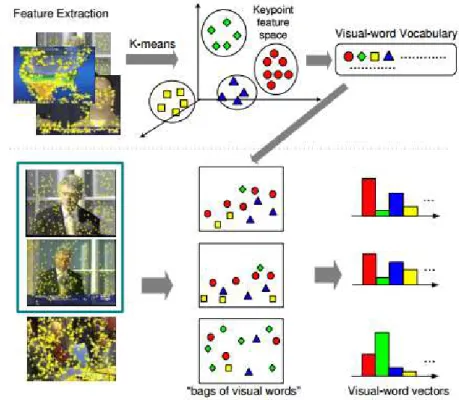
3.5 The Bag-of-Words model
The bag-of-words model (BoW), was originally proposed for text processing. It was applied to simplify the representation used in natural language processing and information retrieval. In computer vision, the model was adapted by considering image features as words. To represent an image using BoW model, an image can be treated as a document. Three operations are executed: Feature detection, feature description and codebook generation.
• Feature representation: Feature detection and feature description.
This is usually done by applying a keypoint detection algorithm and a keypoint descriptor. One of the most popular descriptors is the SIFT descriptors. The result from this operation is a set of feature vectors, one for each detected keypoint. • Codebook generation It is usually achieved by performing K-means clustering over
all the vectors. Codewords are then defined as the centers of the learned clusters. The number of the clusters is the codebook size.
After performing these operations, the visual word vocabulary is defined. Then, future images can be described by the occurrences of the visual words according to our visual word vocabulary. This is done by computing a histogram of occurrences (visual word vectors). In 3.7, a general overview of the Bag-of-Words approach is presented.
3.6 Final considerations
Theoretical Fundamentals 41
Figura 3.7: The Bag-of-Words model
Cap´ıtulo 4
Proposed Method
In this chapter, a method for static video summarization is described. The presented method is used in this dissertation to generate the different video summaries. Additionally, an evaluation model is reviewed to estimate the quality of the generated summaries. The chapter is organized as follows: in Section 4.1 each of the steps for summarizing videos is described. In Section 5.3, the model for evaluating video summaries is presented.
4.1 Proposed Method for Summarizing Videos
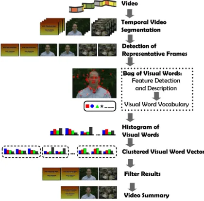
In Figure 4.1, we present a general overview of our proposed method. Initially, a temporal segmentation procedure is executed. As a result, several shots are detected. Then, each shot is clustered. This is done to detect frame samples from each shot. Later, for each of the frames previously detected, a feature description procedure is applied. Afterward, a Bag-of-Words (BoW) approach is adopted. The detected local features are clustered to generate our Visual Word Vocabulary. Next, the histograms of occurrence of visual words are created for each frame of the detected frame samples. The histograms of occurrence are clustered, the method finds the frames that are near to each cluster’s centroid. The frames that represent the centroids are considered as keyframes. The method filters the results to eliminate possible redundant keyframes. Finally, the keyframes are ordered in chronological order. The final result is the video summary.
44 Proposed Method
Figura 4.1: Method for Summarizing Videos
4.1.1 Temporal Video Segmentation
Proposed Method 45
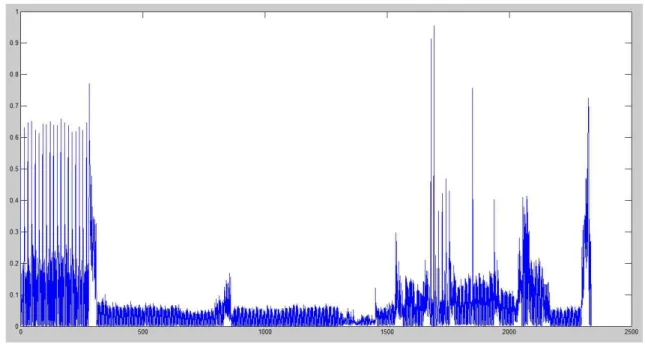
In Figure 4.2, a dissimilarity vector is shown for a video. As we can see, usingth = 0.4 will detect several false shot cuts. In order to overcome this problem, a procedure is executed to refine the dissimilarity vector.
Figura 4.2: A dissimilarity vector computed from videoHCIL Symposium 2002 - Introduction, segment 01
The procedure works as follows: each of the values in the dissimilarity vector is analyzed. Each value becomes a pivot when evaluating the dissimilarity vector. Then, a neighborhood of values around the pivot is taken, excluding the value of the pivot. The maximum value mv of the neighborhood is calculated. If the value of the pivot v is greater thanmv, the value of the pivot is modified by applying Equation 4.1.
si =
8
<
:
vi−mvi
vi if vi > mvi vi otherwise
(4.1)
where i is a position in the dissimilarity vector,si is the computed value, vi is the value
of the pivot and mvi is the maximum value of the neighborhood around the pivot.
46 Proposed Method
To know the number of segments present on the video, the method simply counts the number of abrupt changes.
This type of segmentation is very effective and not computationally expensive. Howe-ver, there is one shortcoming. Videos usually have visual effects such as fade in, fade out and dissolves. Figure 4.4 shows a dissolve effect.
A dissolve effect can produce distorted images, these type of images have a great impact in the discriminative power of a descriptor. An frame that is produced during the dissolve transition will produce a lot of spurious keypoints. These false keypoints will eventually affect the summarization process. To overcome this problem, the method identifies the portions of the video where this effect happens. Once these portions are detected, they are excluded of any posterior analysis.
To detect the possible dissolve effect in the video, our method first compute the variance in each frame of the video and put it in a vector. Figure 4.5 shows the resulting variance vector for a video. Dissolve effects are located in the valley areas in the variance vector. Therefore, the method uses a procedure based on (Won, Chung, Kim, Choi and Park 2003, Camara Chavez, Precioso, Cord, Phillip Foliguet and de A. Araujo 2007) to detect the valleys areas in the variance vector and consequently find the portion of video where a dissolve effect occurs.
At this point, the method has detected the shot boundaries and therefore segmented the video. Furthermore, by detecting the dissolve effects the method can exclude not relevant portions of video that can actually affect the performance of the summarization method.
4.1.2 Detection of Representative Frames
Proposed Method 47
4.1.3 Bag of Words (BoW)
Our method uses the Bag-of-Words (BoW) approach to summarize videos. To adopt the approach, an image can be considered as a document.
The “words” are the visual entities found in the image. They will describe the object and therefore represent our semantic entities. Using their information we can perform a semantic summarization based on the objects of the video.
The Bag-of-Words (BoW) approach consists of three operations: feature detection, feature description and visual word vocabulary generation. Many local descriptors, such as SIFT, can be used for feature detection and description. A visual word vocabulary is generated from the feature vectors obtained during the feature detection process, each visual word (codeword) represents a group of several similar features. The visual word vocabulary defines a space of all entities occurring in the video, it can be used to semantically summarize the video based on the entities present on it.
Feature Detection and Description
Images can be described by global features, such as: color, texture, etc. But they can also be described by the objects contained within it, using local descriptors. A feature detection and description algorithm can be computed on an image to detect and describe the interest points of the objects. Such algorithm must be robust to geometrical transformations, noise and illumination variances.
For this dissertation, the local descriptor extracts the features for each of the frames detected in the previous step. The method can use any local descriptor, such as:
• SIFT • SURF • CSIFT • HOG • HUESIFT
48 Proposed Method
Visual Word Vocabulary
A word vocabulary, also known in the literature as the “codebook”, defines the “codewords” used in the Bag-of-Words. A “codeword” represents a group of feature vectors that share similar characteristics.
To compute the “codewords” all feature vectors are grouped and classified using a clustering algorithm. Any clustering algorithm, such as K-means, can be used. Then, the “codeword” is defined as the center of the detected cluster.
The “codebook” size establish the number of visual words. This value determines the number of clusters to be found. For this dissertation, the “codewords” are the visual words and the “codebook” is the entire visual word vocabulary. Correctly establishing the number of visual words is still a open problem.
4.1.4 Histogram of Visual Words
A histogram of visual words is created by counting the occurrence of the visual words. For each representative frame, the local image features are used to find the visual words that occur in the image. These occurrences are counted and arranged in a vector. Consequently, each representative frame will have an associated vector of visual word occurrences (visual word vector).
4.1.5 Visual Word Vectors Clustering
Finally, the method uses all the visual word vectors recently obtained and applies the X-means algorithm. Frames with similar visual entities are grouped together. Then, for each cluster, the nearest frame to the centroid is chosen as the “keyframe”. All the detected “keyframes” are ordered according to their time of appearance and they represent the video summary or storyboard. By doing it, we have grouped together the most representative frames of the video taking into consideration the semantic information (visual entities) contained in them. This ensures that the final video summary contains
Proposed Method 49
4.1.6 Filter Results
This final operation tries to eliminate possible duplicated “keyframes”. A pairwise similarity measure is calculated from color histograms of consecutive keyframes. Then, keyframes with high similarity are removed from the final video summary. The method uses a threshold of value 0.5 to define a high similarity between two color histograms, as in (de Avila, ao Lopes, da Luz and de Albuquerque Ara´ujo 2011).
4.2 Final Considerations
50 Proposed Method
Figura 4.3: A refined dissimilarity vector computed from video HCIL Symposium 2002 -Introduction, segment 01
Proposed Method 51