Universidade Nova de Lisboa
Thesis, presented as part of the requirements for the Degree of Doctor of
Philosophy in Economics
Firm and Consumer Behaviour in Energy Markets
Marta Proença de Almeida Oliveira Rocha
657
A Thesis carried out on the Ph.D. Program in Economics, under
the supervision of Prof. Steffen Hoernig
Abstract
This dissertation consists of three essays on the study of firm and consumer behaviour motivated by the energy markets. The first chapter studies whether a firm with better information than their rivals about the customers in the market can use that information to earn more profits. The second chapter studies whether a profit-maximising firm would want to induce positive consumption to a consumer that has self-control issues. The third chapter analyses empirically whether self-control issues can explain the problem of self-disconnection that persists in prepayment energy meters.
Acknowledgements
This thesis would not have been possible without the support and encouragement of a great number of people and institutions. First and foremost, I would like to express my gratitude to my advisor, Steffen Hoernig, for his guidance that was crucial for the development of this thesis and for challenging my thinking. I am grateful to Fundação para a Ciência e Tecnologia that funded four years of my PhD.
I am grateful to David Newbery who has given me the opportunity to visit Cambridge for two times. The vibrant academic environment in Cambridge gave me strength and desire to continue learning. I really felt that I belonged to the Faculty and the EPRG and I benefited greatly from the seminars, meetings and discussions with students and lecturers. Thank you Michelle Baddeley and Michael Pollitt for believing in me and for pushing me to start the self-disconnection project. I would like to thank British Gas for their great support and collaboration. I am deeply grateful to Michelle Baddeley who always believed in me and for continuously giving me strength to continue my research. I am grateful to Hans Keiding who welcomed me during my stay at University of Copenhagen. I have benefitted greatly from all the seminars and lectures at Nova. A grateful thank you to all the participants from the PhD research group, RES and QED conferences who gave me invaluable comments and suggestions. A special thank you to my PhD colleagues, especially Pedro and João who made me laugh when I needed it most.
Contents
Introduction ix
1 Contracting in a market with differential information 1
1.1 Introduction . . . 1
1.2 Related Literature . . . 3
1.3 The Model . . . 5
1.3.1 No Differential Information . . . 9
1.3.2 Differential Information . . . 11
1.3.3 Market Structure and Social Surplus . . . 13
1.4 Robustness Analysis . . . 15
1.4.1 Number of customers . . . 15
1.4.2 Number of firms . . . 16
1.4.3 Number of types . . . 17
1.5 Conclusion . . . 18
1.6 References . . . 20
1.7 Appendix . . . 22
2 Contracting in a market with self-control 28 2.1 Introduction . . . 28
2.2 Related literature . . . 31
2.4 Analysis . . . 37
2.4.1 Agent’s choices . . . 37
2.4.2 Consumption constraints . . . 38
2.4.3 The principal’s problem . . . 41
2.4.3.1 Single contracts . . . 41
2.4.3.2 Menu of contracts . . . 45
2.5 Discussion . . . 49
2.5.1 Model without the naïve type . . . 49
2.5.2 Impact of naiveté on the principal’s expected profit . . . 50
2.5.3 Impact of naiveté on the agent’s utility . . . 51
2.6 Conclusion . . . 52
2.7 References . . . 54
3 Addressing self-disconnection among prepayment energy consumers: A be-havioural approach 56 3.1 Introduction . . . 56
3.2 Background on prepayment energy . . . 59
3.3 A mechanism to minimise self-disconnection . . . 61
3.3.1 Commitment contract . . . 62
3.3.2 Reminder/Feedback on consumption . . . 65
3.4 Data . . . 67
3.5 Estimation Strategy . . . 77
3.6 Results . . . 81
3.6.1 Self-disconnection and Emergency Credit . . . 81
3.6.2 Worried . . . 84
3.7 Discussion . . . 89
3.8 Conclusion . . . 92
3.9 References . . . 93
List of Figures
List of Tables
3.1 Main features of the commitment contracts . . . 64
3.2 Survey sample: control variables . . . 68
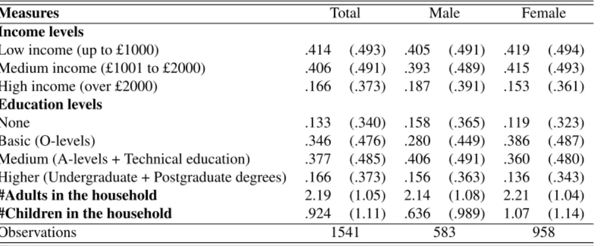
3.3 Descriptive statistics: demographic characteristics . . . 69
3.4 Distribution of emergency credit and self-disconnection . . . 70
3.5 Correlations between variables characterising individual heterogeneity . . 74
3.6 Distribution of the different plans . . . 76
3.7 Seemingly unrelated bivariate probit: emergency credit and self-disconnection 83 3.8 Probit: self-control variables on worried . . . 86
3.9 Multinomial logit: preferred plan (base comparison: “None of the options”) 88 3.10 Cross tabulation: preferred saving plan vs. low-income . . . 90
3.11 Cross tabulation: preferred saving plan vs. self-disconnection . . . 90
A1 List of main variables . . . 97
A2 Cross tabulation between inconvenience of top up and self-disconnection . 98 A3 Cross tabulation between inconvenience of top up and self-disconnection . 98 A4 Cross tabulation between saving behaviour and self-disconnection . . . . 98
A5 Cross tabulation between spare cash and low-income . . . 99
A6 Distribution of goal achievement questions . . . 101
A7 Low Goal Achievement: mean characteristics . . . 102
A8 Medium Goal Achievement: mean characteristics . . . 103
Introduction
In many market situations, firms face the problem of the heterogeneity of consumers’ tastes or types. Even if a firm knows the distribution, it does not know the type of any given customer. However, a firm can design a menu of contracts that is an incentive mechanism in which consumers are induced to reveal their type by their self-selection in the menu. This dissertation builds on incentive theory from different perspectives, although not being entirely in the area of incentive theory.
This dissertation uses energy markets as a motivation for the different issues analysed. Energy markets are surprisingly understudied from an economic point of view and have been evolving significantly with a number of new problems. Such an example is an emerging set of information and communication technologies in the electricity sector, called smart grid, that has allowed for innovative forms of metering. The debate over the smart grids has deserved a considerable engineering attention, but it is still an open issue in economic terms. In particular, there is still some debate around the sensitivity of data on consumers’ energy usage and who should hold this data. Discussions about potential discriminatory behaviour have already been made by energy regulators. This raises the question whether it is, in fact, profitable for a firm that has access to consumers’ data energy usage to share it with particular third parties.
of information, we introduce a framework of two firms supplying a good composed of many commodities that compete in prices, which have access to the same technology and where customers have fixed demand. We are interested in the equilibrium outcomes under no differential information and under differential information. We show that, under no differential information, both firms equally share the customers and types of customers, charge the same payments and obtain zero profits. Under differential information, we as-sume that access to better information allows the better informed firm to attract specific customers. Access to better information gives the better informed firm a first customer contact advantage. The uninformed firm can only offer a menu of tariffs without being able to pre-identify the customer’s type. Nonetheless, the uninformed firm can access the market, not allowing the better informed firm to make positive profits. We find that better information does not give a firm an advantage or disadvantage, that is, it obtains the same equilibrium profit as the uninformed firm.
Current energy meters, as opposed to smart meters, also present some issues. One of those is significantly related with prepayment meters which is a payment method where the payment is made before the actual consumption. That is, consumers have to pay for electricity and/or gas (immediate costs) before they consume it (delayed benefits). Moreover, consumers must plan in advance their future consumption. This planning, or lack of it, may lead to self-disconnection, which happens when consumers exhaust all available credit in their meter and are left without supply of energy for a certain period. Self-disconnection has serious consequences for the wellbeing of consumers. Likewise, it generates costs for the energy suppliers since it may contribute to lower energy con-sumption, higher debt levels, and higher costs related to reconnection of energy supply. This self-disconnection can be explained by the presence of self-control issues that can lead a consumer to under-consume.
self-control”, studies theoretically whether a profit-maximising firm would want to in-duce positive consumption to a consumer that is time-inconsistent and is unaware of his degree of time inconsistency. The literature on behavioural economics defines this type of consumer as naïve, in which differs from a sophisticated type in the sense that the latter is aware of his degree of time inconsistency. The firm/principal cannot observe the type of the consumer/agent at the contracting stage. In order to make any payment, the agent needs to make a saving decision and incur a savings effort cost. The agent’s marginal utility of consumption is affected by a shock after the contracting stage. We study two specific contract forms: a pay-in-advance contract that involves a payment at date 0 and a payment at date 1, and a pay-in-advance contract that only involves a payment at date 1. We show that the principal can induce positive consumption to all types, but there is a trade-off between increasing efficiency and decreasing information rent when offer-ing a menu of contracts. We also study the impact of the naïve type on the remainoffer-ing types’ utilities and on the principal’s expected profit and show that the principal may have incentives to educate the naïve type.
The final essay, “Addressing self-disconnection among prepayment energy consumers: A behavioural approach”, analyses empirically whether self-control issues can explain the problem of self-disconnection that persists in prepayment energy meters. We study a mechanism composed of a commitment contract and a reminder in order to minimise the number of self-disconnections. We design and implement a survey to energy con-sumers that use a prepayment meter in the UK. We show that self-control plays a role in self-disconnection and we are able to identify, in our sample, those consumers who benefit from a commitment contract. Moreover, we find a demand for commitment and an opportunity to save among those consumers who need a commitment contract.
Chapter 1
Contracting in a market with
differential information
1
1.1
Introduction
The recent advanced infrastructures in the energy sector based on smart meters are now capable of real lifetime pricing and remote reading. This has generated a debate in re-lation to the potential sensitivity of data on customers’ patterns that firms will be able to hold once smart meters are fully implemented. Indeed, the major players in the en-ergy markets, such as network providers, suppliers, regulators and customers, recognise the potential sensitivity of data on customers’ energy usage. The Council of European Energy Regulators has already made recommendations over potential discriminatory be-haviour and potential measures of data security (CEER 2015).2 Nevertheless, it is still not clear what is the impact of this new degree of information on competition in the energy markets.
1This is joint work with Thomas Greve.
2This potential discriminatory behaviour can come from a vertical connection between the distribution
The key question posed in this paper is whether a firm with better information about the customers in the market than their rivals can use that information to earn more profit. Although, it might seem intuitive, one cannot claim under generality that access to better information leads to higher profits.
To study the role of information, we introduce a framework of two firms supplying a good composed by many commodities that compete in prices, which have access to the same technology and where customers have fixed demand. We are interested in the equi-librium outcomes under no differential information and under differential information. To answer our research question, we compare the equilibrium profits of both firms in two ways. First, we define information advantage as the difference between the equilibrium profits of the better informed firm and the uninformed firm in the differential informa-tion case. Second, we define informainforma-tion value as the difference between the equilibrium profits of the better informed firm under differential information and under no differential information.
is no information value because the better informed firm has the same equilibrium profit under both cases.
We also analyse whether our results are robust to changes in the number of customers, number of firms and number of types. We show that as long as it is possible to equally divide the number of customers between firms, the symmetric Nash equilibria in pure strategies exist. Under differential information, the exclusionary Nash equilibria exist despite of the number of customers of each type. However, once we increase the number of better informed firms, the exclusionary equilibria exist as long as it is possible to equally divide the number of customers between the better informed firms.
1.2
Related Literature
Cournot. The consequences of differential information arise because the better informed firm can decide to invest more or less in the first stage.
A more related study to the present paper is Einy et al. (2002). It is shown that a better informed firm is rewarded, under Cournot competition, when firms’ technology exhibits constant returns to scale. Chokler et al. (2006) challenge Einy et al. (2002) results and prove that in Cournot duopolies with differentiated products and linear demand and cost functions, the better informed firm earns less profit if both firms have symmetric demand functions. Consequently, one cannot claim, under generality, that better information leads to higher equilibrium profit for the better informed firm. Indeed, we show that in a one-stage Bertrand competition, differential information can lead to no information advantage or disadvantage.
literature by studying personalised pricing in a model with homogeneous goods and with differential information. In particular, we show that although, it is possible for the better informed firm to target customers, that does not allow it to charge higher prices.
The literature on privacy is closely related to the literature on competitive price dis-crimination and on personalised pricing. The literature on economics of privacy has analysed, for example, how firms use past behaviour of consumers to infer their taste and price (see e.g. Fudenberg and Tirole, 2000; Esteves, 2010); and how privacy ac-tions are undertaken by consumers and how consumer information is sold to firms (see e.g. Casadeus-Masanell and Hervas-Drane 2015, Montes et al. 2016 and Taylor and Wagman 2014). This literature has been expanding significantly due to the rise of new technologies and online markets that are able to store consumers’ personal information.3 This also relates to the motivation of our paper in the sense that smart meters will allow for monitoring and recording of electricity consumption on a near real-time basis. Tech-nology will also allow identifying the activities of consumers by matching data on their electricity usage with known appliance load signatures.4
1.3
The Model
Consider an industry where two firms compete in the production of m > 1 different commodities. There is a given finite setA ⇢Rm
+ oftypesof customers, where a type is a
vectora 2 A specifying the demand for each of them commodities. Assume that each commodity is homogeneous.
3
For an overview of the literature on economics of privacy see Acquisti et al. (2016).
4
Suppose that there are only two types of customers,A = {au, ap}, whereau is the uniform type and ap is the peak type. There are four customers with two uniform cus-tomers, nu = 2, and two peak customers,np = 2. LetUu =uu tu andUp =up tp
denote the utilities of uniform and peak types, respectively, and wheretu andtp are the payments to the firm. We identify type au customers by the requirement that they con-sume all commodities of the good by the same amount (i.e. a1u = a2u = ... = amu),
whereas the typeapcustomers do not consume the same amount of each commodity.5 Firms, indexed by l = 1,2, have access to the same technology, given by a cost function C : Rm+ ! R+, where C(y) is the cost of producing the output vector y =
(y1, . . . , ym)2Rm+. It is assumed throughout that
Assumption 1.1. C is continuous and strictly quasi-convex, i.e. for each c 2 R+, the
lower contour setL(c) ={y2Rm
+ |C(y)c}is strictly convex.
Assumption 1.2. C exhibits constant returns to scale, that is C( y) = C(y) for all
y 2Rm
+ and 0.
The assumption of quasi-convexity implies that if y0
or y00
, with y0
6
= y00
, can be produced at the same cost, then the production of 12y0
+ 12y00
will be less costly. For example, assume that y0
= (50,0,0) and y00
= (0,50,0) can be produced at the same
cost, then supplying 12y0
+ 12y00
= (25,25,0) is less costly than producing y0
and y00
. In the context of energy supply, where the different commodities may be interpreted as consumption in different time intervals, it means that producing a constant flow over time is cheaper than changing it according to the time of the day.
5Take the following example. Leta
The assumption of constant returns to scale may seem less convincing, but its role is mainly to avoid too simplistic arguments for competition in cases where one firm in the market has a larger production than the others; under decreasing returns to scale this would by itself constitute an efficiency loss to society, and we exclude this case by our assumptions. Nevertheless, our motivation derives from the retail energy market where it is not conclusive from the literature that retailers’ technology necessarily exhibits de-creasing or inde-creasing returns to scale as opposed to constant returns to scale.
The definition below states that an efficient allocation of production across suppliers is one that minimises production costs. That is,(y1, y2)being efficient means that a total
output ofy=y1+y2 cannot be produced at a lower cost.
Definition 1.1. The allocation of production(y1, y2)is efficient if and only if it minimises
C(y0
) +C(y00
)over all(y0
, y00
)2Rm
+ ⇥Rm+ withy0+y00=y1+y2.
SinceCis strictly quasi-convex (meaning that the setsL(c)are strictly convex, so that a convex combination of two distinct points of L(c)belongs to its interior), it is simple to see which allocations are cost minimising. That is, y1 = y andy2 = (1 )y for
2[0,1]and somey 2Rm+. This means that, for a giveny, the cost is minimised when
firms produce the same combination of commodities.
Letx,ybe two vectors that are not multiples of each other. In particular, this implies
C(x), C(y)>0. Let =C(x)/C(y), i.e. C(x) = C( y)by constant returns. Then,
C(x+y) = C
✓
x+1( y)
◆
,
from constant returns to scale:
=
✓
1 + 1
◆
C
✓
+ 1x+ 1
+ 1( y)
◆
fromC(x) = C( y),x6= y, and strict quasi-convexity (note that we must make use of the fact that we have a convex combination betweenxand y):
<
✓
1 + 1
◆ ✓
+ 1C(x) + 1
+ 1C( y)
◆
,
multiply through with 1 + 1 , using constant returns once again:
=C(x) +C(y).
Hence,
C(x+y)< C(x) +C(y). (1.1)
For example, if x = au andy = ap, then C(au +ap) < C(au) +C(ap). That is, the cost of supplying both types of customers is lower than separately supplying both types. Another case used in the paper isx= 2au+ap andy=au+ 2ap, thenC(3au+ 3ap)< C(2au+ap) +C(au + 2ap).6
Letp = (p1, p2)be two price vectors inRm+.7 Assume that prices are non-negative.8
Recall that we are working in a context of fixed demand with a finite set of types of customers and firms compete to satisfy this fixed demand. Firms set simultaneously their prices, customers observe and buy from the firm that offers the lowest payment. That is, customers can only buy from one single firm.
6
A similar result in Cambini and Martein (2009) shows that homogeneity of degree one combined with quasi-convexity produces convexity (Theorem 2.2.2).
7
Each price is a vector, i.e. we have a price for each commodity,pl
= (pl 1, . . . , p
l
m), forl= 1,2. In the
context of electricity, this means that we allow for “dynamic pricing” (i.e. time variant electricity prices). The application of more dynamic forms of prices has been limited in the domestic and small business sectors, however advanced metering solutions have made this possible (Haney et al. 2011).
8The reasonability on this assumption is based on the lack of evidence of negative electricity retail
1.3.1
No Differential Information
So far, we have only delineated the general features of our model, not going into informa-tional problems. Consider first the case where no firm has access to better information. Firml’s problem is, forl = 1,2,
max
pl u,plp
⇡l =nl up
l
u·au+n l pp
l
p·ap C(n l
uau+n l pap),
wherenl
u andnlp are, respectively, the number of uniform and peak types customers that
firmlsupplies. Customers buy the good if their utility of buying the good is non-negative. That is, for reasonable prices, customers buy the good and choose to buy from the firm that offers the lowest payment. Firms face the incentive compatibility (IC) constraints that require customers not to accept a different price vector other than the one that corre-sponds to their type.
uu pu·au uu pp·au, (1.2)
up pp·ap up pu·ap. (1.3)
These constraints can be re-written as
(pp pu)·ap 0(pp pu)·au. (1.4)
Equation 1.4 has a geometrical interpretation in the sense that it indicates the space for non-binding IC constraints.
price of the commodities that the peak type customer consumes more and decreasing the price of the commodities that the peak type customer consumes less. This is illustrated in the example below.
Example 1.1. Let au = (3,3,3) be the demand of the uniform customer and ap =
(7,1,1) be the demand of the peak customer with the following price vectors for each type,pu = (1,1,1)andpp = (2,1,1). The uniform customer pays a total payment equal to 9, whereas the peak customer pays a total payment equal to 16if it accepts the peak payment and it pays a total payment equal to 9if it accepts the uniform type payment. Thus, the IC constraint for the peak type is no longer satisfied. However, we can find a price that satisfies this condition. Take the price vectorpuˆ = (2.2,0.4,0.4). This gener-ates the same total payment for the uniform type. The peak type would need to pay a total payment equal to16.2in case it would accept the uniform type payment. Thus, it prefers to accept the peak type payment.9
Both firms simultaneously set their prices, customers observe all posted prices and buy from the firm with the lowest payment. The lowest payments are
pu·au = min{p1u·au, p2u ·au}, pp·ap = min{p1p·ap, p2p ·ap}.
If both firms post pu·au and pp ·ap, then they equally split the customers (i.e. nl u = 1
andnl
p = 1, for l = 1,2) such that the IC constraints hold. We want to investigate Nash
equilibria in which both firms are active in the market, set the same payments and supply the same composition of types. The set of such symmetric equilibria is characterised by
9This can also be achieved by allowing for negative prices in some commodities or by changing both
two conditions. First, both firms have in equilibrium ⇡l 0. Second, unilateral price
under-cutting should not be profitable. The next proposition shows existence of Nash equilibria with symmetric payments. All proofs are in the Appendix.
Proposition 1.1. There are two classes of Nash equilibria with symmetric payments in pure strategies with⇡l = 0,l = 1,2, and with the following payments:
(i)pu·au =C(2au+ap) C(au+ap)andpp·ap = 2C(au+ap) C(2au+ap), (ii)pu·au = 2C(au+ap) C(au+ 2ap)andpp·ap =C(au+ 2ap) C(au+ap). Proposition 1.1 shows that both firms can equally share the customers in terms of types while offering the same payment to each type. There is a continuum of Nash equilibria because for the same total payment there can be different prices for each com-modity. Thus, there is symmetry in terms of payments, but there can be asymmetry in terms of prices. Proposition 1.2 considers the existence of equilibria with symmetric payments when firms make zero profits. It is important to consider a) the existence of an equilibrium with symmetric payments where at least one firm makes positive profit; and b) the existence of an equilibrium with asymmetric payments.
Proposition 1.2. There is no Nash equilibrium with asymmetric payments or where at least one firm makes positive profit.
Proposition 1.2 shows that there is no Nash equilibrium with asymmetric payments. Further, it will not be an equilibrium if one firm gains positive profit and the other makes zero profit. This is because if firms obtain different profits, then the firm with lower profit has an incentive to mimic the other firm’s payments.
1.3.2
Differential Information
the industry, whereas firm 2 does not have access to this information. In connection with this difference in information, we assume that firm 1 can use the information on types to offer personalised payments, wa 2 R, to customers of typea 2 A, whereas firm 2 can only offer a menu of price vectors, (pu, pp) ⇢ Rm⇥
Rm. We assume the tie-breaking rule that customers buy from firm 1 in case of indifference.10
Given firm 2’s payments, firm 1 can attract customers of typea, subject to a payment
wa, such that
wa p2a·aa,witha=u, p. (1.5)
If the payment offered by firm 1 is higher, then customers will not accept it. Firm 2 takes wa as given and supplies the remaining customers as long as its profit is non-negative. Firm 2’s problem is
max
pu,pp
⇡2 =n2up2u ·au+n2ppp2·ap C(n2uau+n2pap). (1.6) Since firm 2 does not have access to the same information about customers as firm 1, firm 2’s problem is subject to the IC constraints as in the no differential information case. We can observe three potential equilibrium outcomes: (1) firm 1 sells only to uniform customers and firm 2 sells to peak customers, (2) firm 1 sells only to peak customers and firm 2 sells to uniform customers, and (3) firm 1 sells to both types of customers. We show that there is no equilibrium where the allocation of customers is as in (1) or (2), but there is an exclusionary equilibrium where the better informed firm sells to both types of customers. Further, the case where both firms equally split the customers cannot be an equilibrium due to the tie-breaking rule. The proposition below states this result.
10
Proposition 1.3. (Exclusionary equilibria) First, there is no equilibrium where firms supply equally the customers or where each firm supplies a type of customer. Second, there is a continuum of equilibria, where the better informed firm sells to both types such that:
(i)wu+wp =C(au+ap),
(ii)wu C(2au+ap) C(au+ap)andwp C(au+ 2ap) C(au +ap), (iii)wu =p2
u·au andwp =p2p·ap,
with allocationn1
u = 2andn1p = 2, thereby achieving profits⇡1 = 0.
Proposition 1.3 implies that holding better information about the customers in the market and the ability to contact customers before firm 2, does not translate into higher profit for firm 1. This is because positive profit would give firm 2 an incentive to undercut firm 1’s payments.
1.3.3
Market Structure and Social Surplus
There is one possible market structure with differential information and one possible case without differential information. In each case, firms earn zero profits, with the difference that firm 2 is excluded from the market in the differential information case. This arises from our assumption of homogeneous commodities.
allows firm 1 a first customer contact advantage. Firm 2 can only offer a menu of price vectors without being able to pre-identify the customer’s type.
We have defined information advantage as the difference between the equilibrium profits of the better informed firm and the uninformed firm in the differential information case. In this case, firm 2 is excluded while firm 1 supplies all customers. There is no information advantage because firm 1 is excluded from the market.
We have defined information value as the difference between the equilibrium profits of the better informed firm in the differential information case and in the no differential information. There is no information value because the better informed firm has the same equilibrium profit in both cases.
These results contrast to the literature that says that there is an information advantage or disadvantage depending on the firms’ information setup (Chokler et al. 2006). This result is explained by two main reasons. First, the presence of competition because the residual customer can switch to the other firm, it is not possible for the better informed firm to extract surplus from the customers through its access to information about the customers. Second, firm 2 is allowed to offer a menu of two price vectors (i.e. one for each type). The price vectors allow firm 2 to avoid giving an information rent that induces the customers to reveal their private information regarding their types. If, instead of offering a menu of price vectors, firm 2 could only offer one price vector to all customers, then firm 1 would be able to charge higher prices and enjoy an information advantage.
In each of the market structures mentioned above, social surplus equals the utility of customers less the operating cost. The social surplus is the same in all cases because there is no difference in terms of costs and the fixed demand is fully covered. The customer surplus will also be the same in both market structures. However, the surplus of each type may differ; in fact, each type may be better, worse or remain the same when we compare both market structures. The reason for this is that there are two classes of Nash equilibria for each market structure. For example, if under no differential information the set of equilibrium payments is pu ·au = C(2au +ap) C(au +ap)and pp ·ap = 2C(au +
ap) C(2au +ap), whereas in the differential information case the set of equilibrium
payments ispu·au = 2C(au+ap) C(au+ 2ap)andpp·ap =C(au+ 2ap) C(au+ap). Then, the uniform type will be better off and the peak type will be worse off when firm 1 is better informed. Nevertheless, the customer surplus will remain the same.
Based on definition 1, the allocation of production is efficient in both market struc-tures. This is because a combination of different types is supplied by a given firm.
1.4
Robustness Analysis
To this point, we have assumed that there are two firms and two types of customers. We are now interested in examining the robustness of the results to small changes in the number of customers, firms and types.
1.4.1
Number of customers
So far, we have assumed that there are a total of four customers, two of each type. Sup-pose now that there arenu uniform customers andnp peak customers, withnu, np 2Z+
If for at least one typena
2 2/Z
+,a2A, then it is no longer possible to split each type
of customers equally between firms. Consequently, production is not efficient. By (1), combining all customers in one single firm leads to cost savings and so, higher profit. The same applies for a situation with asymmetric payments. Hence, the result of Proposition 1.1 will not hold if it is not possible to equally share each type of customers between both firms.
Furthermore, under differential information the same result holds. That is, the better informed firm has incentives to supply both types of customers, independently of the number of customers of each type. Thus, the result of no information advantage and no information disadvantage holds if it is possible to equally split the customers between firms.
1.4.2
Number of firms
We are now interested in analysing the impact on the market outcomes once we add one more firm. Assume that there are three firms and consider three customers of each type instead of two in order to avoid the unequal split. As shown above, if it is not possible to equally split the customers between firms, then Nash equilibria with symmetric payments in pure strategies under no differential information no longer exist.
If we add one more uninformed firm, then this firm will behave as firm 2 above because it is not a profitable deviation to decrease (or increase) the payment for the peak type or uniform type. The payments will remain the same and the same Nash equilibria with symmetric payments exist.
result of no information advantage and no information disadvantage holds if it is possible to equally split the customers between firms.
1.4.3
Number of types
The number of types increases the complexity in setting a menu of price vectors. Con-sider three types, au, ar, and ap. In order to avoid the unequal split, assume that there are two customers of each type. Now, we have the following additional IC constraints to those already mentioned before: pu·au pr·au, pp·ap pr·ap, pr·arpu·arand
pr·ar pp·ar.Example 1.2 shows that if there are not enough degrees of freedom to
find different combinations of prices (i.e. three types and three commodities), then it is not possible to adjust the payments such that the IC constraints are satisfied.
Example 1.2. Consider the following consumption profiles of three different types of customers: au = (3,3,3), ar = (3,3.5,2.5)and ap = (7,1,1). Consider the following price vectors for each type, pu = (1,1,1), pr = (1,1.5,1)and pp = (2,1,1). In this case, both typesarandap would prefer to accept the payment offered to the uniform type because they would pay less. Even by considering changes in all price vectors, in order to maintain the same total payment, no solution exists with non-negative prices. Thus, the IC constraints would not be satisfied.
Example 1.3. Consider the following consumption profiles of three different types of cus-tomers:au = (2.5,2.5,2.5,2.5,2.5),ar= (3,2.5,2.5,2.5,2)andap = (7,1,1.5,1.5,1.5). Consider the following price vectors for each type,pu = (1,1,1,1,1),pr = (1.5,1,1,1,1)
andpp = (1.5,1,1,1,1). As before, typesarandap would prefer to accept the payment offered to the uniform type because they would pay less. If we change the price vectors as follows: pu = (3,2,0,0,0),pr= (1.8,3.4,0,0,0)andpp = (1.8,3.4,0,0,0), then the same total payments remain the same and the IC constraints are satisfied.
In order to find different combinations of prices that ensure the IC constraints to hold, we need to have a large number of commodities that is greater than the number of types. Under that case, the result of no information advantage or disadvantage is robust to changes in the number of types.
1.5
Conclusion
We have analysed whether there is an information advantage or disadvantage in a market where firms compete in prices with a good composed by homogeneous commodities. We have assumed that if one of the firms knows the corresponding type of all customers in the market, then this firm can offer personalised payments. Even though it is possible for the better informed firm to select its own customers as opposed to the uninformed firm, it obtains the same equilibrium profit as the uninformed firm and as in the case with no differential information.
Furthermore, we show that it is not the additional ability to price discriminate that leads the better informed firm being able to exclude the uninformed firm from the market; but rather the first customer contact advantage. The uninformed firm can only offer a menu of price vectors without being able to pre-identify the customer’s type.
We have assumed in our model that there are two types of customers with fixed de-mand. This may not be satisfactory if we would like to model a market such like elec-tricity, where demand for electricity in the industrial segment is elastic (as opposed to the current residential segment). An extension of the model would be to have the subset of types that, for example, represents the residential segment with inelastic demand and another subset of types representing the industrial one with elastic demand.
1.6
References
Acquisti, Alessandro, Curtis Taylor and Liad Wagman. 2016. “The Economics of Privacy.” Journal of Economic Literature, 54(2): 442–92.
Cambini, Alberto and Laura Martein. 2009. Generalized Convexity and Optimization. New York: Springer.
Casadeus-Masanell, Ramon and Andre Hervas-Drane. 2015. “Competing with Privacy.” Management Science, 61(1): 229 – 246.
Chokler, Adi, Shlomit Hon-Snir, Moshe Kim and Benyamin Shitovitz. 2006. “Information Disadvantage in Linear Cournot Duopolies with Differentiated Products.” Interna-tional Journal of Industrial Organization, 24(4): 785 – 793.
Choudhary, Vidyanand, Anindya Ghose, Tridas Mukhopadhyay and Uday Rajan. 2005. “Personalized Pricing and Quality Differentiation.” Management Science, 51(7): 1120 – 1130.
Einy, Ezra, Diego Moreno and Benyamin Shitovitz. 2002. “Information Advantage in Cournot Oligopoly.” Journal of Economic Theory, 106(1): 151 – 160.
Esteves, Rosa-Branca. 2010. “Pricing with Customer Recognition.” International Journal of Industrial Organization, 28(6): 669 – 681.
CEER. 2015. “CEER Advice on Customer Data Management for Better Retail Market Functioning.” C14-RMF-68-03, Brussels.
Fudenberg, Drew and Jean Tirole. 2000. “Customer Poaching and Brand Switching.”RAND Journal of Economics, 31(4): 634 – 657.
Gal-Or, Esther. 1987. “First Mover Disadvantages with Private Information.” Review of Economic Studies, 54(2): 279 – 292.
Ghose, Anindya and Ke-Wei Huang. 2009. “Personalized Pricing and Quality Customiza-tion.” Journal of Economics and Management Strategy, 18(4): 1095 – 1135.
Haney, Aoife B., Tooraj Jamasb and Michael G. Pollitt. 2011. “Smart Metering: Technol-ogy, Economics and International Experience”, inThe Future of Electricity Demand: Customers, Citizens and Loads, ed. Jamasb, T. and M.G. Pollitt, 161 – 184. New York: Cambridge University Press.
Montes, Rodrigo, Wilfried Sand-Zantman and Tommaso Valletti. 2016. “The Value of Personal Information in Markets with Endogenous Privacy.” Working Paper.
NIST. 2014. “Guidelines for Smart Grid Cybersecurity: vol. 2, Privacy and the Smart Grid.” NISTIR 7628 Revision 1.
Raith, Michael. 1996. “A General Model of Information Sharing in Oligopoly.” Journal of Economic Theory, 71(1): 260 – 288.
Taylor, Curtis R. and Liad Wagman. 2014. “Customer Privacy in Oligopolistic Markets: Winners, Losers, and Welfare.” International Journal of Industrial Organization, 34: 80 – 84.
Vives, Xavier. 1984. “Duopoly Information Equilibrium: Cournot and Bertrand.” Journal of Economic Theory, 34(1): 71 – 94.
1.7
Appendix
PROOF OFPROPOSITION1.1:
Let prices be as in (i) stated in Proposition 1.1, then⇡l = 0, l = 1,2, with
corre-sponding allocation of customersnl
u = 1andnlp = 1. Further, we can assume that prices
are in the interior of the feasible set given by the IC constraints and that small unilat-eral changes on prices do not violate these constraints. This means that the following conditions need to hold:
pu·au pp·au,
pp·ap pu·ap,
andpu·au+pp·ap =C(au+ap).
Given thatau andap are not multiples of each other, firms can adjust the payments such that the IC constraints are satisfied. That is,pucan be adjusted such thatpu·au changes butpu·apremains constant. Thus, we can move any price vector from the boundary into the interior of the feasible set. Hence, payments set in (i) can be implemented while IC constraints are satisfied. The same applies for the payments set in (ii) stated in Proposi-tion 1.1.
Even with IC constraints being satisfied, there are several ways in which a firm could deviate.
(a) If one firm increases the price of the uniform type, then it loses the uniform cus-tomer and obtains
ˆ
⇡=pp·ap C(ap)
= 2C(au+ap) C(2au+ap) C(ap)<0,
of the uniform type is not a profitable deviation. Similarly, if one firm increases the price of the uniform customer and decreases the price of the peak type customer, then it loses the uniform type and attracts one more peak type at ppˆ ·ap < pp · ap. Then,
ˆ
⇡ = 2(ˆpp·ap) C(2ap) = 2(ˆpp·ap C(ap)), where the second equality comes from
constant returns to scale. However,ˆ⇡= 2(ˆpp·ap C(ap))<0becauseppˆ ·ap < pp·ap = 2C(au+ap) C(2au+ap)< C(ap).
(b) By the same reasoning, if firm one decreases the price of the uniform customer and increases the payment of the peak type customer, then it loses the peak type customer and attracts one more uniform type customer at puˆ ·au < pu ·au. By (1.1), pu ·au =
C(2au+ap) C(au+ap)< C(au), then⇡ˆ <⇡ = 0. By the same reasoning, increasing
the price of the peak type is not a unilateral profitable deviation.
(c) If one firm slightly decreases the price of the uniform type (i.e.puˆ ·au < pu·au), then it supplies both uniform customers and one peak customer and it obtains⇡ˆ = 2(ˆpu·
au) +pp·ap C(2au+ap)<2pu·au+pp·ap C(2au+ap) = 0. Therefore, decreasing
the price of one of the commodities of the uniform type is not a profitable deviation. (d) If one firm slightly decreases the price of the peak type (i.e. ppˆ ·ap < pp ·ap), it supplies one uniform type and two peak type, obtaining⇡ˆ=pu·au+ 2(ˆpp·ap) C(au+ 2ap)< pu·au+ 2pp·ap C(au+ 2ap) = 3C(au+ap) C(2au+ap) C(au+ 2ap)<0,
by (1.1). Hence, decreasing the price of the peak type is not a profitable deviation. (e) If one firm increases the price of both peak and uniform types, then loses all customers and therefore, it is not a profitable deviation.
(f) If one firm decreases the price of both peak and uniform types, such thatppˆ ·ap < pp ·ap and puˆ ·au < pu ·au, then revenue falls below total cost of supplying peak and
uniform type customers, i.e. ⇡ˆ <⇡ = 0.
andpp·ap =C(au + 2ap) C(au+ap).
PROOF OFPROPOSITION1.2:
As shown in the proof of proposition 1.1, we can assume that unilateral small changes in prices do not violate IC constraints. There are different cases that need to be analysed.
Case 1.Assume that⇡1 = 0and⇡2 >0. Then, firm 1 has an incentive to mimic firm 2’s payments and increase profit. The same reasoning applies to the reverse case.
Case 2. Let payments be symmetric such that ⇡l > 0, l = 1,2. As shown in case
1, profits of both firms need to be equal. It is a profitable deviation to slightly decrease both payments, puˆ ·au < pu ·au and ppˆ · ap < pp ·ap, such that IC constraints still hold. Then, the firm that deviates gains ⇡ˆ = 2ˆpu ·au + 2ˆpp · ap C(2au + 2ap) = 2(ˆpu ·au + ˆpp·ap C(au +ap))(by constant returns to scale). Given that demand is
fixed and unilateral changes are very small, we can say w.l.o.g. thatpu·au ≈puˆ ·au and
pp·ap ≈ppˆ ·ap. Then,⇡ˆ≈2(pu·au+pp·ap C(au+ap)) = 2⇡>⇡ >0.
Case 3. Let payments be asymmetric such that ⇡l = 0, l = 1,2. Again, we can
assume that unilateral small changes in prices do not violate IC constraints. There are several cases that need to be analysed. In all these cases, one firm will offer a lower payment than the other firm for at least one type. Then, that firm has an incentive to slightly increase the payment without matching the other firm’s offer and hence, without losing customers.
Case 4.Let payments be asymmetric such that⇡l>0,l= 1,2.
(i) Suppose thatp1
u·au =p2u·auandp1p·ap < p2p·ap(the same applies ifp1u·au =p2u·au
and p2
p ·ap < p1p ·ap). Then, ⇡1 = ⇡2 because otherwise any firm could deviate to the
same allocation of types and charge the same payment as the other firm and increase profit. We can then use⇡1 = ⇡2 to obtainp1
p ·ap = 12C(au + 2ap) 12C(au). If firm 2
ˆ
⇡2 = pu ·au +pp ·ap C(au +ap). By 12C(au) > C(au +ap) C(1
2au +ap)(that
follows from (1)), we know that⇡ˆ2 >⇡2. Thus, decreasing the price of the peak type is a unilateral profitable deviation.
(ii) By same reasoning, there is a profitable deviation ifp1
u·au < p2u·auandp1p·ap = p2
p·ap while⇡l >0(the same applies ifp2u·au < pu1 ·auandp1p·ap =p2p·ap).
(iii) Suppose thatp1
u·au < p2u·au andp1p ·ap > p2p·ap. If firm 1 matches the same
peak payment as firm 1, it obtains⇡ˆ1 = 2pu·au+pp·ap C(2au+ap)>⇡1+1 2⇡
2 = 0.
(iv) Suppose thatp1
u·au < p2u·auandp1p·ap < p2p·ap. Then, firm 2 is not supplying
any customers and therefore, firm 2 can match exactly the same as firm 1 and supply equally uniform and peak type customers as firm 1.
We conclude that there is no equilibrium with asymmetric payments and⇡l >0.
PROOF OFPROPOSITION1.3:
In order to analyse the potential outcomes of introducing differential information, we need to consider an equilibrium where firm 1 sells to both uniform customers and firm 2 sells to peak customers (case 1), or firm 1 sells to peak customers and firm 2 sells to uniform customers (case 2), and an exclusionary equilibrium where firm 1 sells to all customers (case 3). The case where both firms supply equally the customers is ruled out because of the tie-breaking rule.
Case 1. Consider the requirements for a situation in which firm 1 sells to type au
customers and firm 2 sells to type ap customers. Both customers and firms must be satisfied with this split. For customers, this requires that typeau prefers to buy from firm 1,
wu p2u·au, (1.7)
and that typeapprefers firm 2,
Then, firm 2 has an incentive to slightly increase p2
p ·ap and increase profit. Therefore,
this cannot be an equilibrium.
Case 2.By the same token, there is no equilibrium if firm 1 sells only toapcustomers
and firm 2 sells only toaucustomers.
Case 3. Now, we consider the requirements for a situation in which firm 1 sells to both types au and ap customers. That is, firm 1 excludes firm 2 serving both customer types at payments that do not allow firm 2 to cover the cost of attracting any type of customers. For this to be an equilibrium, it is necessary that firm 1’s profit is non-negative and the payments of both firms are identical. The latter condition is needed because otherwise firm 1 could increase the payments up to firm 2’s offers without losing the customers and gain profit under the assumption that IC constraints hold. Furthermore, firm 1’s profit must be zero, otherwise firm 2 could undercut and increase profit, i.e.
wu+wp =C(au+ap).
For firm 1, this requires that supplying both types of customers atwu andwp is more profitable than selling only to typeau. Further, firm 1 must prefer supplying all customers rather than competing only for the peak type customers or leaving one peak customer to firm 2 or to compete for both peak type customers and leaving one uniform type for firm 2.
2wu+ 2wp C(2au + 2ap) 2wu C(2au), (1.9)
2wu+ 2wp C(2au+ 2ap) 2wp C(2ap), (1.10)
2wu+ 2wp C(2au+ 2ap) 2wu+wp C(2au+ap), (1.11)
Simplifying equations (1.9) -(1.10) and usingwu +wp =C(au +ap), we obtain the following conditions:
waC(aa),fora=u, p, (1.13)
wu C(2au +ap) C(au+ap), (1.14)
wp C(au+ 2ap) C(au+ap). (1.15)
Further, (1.14) and (1.15) are stricter than (1.13) by strict quasi-convexity.
We suffice to show thatwu+wp =C(au+ap), (1.14) and (1.15) is non-empty. By summing equations (1.14) and (1.15), we obtainC(3au+ 3ap)C(2au+ap) +C(au+ 2ap). By (1.1) we know that the resulting condition is strictly satisfied.
Chapter 2
Contracting in a market with
self-control
2.1
Introduction
In many domains of life, individuals set goals and make promises, but potentially post-pone actions and fail to achieve goals. This can have impact on decisions that individuals face as consumers. For example, consumers may need to produce forecasts of their fu-ture preferences at the time they decide to enter a contract with a firm. If consumers have dynamically inconsistent preferences that affect consumption and saving decisions, then this can have significant effects in the design of optimal contracts.
a sophisticated type is fully aware of his inconsistency and so, he correctly predicts how his future self will behave.1
The key question of this paper is whether a profit-maximising firm would want to induce the naïve type to consume the good. To answer this question, this paper develops a model of monopolistic contracting in a two selves framework. The model has an agent and a principal and two dates/periods. The agent can be time-consistent, sophisticated or naïve. The principal cannot observe the type of the agent at date 0 (i.e. the contracting stage). At date 0, the principal offers the agent a menu of contracts or a single contract. Each contract involves a quantity and a non-negative payment to the principal. We focus our attention to specific contract forms: a pay-in-advance (hereafter, PIA) contract that involves a payment at date 0 and a payment at date 1, and a pay-in-advance (hereafter, PAD) contract that only involves a payment at date 1. In order to make any payment, the agent needs to make a saving decision and incur a savings effort cost. At date 1, the agent’s marginal utility of consumption is affected by a shock, good or bad, and consumption is only efficient in the good state. This together with the need to save in order to make a payment generates demand for flexibility. In addition, the self-0 sophisticated type values commitment because via a commitment contract, the self-0 is able to commit the self-1 to the self-0’s desired consumption.
Under unobservability of time inconsistency, an adverse selection problem arises be-cause the time-consistent type values flexibility more than a sophisticated type. Naiveté introduces a further complication because the self-0 naïve type behaves as the time-consistent type and hence, perfect self-selection at the contracting stage is not possible.
1Another example stems from the use of fertiliser in developing countries. The use of fertilisers has
We find that by restricting the number of contracts to a single PIA contract that induces the self-1 sophisticated type to consume the good, the principal also induces the self-1 naïve type to consume in the good state. However, this is achieved at the expense of flexibility given that the agent needs to incur a savings effort cost even if no consumption is made (i.e. in the bad state).
We also show that if we do not impose the naïve type’s consumption constraint, the principal can offer a menu of contracts composed of a PIA and a PAD contracts while extracting all rents from the remaining types. Once we add the naïve type’s consumption constraint, the self-0 naïve type behaves as the time-consistent type and so, the princi-pal needs to decrease the payments sufficiently to induce consumption. Hence, there is a trade-off between increasing efficiency and decreasing information rent that occurs partially at date 0 preferences and partially at date 1 preferences. We also study the con-ditions under which it is profit-maximising for the principal to offer a menu of contracts and a single PIA contract that induce positive consumption to all types.
2.2
Related literature
Our model follows the literature on the problem of contracting with time-inconsistent agents or boundedly rational consumers. We focus on the design of optimal contracts that can induce the naïve type to consume while inducing the time-consistent and the sophisticated types to consume.
Our paper belongs to the literature on contracting with time inconsistency, which includes the seminal paper by DellaVigna and Malmendier (2004) that studies optimal contracts in a complete information setup and quasi-hyperbolic discounting. The authors show that for time-inconsistent agents, a monopoly under a two-part pricing scheme and offering an “investment good” will charge a per-usage price below the marginal cost and a higher lump-sum fee. Two rationales are given for explaining such result: commitment and consumer overconfidence.2 In the same framework, Li et al. (2014) extend DellaVi-gna and Malmendier’s model by introducing private information on the consumer’s ben-efit from the good while assuming that agents are sophisticated. They show that there is an important threshold value of short-run patience, such that below it time-inconsistent preferences hurt the firm’s profits. By contrast, in this paper, private information is on the consumer’s time preferences and the agent can be time-consistent, sophisticated or naïve type.
Closest to our work, Galperti (2015) shows that the principal can implement the first-best under complete information, but under unobservable time inconsistency a screening issue arises. It is shown that an efficient savings device for a time-inconsistent agent rewards savings and penalises withdrawals. However, if a time-consistent agent takes such a device, he does so expecting to receive more rewards and fewer penalties than otherwise. To lower the time-consistent agent’s information rent, the principal curtails
2Indeed, the literature on behavioural industrial organisation with self-control problems can be usefully
the flexibility below efficiency. Galperti (2015) builds from the formulation of Amador et al. (2006) that also studies the presence of temptation for current consumption with a taste shock in each period. In Galperti (2015) the agent can only be time-consistent or -inconsistent, where time-inconsistent corresponds to a full sophisticated type. In our model, the agent can be time-consistent, sophisticated or naïve. Although, Galperti (2015) has a small discussion about the introduction of a naïve type, it does not explain how this would be formulated into the model and how exactly that would affect the re-sults. Furthermore, Galperti’s motivation stems from the consumption-saving decisions where the principal can be a profit-maximising firm or a welfare-maximising planner and hence, the agent can save different amounts each leading to a tax penalty or a subsidy. The motivation for our model comes from a profit-maximising firm that offers a contract to a consumer, where payments are usually non-negative. We do not allow for negative payments, which translate into less flexibility into the model since the principal is not allowed to give a penalty at date 1 in case the agent does not consume. Further, in the present paper a payment requires a savings effort cost from the agent.
(2009) considers contracting with consumers who overestimate the extent to which they can predict their demand for a product. Heidhues and K˝oszegi (2010) study a similar problem, but specific to the credit market while analysing welfare-increasing interven-tions. Different from these papers, we study the case where the naïve type’s unawareness increases the likelihood of under consumption that can harm both the consumer and the firm.
2.3
Model
Consider a monopolistic firm (the principal, P) who sells a good, q 2 {0,1}, to a con-sumer (the agent, A). All parties are risk neutral. The agent can have dynamically in-consistent preferences, whereas the principal is time-in-consistent. The type of the agent is unobservable to the principal. Moreover, the agent can choose to exert a savings effort cost, which is necessary to be able to consume at all.
Agent. In order to model time inconsistency we follow the two-selves framework,
where the agent has a self-0 who lives during date 0 and chooses the contract (or rejects it) and self-1 who lives during date 1 and chooses to consume or not. The agent can be time-consistent or time-inconsistent. The time-inconsistent can be sophisticated or naïve type. Let ✓ measure the degree of time consistency, where✓ 2 Θ = {✓,1}, with
✓ 2 (0,1). Let✓˜be an agent’s belief about his true type. Thus, there are three different types of agent each with a pair (✓,✓˜), with (✓,✓˜) 2 {(1,1),(✓,✓),(✓,1)}. The time-consistent type has ✓ = ˜✓ = 1. The sophisticated type has inconsistent preferences, and is aware of it, ✓ = ˜✓ = ✓. The naïve type has inconsistent preferences, ✓ = ✓, but is unaware of it, ✓˜= 1. The principal does not observe the agent’s type, but believes that the agent is time-consistent, sophisticated or naïve with respective probabilities ⌫1, ⌫2,
Assume that the agent’s marginal utility of consumption, s, is affected by a shock,
where s denotes the state of nature, s = g (for good) and s = b (for bad), with 0 <
b < g. Let the probability of the good state bepand the probability of the bad state be
(1 p). Shocks are neither observable nor verifiable by the principal. The realised shock
is only observable to the agent’s self-1.
In order to make any payment and to consume the good, q = 1, the agent needs to make a saving decision and incur savings effort cost . We assume that is equal for all types and that saving can occur either at date 0 or at date 1,S0, S1 2{0,1}, S0+S1 1.
Assume thatS0andS1are not contractible.
Assumption 2.1. (Efficiency) The following holds: g > c+ > b,
wherec > 0is the marginal cost of producing goodq. This assumption means that, from a date-0 perspective, it is efficient that the agent chooses to consume in the good state and not to consume in the bad state. We also assume that the marginal benefit of consumption in the bad state for the time-consistent type is lower than the marginal benefit of consumption for the time-inconsistent types in the good state, i.e. b < g✓.
We introduce this assumption to avoid those cases where the degree of time inconsistency is so low that any contract that induces the time-inconsistent types to consume would automatically induce the time-consistent type to consume in both states.
of his lack of self-control; or in other words, the self-0 naïve type values flexibility as the self-0 time-consistent type does, which is more than the self-0 sophisticated type. Flexibility plays a key role, because otherwise the principal would offer only contracts that involve a commitment from the agent.
Contracts.The principal offers a menu of contracts or payment optionsT ={t(ˆ✓)}✓ˆ2Θ,
where✓ˆis the type reported by the agent when accepting the contract andt(ˆ✓) ={t0(ˆ✓), t1(ˆ✓, q)}
wheret0 andt1 are the payments made during date 0 and date 1, respectively, andt1
de-pends on consumption. The menu of contracts has to induce savings effort if it is to ensure positive consumption. The principal is assumed to be always committed to fulfil the rights and obligations in the contract.
Once contracts are offered, the agent evaluates the quantity and payment of any given contract, with respect to his belief about his own type. The agent’s utility is normalised to zero if he refuses the contract with the principal. Assume that the agent is budget-constrained and thus, it will not be possible for the principal to include penalties. This assumption rules out contracts where the agent would need to pay a penalty at date 1 in case he would not consume, i.e. we must havet1(ˆ✓,0) = 0.
Two kinds of contracts are possible: in-advance and after-delivery. The pay-in-advance contract will take the form of a payment option that permits an early payment that can only be used to consume the good in the future without allowing for withdrawals. This is outlined in the definition below.
Definition 2.1. A pay-after-delivery (PAD) contract is a payment schedule that does not involve any payment at date 0: t0(ˆ✓) = 0. A pay-in-advance (PIA) contract is a payment
schedule that involves a payment at date 0 (upfront payment): t0(ˆ✓)>0.
a full PIA contract, the greater will be the cost associated with the loss of flexibility. From the literature on behavioural economics, sophisticated agents search for mitment devices in order to induce themselves to make certain future choices. A com-mitment device has a cost associated with losing flexibility. A PIA contract can be seen as a commitment device if the agent is willing to pay something simply to gain the com-mitment without any other benefit (Bryan et al. 2010).
We are particularly interested in studying two potential outcomes: (1) all types accept a PIA contract, and (2) the sophisticated type accepts the PIA contract and the time-consistent and the naïve types accept a PAD contract. Importantly, the case where the sophisticated and naïve types accept a PIA contract and the time-consistent type accepts a PAD contract is not achievable, because the self-0 naïve type behaves as the time-consistent type. Furthermore, we are particularly interested when all types consume the good only in the good state and so, efficiency is reached.
Principal.Assume that there is only one single profit-maximising principal that only cares about his profit, is time consistent and risk-neutral. If the agent of reported type✓ˆ consumesq, the principal’s profit is given by:
⇡=t0(ˆ✓) +t1(ˆ✓, q) cq,
wheret0(ˆ✓) +t1(ˆ✓, q)is the total payment received.
FIGURE2.1: Timing of Contracting !is!realized! A!observes!! P!offers! contracts!! A!accepts!or! rejects,!if!accepts! savings!effort!can! be!made!and!t0!###!
paid#!
A!may!exert! savings!effort#
q!may!be! consumed!and!t1!
is!paid!
time
Date 0 Date 1
!!!!!!!are! revealed!to!
A!
θ
θ θ,s
τ=0 τ=1 τ=2 τ=3 τ=4 τ=5
At⌧ = 0, belief✓˜is revealed to the agent and so, after this period there is asymmetric information between the principal and the agent. At⌧ = 1, the principal offers a contract or a menu of contracts to the agent. At⌧ = 2, the agent accepts or rejects the offer and if accepts it also chooses the contract. If savings effort cost is incurred at date 0, then a payment t0 can be made. At ⌧ = 3, ✓ and s are revealed to the agent. At ⌧ = 4, the
agent chooses whether to exert savings effort cost or not. At ⌧ = 5, the goodq may be consumed and conditional paymentt1is made.
2.4
Analysis
2.4.1
Agent’s choices
The self-1 type✓ chooses whether to consume the good or not. LetV1sdenote the value
of self-1 fors 2{b, g}:
V1s(✓, t(ˆ✓), S0) = max
q2{0,1}[( s✓ (1 S0) )q S0 t0(ˆ✓) t1(ˆ✓, q)]
= max{ s✓ (1 S0) t1(ˆ✓,1), t1(ˆ✓,0)} S0 t0(ˆ✓),
(2.1)
whereq⇤
Equation (2.1) considers the following cases: incurring the savings effort cost at date 0 (S0 = 1) or not incurring at date 0 (S0 = 0). IfS0 = 0andq = 1, the consumer needs
to save at date 1 (S1 = 1). Note that when the consumer saves at date 0, the savings effort
cost is sunk for self-1.
LetV0(ˆ✓,✓˜)denote the value of the self-0 of a type✓˜who pretends to be✓.ˆ
V0(ˆ✓,✓˜) = max
S02{0,1}Es[( s (1 S0) )q ⇤
s✓˜(S0, t(ˆ✓)) S0 t0(ˆ✓) t1(ˆ✓, q
⇤
s✓˜(S0, t(ˆ✓)))], (2.2) whereS⇤
0(ˆ✓,✓˜)is the maximiser of the right-hand side.
Note that the self-0 has valuation ✓ = 1. The agent’s type is only present in the self-1 utility in order to capture the idea of time inconsistency. Consequently, for the sophisticated and naïve types there is a disagreement between the self-0 and the self-1 in terms of time preferences (✓). There is nevertheless an agreement between the self-0 and the self-1 about the utility shock (although there is a asymmetry of information, because the self-1 knows the utility shock as opposed to the self-0).3
2.4.2
Consumption constraints
As a preliminary step in our analysis, we find the agent’s consumption constraints. We use backward induction to find when it will be optimal for the agent to consume the good. If the self-0 type✓˜has chosenS0 = 0, then it will be optimal for the self-1 type✓
to choose:
q⇤
s✓(0, t(ˆ✓)) = 8 > <
> :
1 if s✓ +t1(ˆ✓,1)
0 otherwise
,
3This agreement regarding shocks and disagreement on time preferences follows the utility specification
wheret1(ˆ✓,0) = 0by assumption. That is, consumption will be chosen if the marginal
benefit of consuming the good is greater or equal to the sum of the effort cost of saving and the payment. If the self-0 type✓˜has chosenS0 = 1, then it will be optimal for self-1
type✓to choose:
q⇤
s✓(1, t(ˆ✓)) = 8 > <
> :
1 if s✓ t1(ˆ✓,1)
0 otherwise
.
Exploiting when it will be optimal for an agent to consume will help us substantially, in the next subsections, to find the optimal contract(s). Suppose that the sophisticated type accepts a PIA contract and the time-consistent and the naïve types accept a PAD contract. A PIA contract requires a payment at date 0. Thus, the self-0 sophisticated type needs to save at date 0 to pay t0(✓). In order to induce the self-1 sophisticated type to
consume, the principal needs to set
t1(✓,1) s✓.
That is, if the principal wants to induce consumption in the good state, then he needs to set a payment at most equal to g✓.
The time-consistent and the naïve types will prefer to save at date 1 in the good state only, because saving earlier requires a savings effort cost at date 0, which leads to a loss of flexibility. That is, both types will prefer to save and consume in the good state only because b < c+ which leads to a real welfare cost if the good is consumed in the
bad state. In order to induce the time-consistent type to consume in the good state, the principal needs to set
t1(1,1) g .
induce the naïve type to consume in the good state, the principal needs to decrease the payment to at most g✓ . Therefore, the naïve type will restrict the principal when
choosing the payment of a PAD contract. The reason for this is that the self-1 naïve type values the good less than the time-consistent type (and the self-0 naïve type).
If the principal cares about the agent’s consumption regardless of the type, then the naïve type’s consumption constraint will be crucial in the maximisation problem. If the principal cares only about the expected profit, then we need to analyse whether the prin-cipal is better off by not inducing the naïve type to consume, even in the good state. Thus, the naïve type’s consumption constraint can be ignored if the profit gained by inducing the naïve type to consume does not compensate the cost of lowering the payment. The incentives for the principal to induce the naïve type to consume decrease with the degree of time inconsistency. That is, the principal needs to lower the payment of a PAD contract to at most g✓ . Thus, the closer✓is to zero (i.e. the more severe the degree of time
inconsistency), the lower the payment needed to induce the naïve type to consume the good.
2.4.3
The principal’s problem
The principal offers a menu of contracts before knowing the type of agent and the realised state. In order to maximise expected profit, the principal will construct a direct-revelation mechanism where participation and truth-telling about the agent’s type belief are individ-ually rational. The principal’s problem can be written as follows:
max
T E(✓,✓˜),s[t0(˜✓) +t1(˜✓, q
⇤
s✓(S0(˜✓,✓˜), t(˜✓))) cqs⇤✓(S0(˜✓,✓˜), t(˜✓))]
s.t. for all(˜✓,✓ˆ)2Θ2:
PC✓˜: V0(˜✓,✓˜) 0
IC✓˜: V0(˜✓,✓˜) V0(ˆ✓,✓˜).
(2.3)
PC are the participation constraints and IC are the ex-ante incentive compatibility constraints. The IC constraints mean that an agent of type✓˜cannot not be worse off by pretending to be of type ✓ˆ 6= ˜✓ and signing the contract assigned to that type. When we rewrite the IC constraints for each type, the sophisticated type should be better off accepting a contract t(✓) than accepting a contract t(1) and the reverse for the time-consistent and the naïve types. Note that the IC constraint for the naïve type is based on a wrong belief because the self-0 naïve type thinks that he is time-consistent. Given his belief✓, he must think that he will prefer the contract assigned to the time-consistent˜ type. Heidhues and K˝oszegi (2010), in a different setup, have a similar condition that is calledperceived-choice constraint. This applies to our naïve type’s IC constraint.
2.4.3.1 Single contracts