Efficient semiparametric estimation of quantile treatment effects

Efficient Sernipararnetric Estirnation of

Quantile Treatrnent Effects

*

Sergio Firpo

ue

Berkeley - Department of Economics

This Draft: January, 2003

Abstract

This paper presents calculations of semiparametric efficiency bounds for quantile treat-ment effects parameters when se1ection to treattreat-ment is based on observable characteristics. The paper also presents three estimation procedures forthese parameters, alI ofwhich have two steps: a nonparametric estimation and a computation ofthe difference between the so-lutions of two distinct minimization problems. Root-N consistency, asymptotic normality, and the achievement ofthe semiparametric efficiency bound is shown for one ofthe three estimators. In the final part ofthe paper, an empirical application to a job training program reveals the importance of heterogeneous treatment effects, showing that for this program the effects are concentrated in the upper quantiles ofthe earnings distribution.

Keywords: Quantile Treatment Effects, Propensity Score, Semiparametric Efficiency Bounds, Efficient Estimation, Semiparametric Estimation

1

INTRODUCTION

1.1

THE PROBLEM

In program evaluation studies it is often important to learn not only about the average treatment

effects, but about the distributional effects of a treatment. In particular, the policy-maker might

be interested in the effect of the treatment on the dispersion of the outcome, or its effect on the

lower tail of the outcome distribution.

One way of capturing this effect in a setting with binary treatment and scalar outcomes is

by computing the quantiles ofthe distribution ofthe treated and ofthe control outcomes.

Us-ing quantiles, discretized versions of the distribution functions of treated and controls can be

calculated. AIso, quantiles are used in many inequality measurements as, for instance, quantile

ratios, inter-quantile ranges, concentration functions, and the Gini coefficient. Finally,

differ-ences in quantiles are important as the effects of a treatment may be heterogeneous, varying

along the outcome distribution.

The parameter of interest in this paper, labeled the quantile treatment effect, is the

differ-ence between the treated and the control groups in quantiles of the marginal distribution of the

outcome. As is the case for any treatment effect parameter, identification restrictions are

nec-essary for this parameter to be estimable. In this paper the relevant restriction is the assumption

that selection to treatment is based on observable variables.

It is common practice in calculations of average treatment effects to first compute a

condi-tional average treatment effect, and then to integrate over the distribution of covariates to

re-cover the unconditional average treatment effect. However, as the mean of the quantiles is not

equal to the quantile of the mean, integrating a first-stage computation of the conditional

quan-tiles (of the treated and the control outcomes) will not yield the marginal quanquan-tiles. Instead,

this paper demonstrates how to use the identification assumption that selection to treatment is

based on observable variables to calculate the marginal quantiles for the treated and for the

Quantile treatment effects have been indirectly computed for the case in which selection into the treatment group is based on observable characteristics. DiNardo, Fortin and Lemieux (1996) have suggested a way of estimating counterfactual densities of control groups in a binary treatment/scalar outcome setting. Apparently however, no further development, refinement, or derivations of large sample properties of this procedure have been proposed in the literature.

I show in this paper how to estimate the quantile treatment effects in three different ways. All three proposed estimation techniques involve two steps. The first is nonparametric, and the estimators may differ by the number and type of estimated functionals. In the second step all estimators are differences of minimizers of the sums of check functions. This second step is typical of quantile estimation. I then focus on a two-step estimation technique that involves estimation of only one function in the first step: the propensity score. I show that this estimator is root-N consistent and asymptotically normal. I also calculate the semiparametric efficiency bound and show that the quantile treatment effects estimator achieves it. Finally, I provi de an empirical application, to illustrate the techniques and show its practicality. The estimates suggest that for several quantiles the treatment effect is quite different from the mean treatment effect. Thus, the application demonstrates how the techniques developed in this paper can provide evidence ofheterogeneity in the impact ofa treatment.

1.2

QUANTILE TREATMENT EFFECTS

In a binary treatmentlscalar outcome setting, one is often interested in learning the impact of the treatment on the outcome. We define the potential outcome of being treated, Y

(1),

as the outcome that an individual would have experienced (or perhaps did experience) had he been exposed to the treatment. Analogously, we define the potential outcome of not being treated,

Y(O),

as the (hypothetical or actual) outcome had the individual not been exposed to the treatment. For any given individual we observe only one potential outcome, the other one, sometimes called the counterfactual outcome, constitutes missing data.

The fact that potential outcomes are partially unobservable leads us to the use of some

identification restrictions, a requirement that is common to the identification of any treatment

effects parameter. A typical strategy to deal with this problem is to assume that given a set of

observed covariates, individuaIs are randomly assigned either to the treatment group or to the

control group. That assumption was termed by Rubin (1977) the unconfoundedness assumption

and it characterizes the selection on observables branch of the program evaluation literature.

Barnow, Cain and Goldberger (1980), Heckman, Ichimura, Smith and Todd (1998) and Dehejia

and Wahba (1999) are important examples. Further discussion ofthese identifying assumptions

will be provided in later sections.

Several parameters can be defined in order to capture the effects of a treatment. In most

cases, the focus is on the average treatment effect (ATE) defined as the difference in the means

of the potential outcomes. One reason that many program evaluation studies focus on average

treatment effects is that for the special case in which the treatment has a homogeneous effect,

it is possible to interpret ATE as the effect of the treatment on a single observation. Note,

however, that the average treatment effect does not depend on homogeneity assumptions to be

well-defined.

Indeed, treatment effects may be heterogeneous, varying greatly along the outcome

distri-bution. The presence of heterogeneity in treatment effects is very important when evaluating

programs, as policy-makers are often interested in the distributional consequences ofthe

treat-ment. This is true, for example, for a wide range of social programs such as welfare,

unemploy-ment insurance, subsidized job training, the minimum wage, agrarian reform, and micro-credit

provisiono

A parameter of interest in the presence of heterogeneous treatment effects is the quantile

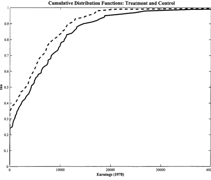
treatment effect (QTE). As originally defined by Lehmann (1974) and Doksum (1974), the QTE corresponds, for any fixed percentile, to the horizontal distance between two cumulative

Dok-sum (1974) and Lehmann (1974) implicitly argued that an observed individual would maintain

his rank in the distribution regardless of his treatment status. This paper will refer to this type

of assumption as a rank invariance assumption.

Rank invariance assumptions are strong assumptions as they require that the relative value

(rank) of the potential outcome for a given individual would be the same under treatment as

under non-treatment. There are two ways to deal with cases in which rank invariance is an

unreasonable assumption. The first one is due to Heckman, Smith, and Clements (1997), who

suggested computing bounds for the QTE, allowing for several possibilities of re-orderings of

the ranks. According to them, the outcome for the same individual may differ from one

distri-bution to another based on how observable and unobservable attributes impact each one of the

potential outcomes. However, while the effect of observable characteristics can be measured,

unobservable characteristics can interact with treatment status in many unknown ways, leaving

open the possibility of a sharp reordering of ranks. Bounds for the QTE that capture these

altematives were proposed by Heckman, Smith and Clements (1997).

The second approach to dealing with failures of the rank invariance assumption argues that

even without this assumption, one can still have a meaningful parameter for policy purposes.

Consider the case in which all the policy-maker is interested is in learning about the marginal

distributions of the potential outcomes. A good way to summarize interesting aspects of these

distributions is by computing their quantiles. In this case, quantile treatment effects can be

defined as simple differences between quantiles ofthe marginal distributions ofpotential

out-comes. As an example, suppose that one is interested in the difference in medians between two

distributions, and not in the effects of treatment on a typical individual. In such a setting it is

not necessary to have any knowledge about the joint distribution of outcomes for the treated

and control groups, so the rank invariance assumption could be dropped. Note, however, that

if rank invariance holds, then the simple differences in quantiles tum out to be the quantiles of the treatment.1

1 Note that there is no similar problem in estimation ofthe average treatment effect, as differences in means

This definition of quantile treatment effects, together with the selection on observables

approach, allows identification of various QTE parameters that differ by the subpopulation they

refer to. Following the approach ofHeckman and Robb (1986) and Hirano, Imbens and Ridder

(2002), who suggest several parameters of interest for the mean case, two QTE parameters

will be the object of study in this paper. They are labeled the quantile treatment e.ffect and

the quantile treatment e.ffect on the treated, the former being the QTE parameter for the whole

population under consideration and the latter the parameter for those individuaIs subject to

treatment. Defining T as the indicator variable of treatment, these parameters can be expressed

as:

Quantile Treatment Effect: .ó.t = ql,t - qO,t,

where qj,t is such that

Pr[Y(j)

S q]

=

't, j

=

0, 1.

Quantile Treatment Effect on the Treated: .ó.tIT=1 = ql,tIT=1 - qO,tIT=b

where qj,tIT=1 is such

thatPr[Y(j)

S qJ T

=

1]

=

't, j

=

0, 1.

The role that the observable covariates play in identification ofboth ATE and QTE is made

clearer in the QTE case. This is because, as stated earlier, the computation of quantile

treat-ment effects does not use the conditional quantiles. Computation of conditional quantiles is

unnecessary since the quantiles ofthe marginal distributions ofthe potential outcomes are the

object of interest and the mean of the quantile is not the quantile of the mean. Hence, for QTE,

the covariates serve only to remove the selection bias.

Quantile treatment effects are also useful in describing the center of the distribution of the

treatment. In particular the median treatment e.ffect (MTE), the QTE for the fifty percentile,

is a central measure of the treatment effect, like ATE. However, MTE has an additional and

desirable feature not present in ATE: its corresponding estimator is robust to the presence of

data outliers.

Despite the relevance of QTE, the program evaluation literature on this topic is not as

vast as that of its main competitor, ATE. Traditionally, expectations have received more atten-tion in the literature than quantiles. Pioneer papers on quantile estimaatten-tion, such as those by Koenker and Bassett (1978) and, in an instrumental variables setting, by Amemiya (1982) and Powell (1983) have helped to bridge this gap. In the treatment effects literature, some recent contributions have also been made to the study of the distributional effects of the treatment. Among them, Abadie, Angrist and Imbens (2002), and Chernozhukov and Hansen (2001) have proposed instrumental variables versions of the QTE. Imbens and Rubin (1997) and Abadie (2002) proposed methods to estimate some distributional features for a subset of the treated units, again in an instrumental variables setting. Distributional effects have also been stud-ied empirically, as in the papers of Freeman (1980), Card (1996), and DiNardo, Fortin and Lemieux (1996).

In this paper three different semiparametric ways of estimating each QTE parameter are presented. Each one corresponds to a particular way that the parameter can be identified from the observable data. These three ways will differ by the number and by the sort offunctionals of the observed data involved in estimating the parameter. I focus my attention on the estimation technique that requires estimation of only the propensity score. This estimator is the QTE analogue ofthe ATE estimator proposed by Hirano, Imbens, and Ridder (2002), and involves reweighting observations by the inverse of the propensity score. The estimator will be equal to the difference between two quantiles, which can be expressed as the solution to minimization problems, where the minimand, a sum of check functions, is a convex empirical processo Using the empirical process literature consistency and asymptotic normality results are derived. As the estimator has asymptotic variance equal to the semiparametric efficiency bound (which I compute using the techniques suggested in Newey (1990) and Bickel, Klassen, Ritov, and Wellner (1993», this is an efficient estimator for the QTE parameters.

The remainder of this paper is divided as follows. The next section presents a simple model of quantile treatment effects. In the third section I demonstrate how the identification

assumptions alIow expressing the parameters of interest as functionals of the observed data.

Semiparametric efficiency bounds for QTE parameters are presented in Section 4, while

sec-tion 5 presents the three estimasec-tion techniques (mensec-tioned above) and large sample properties.

Section 6 presents an empirical application for the estimator. Section 7 concludes.

2 A

SIMPLE MODEL OF QUANTILE TREATMENT EFFECTS

I start by assuming that there is an available random sample of N individuaIs (units). For each

unit i, let

Xi

be a random vector of observed covariates with compact support X C ~r. Define

Yi( 1) as the potential outcome for individual i under treatment, and Yi(O) the potential outcome

for the same individual without the treatment. Let the treatment assignment be defined as

h

which equals one if individual i is exposed to treatment and equals zero otherwise. As we

only observe each unit at one treatment status, we say that the unobserved outcome is the

counterfactual outcome. Thus, the observed outcome can be expressed as:

Vi (1)

To motivate, consider Yi as the observed earnings of individual i in a model of the impact

of a job training program on worker earnings. In this example,

Ti

is the indicator for the receipt

of training.

Potential outcomes depend on both observed and unobserved individual characteristics. For

each individual i, let cI,i and cO,i be functions, under the treatment and the control respectively, of vectors of unobservable attributes. In a job training program model for example, earnings

of each individual are a function of their pre-program observable characteristics, such as past

earnings, employment status, education, age, job experience, gender, and union status; they

are also a function of unobservable attributes, such as ability, motivation and some possible

Specifying the impact of X and (t], to) on the potential outcomes:

Yi(

1)

=

G]

(Xi,

El,i)

Yi(O)

=

Go(Xi,Eo,i)

(2)

(3)

I assume se1f-selection into treatment: individuaIs can decide whether or not to be treated.

When an individual i faces the decision whether or not to join the job training program, he

will weigh the gains and costs to him of both situations. Assume that an individual i predicts

his expected eamings (given his vector Xi) and his costs for each of the altematives. In other

words, the individual i chooses the state that yields the largest expected utility:

where u(·) is utility function, C] (., .) and

Co(·, .)

are some costs associated respective1y with

joining the training program and not joining it, and

lli

is a vector of variables that is unobserved

to the econometrician but not to the individual. AIso,

lli

is assumed to be independent of

(EI,i,tO,a. The effect of

lli

on the individual 's utility will depend on whether or not he enters the job programo For example,

lli

might be a reservation wage that enters as an argument

to a foregone eamings function. Individual i will then choose to take part in the program if

E[u(Y(

1))

IXi, lli]-

C]

(Xi,

lli)

~

E[u(Y(O))

IXi, lld -

Co

(Xi,

lli).

That is:2

T

=

n{E[u(Y(l)) -u(Y(O))

IXi,lld -:-

(Cl

(Xi,

lli)

-Co(Xi,lli))

~ O} (5)

Note how this model fits into the Roy model (1951) of income distribution.3 In the Roy model, an individual chooses the greater of the potential eamings given by two different

occu-pations. Here, the choice is based on the individual's expected eamings and on some individual

2The indicator function n{A} is equal to one if Ais true and zero otherwise.

3 See also Heckman and Honore (1990).

cost. Thus, after controlling for Xi, the choice of getting treatment will be independent ofthe

individual potential earnings, whiCh depends only on Xi and (f!,i,fO,i). That will hold as long

as lli and (fl,i,fO,i) are independent and the functional form of potential earnings is the one

described in Equations (2) and (3). The independence result can be written as:

(Yi(

1),

Y;(O))

is jointly independent of

1i

givenXj Vi (6)

Equation (6) is the the unconfoundedness asswnption labeled by Rubin (1977) . This

as-sumption was derived here as a result, but we needed to put some structure on the form of

the potential outcomes and on the form of the decision rule. We also needed to put stochastic

restrictions on the unobserved variables. Note however, that unless there is a gain in insight to

writing the model with the structure presented in Equations (2)-(5), Equation (6) could actually

have been our starting point.

I will maintain the structure of the above model for now. In this model, a rank invariance

asswnption can be obtained by imposing two additional requirements:

(i) Vx E X, GI (x, .) and Go(x,·) are either (a) strictly increasing functions or (b) strictly

de-creasing functions;

(ii)

Vi,

fl,i and fO,i are perfectly positively correlated.

These two asswnptions ensure that people do not change their position in the earnings ranks

in each one ofthe possible two states. These are strong asswnptions, in particularpart (ii). This

is the case when skills that are useful in one regime may not be as useful in another regime. 4

However, note that if these two extra requirements hold, then for every individual i such

that

Pr[Y;(I)

~ ql,'t], it must be the case that

Pr[Yi(O)

~ qO,'t].5 Therefore, calculations ofthe

difference ql,'t - qO,'t for all 't in the interval [0,1] yield the distribution ofthe treatment effects.

4In terms ofthe Roy model (1951), in a world with only two occupations, hunting and fishing, that assumption implies that the most able hunters are also the most able fishermen.

5The same would be true for the quantiles of the distribution of potential outcomes given T

=

1, that is, if

As rank invariance is in many cases a too strong assumption, I also motivate the interest in the differences in quantiles in a different way. Assume that there is a social welfare function, V, such that V depends on the individual utility functions. For simplicity, assume that each individual utility depends on his earnings only. Therefore, we can write V as a function of the eamings distribution of the whole population. In order to simplify the argument, imagine that there are two possible scenarios: we either treat everyone or treat no one.6 Under the first scenario, the distribution of earnings is then equal to distribution of Y( 1), which has the cu-mulative distribution function FI; while in the second scenario, the earnings distribution equals that of Y( O), whose cumulative distribution function is Fo. Ignoring social choice problems, as-sume that the policy-maker has to choose between these two distributions in order to maximize the social welfare function:

V*

=

maxV(F)

Fl,Fo (7)

In order to compare V(FI) with V(Fo) the policy-maker will need to calculate approximate distributions ofthe potential earnings, FI and Fo, and a good way to summarize a distribution is to compute its quantiles. If we compute a sufficient number of quantiles, we will end up having a discretized approximation of the distribution.

Consider then that each distribution is approximated by the calculation of a number P of quantiles. When P is equal to 100, we say that each quantile corresponds to a percentile. Doing that for both distributions, we have:

(8)

(9)

6 Altematives, as discussed in Manski (1997), include allowing individuais to choose their treatrnent status or assigning them to treatment based on observed characteristics.

The policy maker chooses between treatment and no treatment according to whether VI is

greater than Vo.

Say that both VI and Vo are linear in the quantiles, that is, say that:

VI = V(ql l,qI2, ... ,qll)

'P']5 ,

P

=

~al,fql,f

J=I

(10)

(11)

where aj,f and ao,f'

U

=

1, ... ,P) are parameters ofthe social welfare function.

Consider the case where for each 't E {~,~, ... ,1}, al,'t

=

ao,'t = a't. This is a fairly intuitive

case: The weights on the social welfare function are the same whether or not the treatment is

implemented. In this case, the decision to run a job training program would be consistent with

the following inequality:

(12)

Equation (12) motivates the difference in quantiles as the main object of interest for the

policy-maker. The decision to continue running the program depends crucially on the quantile

treatment effects for all the quantiles of interest, that is, for alI 't such that a't

::f.

0.1

A particular case ofEquation (12) would be when a't

=

O for all 't but for one 't'. This is the case, for example, when all the policy-maker is interested in is whether the training increases

the earnings of those at the lower tail of the distribution.

Other types of social welfare functions would lead to the calculation of other treatment

effect parameters. For example, say that V1

=

ql,O.25 and that Vo

=

QQO,O.25. This is the case in

QI,O.75 0,0.75

which the policy-maker aims to run ajob training program that decreases eamings inequality

measured in a particular way. In this example, if V_{1 -} Vo ~ 0, then the program reduces the gap

between quartiles (.75 and .25), that is, reduces earnings inequality.

3

IDENTIFICATION OF QUANTILE TREATMENT EFFECTS

PA-RAMETERS

As potential outcomes are only partially observed, in order to identify from the observed data

both L1, and ~ I T = 1, the quantile treatment effects and the quantile treatment effects on the treated, we need an identification restriction. Instead of writing that restriction in terms of

unobserved components (as in the previous section), I will start from a more general setting, in

which we do not need to know the functional form ofthe potential outcomes. Let the propensity

score, Pr[T = llX

=

x], be written as p(x), and its expectation, E [P(X)], be written as p. Thus, the identification assumption used here, following Rosenbaum and Rubin (1983), is:

ASSUMPTION 1 (Strong Ignorability - Rosenbaum and Rubin (1983)): For almost all values ofX:

(i) Unconfoundedness: (Y(I),Y(O)) isjointlyindependentfrom T givenX;

(ü) Common Support: c

<

p(x)

<

1 - c, for some c

>

°

Although it is a strong assumption, many studies of the effect of treatments or programs

make an assumption similar to that of part

(i)

of Assumption 1 as, for example, Heckman,

Ichimura, Smith, and Todd (1998) and Dehejia and Wahba (1999). Altematives to this

as-sumption are the using instrumental variables (the selection on unobservables approach), and

calculating bounds for the parameter of interest, as proposed by Manski (1997).8 Part (ü) states 8For review and comparison of approaches see, for instance, Angrist and Krueger (1999) and Heckman, LaLonde and Smith (2000).

that for almost alI values of X both treatment assignment leveIs have a positive probability of

occurring.

Now consider that each one of the four types of quantiles defined previously, ql;r, qO;r,

ql,'tl T=], and qO,'t1 T=l do exist and are uniquely deterrnined or, in other words, the distribu-tion funcdistribu-tions of the potential outcomes are continuous and not fiat at the t-percentile. These

conditions appear in the folIowing asumption:

ASSUMPTION 2 (Existence and Uniqueness ofQuantiles): For j

=

0, 1, YO) is a continuous random variable with support in ]R. such that for t E [0,1]:

(i) Existence: ~,j = {q E]R.I t = Pr[Y(j) ~ q]} and Q..,jIT=l = {q E]R.I t=Pr[Y(j) ~

ql T

=

1]} are non-empty.

(ii)Uniqueness: Let Fj(q)

=

Pr[Y(j) ~ q] and FjlT=l (q)

=

Pr[Y(j) ~

ql T

=

1].

'h

a~(q)1

+ ( )

°

daFm=l(q)1

f

(

)

°

r.

en q _ . =Jj qj,'t

>

an dq _

=

jlT=l qj,'tIT=l

>

q-q},t q-qj,tIT=l

Under Assumptions 1 and 2 both the overalI quantile treatment effect and the quantile

treatment effect on the treated become estimable from the data on (Y, T,X). To show this, I

first prove that the quantiles of the potential outcome distributions can be written as implicit

functions ofthe observed data:

LEMMA 1 (Identification ofQuantiles): Under Assumptions 1 and 2, thefollowingequalities hold:

ql,'t :

(Q1c)

= E[Pr[Y ~

ql,'tIX,

T

=

1]]

= [E[T n{Y

~

ql,dIXJ]

E p(X)

=

E[Tn{y~ql,'t}]

Proof: See Appendix I

Lemma 1 shows that there are multiple ways of expressing each quantile of the potential outcome distributions in terms ofthe observed data (Y, T,X).9 In fact, the lemma shows that there are at least three ways of identifying the quantiles using the observed data (Y, T,X). These are divided into three groups denoted by A, B and C (which are the indices for each expres-sion in Lemma 1). Each group will differ according to the number and type of conditional expectations to be taken inside the expectation symbol.

In the first identification group, indexed by A, the computation of a conditional probability function in the first step is required. This function is the probability of Y being less than or equal to q given that X

=

x and T

=

1. Taking the expectation over alI x E X for the treated

subset (T

=

1) yields the desired result: ql,t will be the quantity that sets the expected value equal to 'to

The equation indexed by B also requires computation of a conditional expectation in the first step. However, as this conditional expectation function is not restricted to the subset oftreated units, one needs to divide by the probability of being treated given X

=

x (the "propensity score"). Notice then, that the first step involves two conditional expectations computations. This is the price paid for not restricting computation to the subset of treated units. Also, as in expression A, in expression B ql,t wilI be the quantity that sets the expected value ofthe ratio of conditional functions equal to 'to

Finally, expression C is the simplest of the three. The first step requires computation of just one conditional expectation function, namely, the propensity score. Notice, that ex-pression A also requires just one conditional expectation computation in the first step. The main difference lies in the role that the quantile q plays. In A one first has to compute

KI (x;

q)

=

E[n{Y::; q}IX

= x,

T

= 1]. This function does not simply depend on (y,t,x), be-9 An analogous result for qO,t would follow from the same lines ofLemma 1. For example, for the group C we would have t - E [(I-T)I{y<QO,t}]

- l-p(X) .

cause the quantile q enters as an argument, complicating computation.10 This is different for expression C. In C, the p-score computation does not involve q; in fact, it does not involve

the random variable Y nor any functional of its distribution. Finally, to get

ql,'t,

one needs to

proceed as in the other steps and compute an unconditional expectation.

As Lemma 1 does not directly yield a way to identify the quantiles ofthe potential outcomes

for the actual treated units, it is necessary to postulate another set ofresults for that special case:

LEMMA 2 (Identification of Quantiles for the Treated): Under Assumptions 1 and 2, the

following two sets of equalities hold:

(QT1B)

(QT1c)

(QTOB)

(QTOc)

Proof: See Appendix I

= E[p(x)pr[y:::;ql;IT=lIX,T=

ll]

= E [E[T n{Y:::;

!l,'tIT=l}IXl]

E [T n{Y:::;

;l,'tIT=d]

E [p(x)pr[Y:::; qO;IT=lIX, T

=

Ol]

E

[(1

!;~l))pE[(l-

T)n{Y:::; qO,'tIT=dIXl]

= E

[(1

!;~l))p

(1-

T)n{Y:::; qO,'tIT=l}]

In the proof in the Appendix I, one can see that Assumption 1 plays no role in the

iden-tification of ql;tl T=l· Heckman, Ichimura, and Todd (1997) have stressed such result when

looking for identification conditions for the average treatment effects on the treated.

Identification of the quantile treatment effect parameters parameters is a straightforward

consequence of Lemmas 1 and 2, as stated in the next corolIary.

COROLLARY 1 (Identification of quantile treatment effect parameters): Under Assumptions 1 and 2, the quantile treatment effect, ~'t, and the quantile treatment effect on the treated,

~IT=l' are identifiedfrom data on (1', T,X).

Proof: Note that from Lemmas 1 and 2 the four parameters ql,'t, qo,'t, ql,'tIT=l> and qO,'tIT=l

are functionals of the joint distribution of (Y, T,X). As ~'t equals the difference between ql,'t

and qO,'t; and ~IT=l equals the difference between ql,'tIT=l and qO,'tIT=l, ~'t and ~IT=lare

also functionals ofthe joint distribution of (Y, T,X). Therefore, ~'t and ~IT=b are identified

from data on (Y, T,X). O

For ~IT=b the method given by group A requires the computation ofthe p-score in

ad-dition to the computation of one conad-ditional expectation given T

=

1 and X for (QT1A), and another conditional expectation given T = O andX for (QTOA). The method in group B requires computing one conditional expectation givenX for (QT1B) and computing another conditional

expectation as welI as the p-score for (QTOB). FinalIy, for group C alI that it is required is the

p-score computation for (QTOc). Notice that the expectation ofthe p-score, p, is required for

alI three groups.

A comparison between Lemmas 1 and 2 reveals the presence of an interesting asymmetry

in the former but not in the latter. Using procedures B and C, the computation of ql,'tIT=l

requires fewer first step calculations of conditional functions than the computation of q O,'t I T= 1.

This difference does not hold for ql,'t versus qO,'t, since the computation ofthese are symmetric

and both computations involve the same number and sort offunctionals.

From an estimation point of view the classification of these three groups of methods is

relevant not only for the QTE, but for mean-based measures, such as the ATE, as well. Using

sample analogues, Hahn (1998) has suggested estimation of the ATE based on an identifying

approach similar to that described by B. Dehejia and Wahba (1999) proposed (among other

techniques) estimating the average treatment effect on the treated by reweighing the control

sample using the estimated p-score; this is analogous to the identification set C. Hirano,lmbens

and Ridder (2002), going into more detail, have also focused on the estimation of ATE using

the analogue of the set C for identification.

Estimation of the quantile treatment effect on the treatment based on the set C of identifying

assumptions has been implicit in the applied literature. DiNardo, Fortin, and Lemieux (1996)

proposed estimation of the counterfactual density of outcomes for the control group using a

method similar to (QTOc). They argue in a footnote that, once the counterfactual density

is estimated, it is possible to recover the counterfactual quantiles and therefore the difference

between the quantiles ofthe treated group and the counterfactual quantiles ofthe control group.

However, as is made clear by expression (QTOc), there is no need to first compute densities if

the ultimate goal is the estimation of quantiles.

In Section 5 of this paper I present the estimation counterparts of alI three sets of equations

for both the overalI quantile treatment effect and the quantile treatment effect on the treated.

4

SEMIPARAMETRIC EFFICIENCY BOUNDS

As Lemmas 1 and 2 suggest, estimation of quantile treatment effects can be attempted using

a two-step procedure, where the first step is a non-parametric estimation of a conditional

ex-pectation function. The preliminary step must be non-parametric since the joint distribution

of (Y(O), Y(I)) is not parametricalIy specified. Semiparametric estimation for the ATE can be

found in Hahn (1998), Heckman, Ichimura, Smith, and Todd (1998) and Hirano, Imbens and

A semiparametric analog of the Cramer-Rao lower bound was first introduced by Stein

(1956) and further developed by Bickel, KIassen, Ritov, and Wellner (1993). The

semipara-metric efficiency bound concept was popularized in the econosemipara-metric literature by a review

article by Newey (1990). In general terms, the bound corresponds to the largest variance over

all possible regular parametric specifications of the nonparametric component of the mode!.

Such bound is indeed a (not necessarily achievable) lower bound for the asymptotic variance

of distribution-free, root-N consistent estimators.

More formally, consider a finite-dimensional parameter

ç

from some general statistical

mode!. Say that this model contains a submodel that can be parameterized by a finite-dimensional

parameter

8.

Thus, for this submodel we write

Ç(8).

Ifthis parameter is differentiable in the

sense described by Bickel, KJassen, Ritov, and Wellner (1993), then its derivative with respect

to 8 can be written as E['Vs~], where 'V is the influence function of

ç

and se is the score of that submode!. The semiparametric efficiency bound

Vç

will be equa1 to E [%'Ve] , where 'Ve is

equal to E['Vs'e](E[ses~])-l Se, the "projection" onto the space spanned by all scores.

Hahn (1998) uses the setup described above to compute the semiparametric efficiency

bounds for both the average treatment effect, ~, and the average treatment effect on the treated,

y. For the quantile treatment effects setting, I also compute bounds for two parameters, namely,

~t and ~IT=l. With Assumptions 1 and 2, the semiparametric efficiency bounds for ~t and

~IT=l can be calculated:

THEOREM 1 : (Boundsfor ~t and ~I T=l): Under Assumptions 1 and 2, the semiparametric efficiency boundsfor ~t and ~IT=l are respectively equal to:

_ [V[gl,Llt(Y)IX, T =

1]

V[gO,Llt(Y)IX, T =

O]

VLlt -E p(X)

+

1 _ p(X)

+

(E[gl,Llt(Y) IX, T = _{1]-E[gO,Llt(Y)IX, T}

=

0])2]

(13)

and

wherefor j

=

0,1:

(15)

and

(16)

Proof: See Appendix I

Note that the bounds VÓt and V ~IT=I are similar to the bounds computed by Hahn (1998)

for the mean case. For

B

and

r

the bounds, as computed by Hahn (1998), are respectively: 11

[

V[YIX,T=

1]

V[YIX,T=O]

2]

V~=E

p(X)

+

l-p(X)

+((E[YIX,T=I]-BI)-(E[YIX,T=O]-Bo))

and

v;

=E [P(X)V[Y IX, T

=

1]

+

",-p(,-X"-7?...,.-'V[,--Y-,-IX..,.-'

T--:-:=~O]

Y

p2

p2(I-p(X))

p(X)((E[Y IX, T

=

1] -

rI) -

(E[Y IX, T

=

0]-ro))2]

+

2 .

P

There are two reasons for the similarity between the semiparametric efficiency bounds of

the QTE and the ATE parameters. First, both the QTE and the ATE are parameters from the

same statistical model and, therefore, can be expressed as functionals of the same distribution of the data. But this is not enough for the similarity. In fact, the second reason is the im-portant one: both the QTE and the ATE are written as differences in expectations of random variables (implicitly for the QTE case) over the same density. This can be seen in the following equations: 12

d"C = arg zeroqE[ll{Y( I) ::; q} -

1]-

arg zeroqE[ll{Y(O) ::; q} -

1]

(17)

and

~

=

E[Y(I)]-E[Y(O)] (18)

Note that what ultimately determines the difference in the bounds is the distinction between the random variables gj,D., (Y(j)) and Y(j), respectively the influence functions of qj,"C and of

~ j when Y is independent of X.

The role of the propensity score in efficient estimation of ATE has received a great deal of attention in the recent literature. Examples include Heckman, Ichimura, Smith and Todd (1998), Hahn (1998) and Hirano, Imbens, and Ridder (2002). The latter provide intuition for Hahn's result that knowing the true propensity score does not lead to efficient estimation ofthe ATE. For the QTE parameters the same results apply since both cases share the same statistical model, and thus the propensity score plays the same role. Because ofthis similarity, this result will not be further explored in this paper.

5

EFFICIENT ESTIMATION

Once we know which parameters we want to estimate and we know the minimum attainable asymptotic variance of any semiparametric estimator, we can propose candidates for

estima-12Note that this argument could be very well be applied to the comparison between the "on the treated" param-eters, ~I T= I and y.

[20]

BIBLIOTECA

MARIO HENRIQUE. SIMOrtSEft

tion. In this section I use the sample analogy principIe 13 to motivate the appropriateness of the usage of estimators of ~'t and ~I T=1 that are in fact solutions to minimization problems.

Restricting then attention to one of the estimators, I present its large sample properties and

also show that the asymptotic variance of the proposed estimator achieves the semiparametric

efficiency bound.

5.1

MINIMIZATION ApPROACH

According to Lemmas 1 and 2 there are at least three ways of identifying the quantiles of the

potential outcome distribution. From the sets A, B and C of identification expressions, it is

pos-sible to derive three different estimators for both the ~'t and ~

I

T=1 parameters. The estimators

will differ among themselves by the number and type of conditional expectations functions to

be non-parametrically estimated in a first step. As a piece of notation, let the first step

esti-mators of functionals of (Y, T, X) be denoted by a "hat" on it. For example, the nonparametric

estimator of the p-score will be p(

x).

In order to simplify the following argument, let me focus

only on the three estimators of ~'t, which will be, for E E {A,B,C}:

ÁE ~ ~

"'4 =

'11,'t - '10,'t

(19)

where for j = 0, 1:

N

tJ7,'t

=

argmin

L

Ôl7,iP't(Ji -

q)

q

i=1

(20)

and where the check function

P't(')

evaluated at

}f -

q is:

P't(}f -

q) =

(}f -

q)('t -

n{}f -

q S;

O})

The previous definitions of the estimators rely on the fact that sample quantiles can be found by minimizing a sum of check functions.14 In our particular case, we have a weighted

sum of check functions, which reflects the fact that as we do not observe the two potential outcomes for the same unit, a rescaling over the observed units is necessary. AIso note that for the definition to be complete, I need to determine what the weights

roJ,i

are.

Once again for simplification, let us focus on the estimation technique C and concentrate on the sample quantile ofthe Y(I)'s distribution,

qf't.

This sample quantile is defined as the minimizer of a weighted sum, where the weight of each unit is given by:

(21)

To get some intuition on why

qf't

is actually consistent for ql,'t, notice that an approximate first derivative ofEquation (20) using the weight defined in Equation (21) and evaluated at

qf't

is equal to:

~

f

L(n{}f

~

qf,'t}

--r)

N i=1 p(~)

(22)

As

qf't

_, is the minimizer ofthe convex function expressed in Equation (20) using the weight defined in Equation (21), Equation (22) will converge in probability to zero as N increases. Therefore, Equation (22) is the sample analog ofthe identifying expression (Qf) in Lemma l. Note that this intuition works also for the other two estimators of ql,'t:

tl1,'t

and

qf,'t"

For a more detailed discussion on how to find weights for the cases A and B, see the Appendix 11.

The same line of reasoning could have been applied to estimation of Li'tl T=I. Each esti-mator will be defined as the difference between the solutions of two minimizations of sums of weighted check functions. For E E {A,B, C}:

14See, for instance, Koenker and Bassett (1978).

In particular, for the estimation procedure indexed by C, the weights are equal to:

and (24)

This result will be used later in the paper. Before that, however, let us turn our attention on the computation of the weights used in this subsection. In particular, let us concentrate on the

calculation of

rof,i.

5.2

FEASIBLE ESTIMATION

For the remainder of the paper, I shall restrict the discussion to estimators that use the set C of

identifying equations. As argued before, these are the simplest estimators. I will also focus on

qf.

t only since extensions for

q~

t and for

~~I

T = 1 follow immediately.

The estimator qf,t is a two-step .estimator. In the fust step, we estimate the p-score

non-parametrically. In the second stage, we minimize:

(25)

Equation (25) is a weighted sum of check functions. Following Koenker and Bassett (1978),

I find sample quantiles as minirnizers of sums of check functions. However, I have a weighted

sum of check function, as the weights are the way used here to correct for the selection.

My specific methods were as follows: To estimate the p-score, I used a logistic power

series approximation, i.e., the log odds ratio of the p-score was approximated by a series of

functions.15 These functions were chosen to be polynomials of x and the coefficients corre-sponding to those functions were estimated by maximum likelihood.

Start by defining

HK(X)

=

[HK,j(X)]

(j

= 1, ...

,K),

a vector of length

K

of polynomial

functions of x E X satisfying the following properties:

(i) HK: X

--+

~K;

(ii)(Constant included)

HK,I (x)

= 1

Ifwe wantHK(x) to include polynomials ofx up to the order n, then it is sufficient to choose

K such that K ~

(n

+

1

y.

In what follows, I will assume that K is a function of the sample size

N and grows without bounds as N grows without bounds, that is, K

=

K(N)

--+

00 as N

--+

00.

Next, the propensity score is estimated. Let

jJ(x)

be:

jJ(x)

=

L(HK(X)'it)

(26)

where

L:

IR

--+

~,

L(z)

= (1

+

exp( -z))-

1 and

it

=

argm:x

~ ~ {1iln(L(HK(~)'1t))

+

(l-1i)ln(l-L(HK(~)'1t))}

(27)

Thus, after estimating the p-score, I minimize GN(

q, jJ)

with respect to

q,

obtaining

tiL.

_,

5.3

LARGE SAMPLE PROPERTIES

In this subsection I will prove that

qY,'t

is (i) root-N consistent for ql,'t; (U) asyrnptotically

normal; and (Ui) has asymptotic variance equal to the expected square of the efficient infiuence

function of ql,'t. 16

This subsection is divided into several parts, each one corresponds to a step in the proof:

16Thus, as ÓT

=

ql,T - qO,T and as it can be shown by analogy that qÕ,T equally satisfies the properties (i), (ii) and a properIy modified version of (iii), the effi.cient infiuence function of óT will be equal to the difference between the effi.cient infiuence function of ql,T and qO,T.

1. I state the assumptions and the results derived in Hirano, 1mbens and Ridder (2002) for

the asymptotics properties ofthe non-parametric estimation ofthe p-score in the first step

by means of a power series approximation.

2. I use a tranformation from q to

t

= q - qI,"t and define

QN(t,p),

which is minimized by

~ ~C

t = qI,"t - qI,"t·

3. I use another transformation,

u

=

VNt,

and show that

N(QN(U/VN,p) - QN(u/VN))

is op(l) for fixed

u,

where

QN(u/VN),

which does not depend on

p(x),

is a quadratic

random function.

4. I show that ü, the argument that minimizes the random quadratic

NQN(U/VN),

is: (i)

Op(l); and (U) ü

~

N(O, VI), where VI is the semiparametric efficiency bound of ql,"t.

5. I show that the term ú

=

VNr

is just op(l) from ü, or written in terms of q, that ti?,"t is asymptotically equiva1ent to ilI,"t =

ü/

VN

+

qI,"t, which establishes the desired result.

5.3.1 ASYMPTOTIC PROPERTIES OF THE FIRST STEP

The suggested approach to estimating the p-score guarantees, under certain regularity

condi-tions, that

p(x),

the estimator ofthe p-score, is uniform1y consistent for the true

p(x).

To assure

that this holds, I make the following assumptions:

ASSUMPTION 3 (First Step):

(i) X is a compact subset of~ r;

(ii) the density ofX, f(x), satisfies

0<

infxEXf(x) :::; sUPxEXf(x)

<

00

(iii) p( x) is s-times continuously difJerentiable, where s

2':

7 r and r is the dimension of X; (iv) the order ofHK(X), K, is oftheform K

=

CN(J. where C is a constant and

a

E (4(~~I)'~)

Newey (1995, 1997) has established that for orthogonal polynomials HK(X) and compact

Ç(K) = sup IIHK(X)II ~ CK (28)

xEX

where C is a generic constant. Note then that because ofpart (iv) of Assumption 3

ç

will be a

function of N since K is assumed to be a function of N.

With part (ii) of Assumption 1 (Common Support) and Assumption 3 in hand we can invoke

some of the results derived by Hirano, 1mbens and Ridder (2002) in a format of a lemma:

LEMMA 3 (First Step): Under Assumptions 1 and 3 the following results hold:

(1)

sUPXEX

Ip(x) -

PK(X)

I

~ CÇ(K)K-sjr ~ cçl-sjr ~ CN(1-sjr)a. = 0(1); where:

and:

nK

=

argm;xE

{P(X) In(L(HK(X)'n))

+

(1- p(X)) In(l -L(HK(X)'n))};

(II)Ellit-nKI12

~

_Cçr:;)

~

_{CNa.-l = 0(1);}

(III) There is 8

>

O: limN-+ooPr[8

<

infxExp(X)

~

sUPXEXP(X)

<

1- 8] = l.

Proof: See Hirano, 1mbens and Ridder (2002).

(29)

(30)

Note the importance of result (III) in simplifying the whole process of estimating ql,'t by

qf,'t.

As

p(x)

is bounded inprobability from O and 1, there is no need to use a trimming function

in order to avoid dividing a number by zero.

5.3.2 CHANGE OF VARIABLES: t AND

QN

First notice that:

ti?,'t

= argmin

~

f

~(~.)

(Ji -q)(t - ll{Yi

~

q})

q i==1 P 1

1 N Ti [ ]

=

argmin

N

~ ~(~.)

(fi - q)(t - ll{Yi

~

q}) -

(Yi - ql,'t)(t -

ll{Ji

~

ql,'t})

q 1==1 P 1

1 N Ti [ ]

= argmin N ~ ~(~.)

(ll{Ji

~

ql,'t} - t)(q -

ql,'t)

+

(fi -

q)(ll{Ji ::; ql,'t} - ll{Ji ::; q})

q 1==1 P 1

Now, define:

t =

q-ql,'t

~ ~C

t

=

ql,'t - ql,'t

D(Ji)

=

ll{Ji ::; ql,'t} -

t

R(Ji, t)

=

(Ji - (ql,'t

+

t))(

ll{Ji ::; ql,'t} - ll{Ji ::; ql,'t

+

t})

A(Ji,t)

=

D(Yi)t+R(Ji,t)

(

~)

1

~

Ti

(

)

QN

t,p

=

N ~ ~(X)A

Ji,t

1==1 P 1

(31)

(32)

(33)

(34)

(35)

(36)

(37)

A comment about some ofthe quantities above: The variable

D(Yi)

is the approximate first

derivative ofthe check function

P(Yi - q)

with respect to

q.

It is approximate in the sense that

p(

Ji - q)

is not differentiable for all

q,

as it involves indicator functions of whether

q

is less

than or equal to some values in the data.

R(Yi, q - ql,'t)

can be interpreted as the remainderterm

from a linear expansion about

ql,'t

that uses

D(Yi)

as an approximated derivative.

i

=

arg~in~

f

~(~o)

[(1I{Y;:::; ql;r}

-'t)t+

(Y;- (ql;r+ t ))(lI{Yi :::; ql,,:} -lI{Yi :::; ql;r+ t})]

1=IP I

=

argmin~

f

~(I;)

[D(Y;)t+R(Yi,t)]

t Ni=IP

Xi

1 N r; = argmin

N

L

~(Xl

o)A(y;,t)

t i=IP I

=

argminQN(t,p)

t

5.3.3 A QUADRATIC ApPROXIMATlON TO THE OBJECTlVE FUNCTION

(38)

(39)

(40)

(41)

I begin by defining some useful expressions: First, consider the function

QN(t),

which will be

shown to be a quadratic approximation to

QN(t,p),

which, however, does not depend on the

first step p(X):

Now, define:

(43)

and

u=

VNt

(44)

The next lemma shows that NêN(U/VN) goes to zero in probability for each

u,

which

means that the objective function is asymptotically equivalent to a quadratic random function.

Before stating the lemma, let me first assume that the next regularity condition holds:

ASSUMPTION 4 (Lipschitz condition): For j = O, 1 and every t, the conditional density of

Y(j) given X = x, Jj(·Jx), satisfies thefollowing inequality, where E[M(X)]

<

00, and À> O:

(45)

LEMMA 4 (Bounding the difJerences in the Objective Functions): Under Assumptions }, 2,

3 and 4,for each u:

(46)

Proof: See Appendix I

5.3.4 ASYMPTOTIC PROPERTIES OF ii

We have used Assumption 2 previously both for identification of quantiles of the potential

outcomes and for an appropriate definition of the efficiency bounds. The same assumption is

plays another role in this subsection; it guarantees that

a,

the argument that minimizes N

QN(

u)

is unique. From Equation (42) we have:

(47)

= _

1

f

(TiD(Y;) -E[D(Y)IXz',T= 1JTi-p(Xz-))

(48)

v'N

fI

(ql;r) i=1

p(J4)

p(Xi)

1 N

=

hrN

L

'V1,i (50)

VIV 1=1

where the function gl ,t1

t was defined by Equation (15) and:

Let me now write the main result of this subsection as a lemma:

LEMMA 5 (Asymptotic Properties oJíl): Let íl

=

argminuNQN(u/v'N). Then, under

As-sumptions 1, 2 and 3:

(i) íl

=

Op(l);

(ii) íl

Et

N(O,E['VL));

(iii) E['VI,J

=

VI, the semiparametric efficiency boundfor ql;r·

Proof: See Appendix I

5.3.5 NEARNESS OF ARGMINS

Defining

u

=

v'Nt, I show the desiredresult that

u-

íl

=

op( 1), which will implythat

..;N(qf

_, 1:-ql,1:) is (i) Op(l), (U) and asymptotical1y normal (Ui) and has an asymptotic variance that is

equal to the semiparametric efficiency bound for ql,'t. Before I do that, let me state and prove

an intermediate lemma.

We have already seen that Lemma 5 holds. To get results about íi and consequently about

qÍ,'t

I will use a result in Hjort and Pollard (1993) on the nearness of minimizers of convex

random functions.

I apply Hjort and Pollard's Lemma 2 directly to my case:

LEMMA 6 : (Nearness of Argmins (Hjort and Pollard (1993)) Under Assumptions 1, 2, 3

and 4 we have the following probabilistic bound on how far íi can be from

u:

For each Õ

>

O:

Moreover:

Proof: See Appendix I

Stating the final results:

(52)

(53)

T _HEOREM 2 _{: lf:1symptotlc ropertles oJ} /" . P . ,./.'C _Iql,v I L _{et ql,'t -}'c - _argInln. I .... N JL(i'i )( q N ":"i=1 p(Xi) i - q ' t

-ll{Yj::; q}) where

p(x)

is computed as described in subsection 5.2. Under Assumptions 1, 2, 3

and 4:

(i)

VN(qÍ,'t -

ql,'t)

=

Op(l)

(ii)

VN(qÍ,'t

-ql,'t)

=

JNL~I

\jfl,i+op(l)

I N D ( )

where

JN

Li=1

\jfl,i -+ N O, VI ;

Proof: Defining iÍl,"C =

u/ VN

+

ql,"C, by Lemma 6 we have:

vNlqf,t - 'lI,tl =lvN(qf,t -

ql,t) - VN(qf,t -

ql,t)1

:Slu-ul

=op( 1)

(54)

That is,

qf,t

is asymptotically equivalent to (JI,t and Theorem 2 follows immediately by Lemma 5. O

The same result obtained for ql,t could have been obtained analogously for qO,t. In

partic-ular, with the same set of assumptions used in Theorem 2, it is possible to derive an asymptotic

linear influence function for q5,t' "'0, which is analogous to "'I· In fact, "'O,i

=

12

;[k)

(gO,llt

(lí)

-E[gO,llt(Y) IXi , T

=

O])

+E[gO,llt(Y) IXi , T

=

O].

A consequence of Theorem 2 is that ~, which is equal to the difference between qf, t and

q5,t:

(i) will also be consistent, (ii) will have an asymptotically linear influence function and, (iii) will be asymptotically normal:

THEOREM 3 : (Asymptotic Properties 01 ~): Under Assumptions 1,2,3 and 4:

'c p

(i) 11'i - Ôt -+ O

(ii)

VN(~

- Ôt )

=

J;vIf:1

"'i+

O

p(1)

(iii)

VN(~

-

Ôt )

~

N(O, Vt )

where "'i

=

"'I,i - "'O,i and

V

=

E [V[gI,ót(Y)IX,T=I]

+

v[go,L'>t(Y)IX,T=O]

+

(E[g (Y)IX T

=

l]-E[go (Y)IX T

=

0])2]

llt p(X) l-p(X) I , l l t ' , l l t '

Proof: Omitted.

Theorem 3 shows that besides ~ being

root-N

consistent and asymptotically linear, it is

efficient, as it achieves the semiparametric lower bound for ôt .

Estimation ofthe quantile treatment effect on the treated, Ôtl T=I, will yield a similar result,

which could have been obtained using analogous steps to those used for the overall quantile treatment effect, .ó."C, to get results similar to Theorem 3.

6

EMPIRICAL ApPLICATION

In this section I consider one empirical application for the QTE estimators proposed in the previous sections. This application uses the job training program data set first analyzed by LaLonde (1986) and later by many others, including Heckman and Hotz (1989), Dehejia and Wahba (1999), Smith and Todd (2001) and Abadie and Imbens (2002).

The original data set from the "National Supported Work Program" (NSW) is well de-scribed in LaLonde (1986). The program was designed as an experiment as applicants were randomly assigned into treatment. The treatment was work experience in a wide range of pos-sible activities, like leaming to operating a restaurant or a child care center, for a period not exceeding twelve months. Eligible participants were targeted from recipients of AFDC, former addicts, former offenders and young school dropouts. The NSW data set consists of informa-tion on eamings and employment (outcome variables); whether treated or not; and background characteristics, such as education, ethnicity, age, and employment variables before treatment. LaLonde uses this experimental data set as a benchmark for comparisons with the case in which control samples come from non-experimental data sets, as for example, control samples based on Panel Study of Income Dynamics (PSID) and on Westat's Matched Current Popu-lation Survey-Social Security Administration File (CPS-SSA). I use on1y a subsample from the PSID, which corresponds the subsample termed "PSID-1"by Dehejia and Wahba (1999). Summary statistics for the two data sets are presented in Table 1. As this table reveals, the non-experimental control group is essentially different from the treated group, which leads us to tum the attention to the parameters of the treatment effect on the treated. In what follows here, the outcome variable is eamings in 1978.17 As in Dehejia and Wahba (1999) I consider

male workers only.

LaLonde finds that non-experimental control samples are poor substitutes for experimental data. Some reasons for those findings are described in the survey paper by Heckman, LaLonde and Smith (2000) and explored subsequently by Smith and Todd (2001). Three reasons that do not depend on the estimating procedures but on the data quality of the non-experimental data set are the following. A first reason relies on the fact that the non-experimental data set is not ofthe same type ofthe NSW, which implies that same variables are obtained from distinct questions and questionnaires. A second reason is the fact that comparisons groups obtained from surveys that do not cover only the original local labor market where the program took place should not be used to assess the impact of the program on that specific labor market. A third reason is that both data sets must have a sufficient number of relevant variables that explain the participation decision, which might not necessarily be the case for the NSW data set.

The choice ofthe estimation procedure also contributed for LaLonde's findings on the per-formance of comparisons using non-experimental samples. Dehejia and Wahba (1999) used the same data set as LaLonde (1986) and reached a different conclusion than LaLonde did. A first reason for the difference in conclusions come from the choice ofwhich pre-program vari-ables to include.18 _{Another important difference relies on the parametric nature ofLaLonde's}

analysis using non-experimental control groups. While LaLonde estimates parametric wage regressions for treatment and control groups which are intrinsically different from each other, Dehejia and Wahba use a more fiexible methodology. Their methods involve considering dif-ferentiallythe control units based on some closeness measure oftheir observable characteristics to characteristics ofthe treatment group.

In Dehejia and Wahba's estimation ofthe ATE on the treated, they estimate the propensity score in a first step using logistic regressions and propose several ways of using it to control 18Dehejia and Wahba included information on previous two years eamings, what reduced the treated sample in about 40%. See Dehejia and Wahba (1999) and Smith and Todd (2001).

for the selection problem. One of these methods, reweighing using the estimated p-score, uses

exactly the weights described by Equation (24),

CÔf,I"IT=1

and cô~iIT=I'

One data set Dehejia and Wahba use is a subset of 185 treated units and 2490 control

ob-servations from the PSID.19 Dehejia and Wahba estimate the p-score using logistic regression. The specification ofthe logit model is an issue in theirpaper, and it varies for each control

sam-pIe, because they are trying to find a specification that best "balances" each covariate between

treated and control groups. Next, they compute the average treatrnent effect on the treated,

which is equal to

2:7=1 (côf,il T=1 -

cô~iIT=I)r;·· For these specific treatrnent and control groups

they find an average treatment effect on the treated ofUS$ 1129.20 This is lower than the un-adjusted experimental treatment effect of $1749, but larger than the initial nurnbers LaLonde

cbmputed using the non-experimental data.21

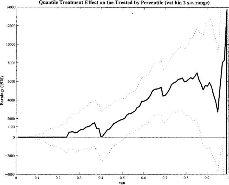
Using the same data, I analyze the treatrnent and control subsets to generate estimates ofthe

quantile treatrnent effect on the treated for each percentile. I also perforrn an "experimental"

QTE estimation, which is just the difference between the quantiles of the treated and the

ex-perimental controls, without any weighting. My results are presented in Table 2 and in Figures

I to 5.22 _{I find that using experimental controls, treatment effects tend to be more homogenous}

than in the observational setting. With a non-experimental control sample, treatrnent effects

seem to be above the median until almost the upper end of the distribution. At the extreme

upper quantiles, the very high earnings of the control sample induce a negative effect. Despite

the fact that the counterfactual c.d.f. ofthe control group introduces a heterogeneity in effects

not seen by using the experimental control, the difference between the two lies around zero, as

it is shown by Figure 5.

An important feature of the estimated counterfactual distribution is that there are some

19 As mentioned earlier this corresponds to the control sample labeIled by LaLonde (1986) and Dehejia and Wahba (1999) as PSID-I, as they constructed more than one control group based on PSID.

2°1 replicated their calculations using the same p-score specification and got a slightIy different number, $1120. 21 The unadjusted for covariates treatment effect was computed using the experimental control sample of size 260. It is a simple difference in means between treated and control groups.