ISSN 1678-992X
ABSTRACT: The aim of this study was to evaluate the performance of pedotransfer functions (PTFs) available in the literature to estimate soil bulk density (ρb) in different regions of Brazil, using different metrics. The predictive capacity of 25 PTFs was evaluated using the mean abso-lute error (MAE), mean error (ME), root mean squared error (RMSE), coefficient of determination (R2) and the regression error characteristic (REC) curve. The models performed differently when
comparing observed and estimated ρb values. In general, the PTFs showed a performance close to the mean value of the bulk density data, considered as the simplest possible estimation of an attribute and used as a parameter to compare the performance of existing models (null model). The models developed by Benites et al. (2007) (BEN-C) and by Manrique and Jones (1991) (M&J-B) presented the best results. The separation of data into two layers according to depth (0-10 cm and 10-30 cm) demonstrated better performance in the 10-30 cm layer. The REC curve allowed for a simple and visual evaluation of the PTFs.
Keywords REC curve, model evaluation, soil database, tropical soil
How accurate are pedotransfer functions for bulk density for Brazilian
Raquel Stucchi Boschi1*, Felipe Ferreira Bocca2, Maria Leonor Ribeiro Casimiro Lopes-Assad3, Eduardo Delgado Assad4
1University of São Paulo/ESALQ – Dept. of Soil Science, Av.
Pádua Dias, 11 – 13418- 900 – Piracicaba, SP – Brazil.
2University of Campinas/FEAGRI, Av. Cândido Rondon, 501 –
13083-875 – Campinas, SP – Brazil.
3Federal University of São Carlos/Center of Agricultural
Sciences, Rod. Anhanguera, km 174 – 13600-970 – Araras, SP – Brazil.
4Embrapa Agricultural Informatics, Av. André Tosello, 209 –
13083-886 – Campinas, SP – Brazil. *Corresponding author <[email protected]>
Edited by: Silvia del Carmen Imhoff
Received September 05, 2016 Accepted December 21, 2016
Introduction
Bulk density (ρb) is an important soil physical property known to affect soil water movement, root growth, seed germination and root density (Mouazen et al., 2003; Dexter, 2004). This property has received par-ticular attention due to its importance in weight-to-vol-ume conversions used to assess soil organic carbon (OC) stocks. Soil is known to contain the largest terrestrial carbon pool and can act as an important sink or source for atmospheric CO2.
Despite their importance, ρb databases are in short supply because direct measurements of undis-turbed samples are labor-intensive and time-consuming. Furthermore, ρb is highly variable in space and time (Al-letto and Coquet, 2009).
Pedotransfer functions (PTFs) (Bouma, 1989) have been widely used for estimating ρb using soil properties which are easier to measure and are available in most da-tabases. These PTFs have been developed from specific datasets using OC and texture data as input parameters (Curtis and Post, 1964; Alexander, 1980; Federer, 1983; Grigal et al., 1989; Huntington et al., 1989; Manrique and Jones, 1991; Bernoux et al., 1998; Tomasella and Hodnett, 1998; Kaur et al., 2002; Prévost, 2004; De Vos et al., 2005; Périé and Ouimet, 2008; Han et al., 2012; Al-Qinna and Jaber, 2013; Hong et al., 2013; Nanko et al., 2014). Benites et al. (2007) also used the sum of basic cations (SB) as an input parameter.
A number of studies have also tested the perfor-mance of available PTFs and observed that these func-tions are relatively inaccurate when applied to differ-ent environmdiffer-ents (Kaur et al., 2002; De Vos et al., 2005; Benites et al., 2007; Al-Qinna and Jaber, 2013; Nanko
soils?
et al., 2014). These studies assessed the performance of PTFs based on several error measures required for a re-liable evaluation. The root mean squared error (RMSE) and mean error (ME) are the most commonly used mea-sures (De Vos et al., 2005; Benites et al., 2007; Al-Qinna and Jaber, 2013; Nanko et al., 2014).
The aim of this study was to evaluate the predic-tive capability of PTFs available in the literature to es-timate soil ρb in different regions of Brazil, using dif-ferent metrics (mean absolute error (MAE), root mean squared error (RMSE), mean error (ME) and regression error characteristic (REC) curve).
Materials and Methods
Selected pedotransfer functions (PTFs)
We evaluated 25 PTFs available in the literature. The PTFs selected, R2 values and the size of the data
set used to generate the PTFs are shown in Table 1. PTF equations were adjusted to the same units for bet-ter comparison. The details about land use, location, ρb range, and the method used to determine the ρb, which was extracted from the original papers, are presented in Table 2.
Data set
The original data set used to evaluate the perfor-mance of the 25 PTFs consisted of 222 soil profiles (888 soil layers) distributed in different biomes in Brazil and with different uses (native vegetation, pasture, integrat-ed crop-livestock and integratintegrat-ed crop-livestock-forest systems) (Figure 1).
Disturbed and undisturbed soil samples were col-lected from four depths (0-5, 5-10, 10-20 and 20-30 cm)
Soils and Plant Nutrition
for chemical and physical analysis (Embrapa, 1997). The particle size distribution of sand (2.00-0.05 mm), silt (0.05-0.002 mm), and clay (< 0.002 mm) was deter-mined by the hydrometer method. Soil organic matter (OM) was determined using the colorimetric method.
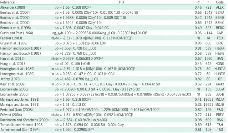
Table 1 − Published pedotransfer to estimate bulk density. Sample size (n) and R2 were taken from the original paper.
Reference PTF R2 n Code
Alexander (1980) ρb = 1.66 - 0.308 (OC)1/2 0.46 721 ALEX
Benites et al. (2007) ρb = 1.56 - 0.0005 (Clay*10) - 0.01 (OC*10) - 0.0075 SB 0.66 1542 BEN-A Benites et al. (2007) ρb = 1.5688 - 0.0005 (Clay*10) - 0.009 (OC*10) 0.42 1542 BEN-B
Benites et al. (2007) ρb = 1.5224 - 0.0005 (Clay*10) 0.63 1542 BEN-C
Bernoux et al. (1998) ρb = 1.398 - 0.0047 Clay - 0.042 OC 0.49 323 BERX
Curtis and Post (1964) Log10(ρb*100) = 2.09963-0.00064log10(LOI) - 0.22302 log10(LOI)2 0.96 ~144 C&P
Federer (1983) ln(ρb) = -2.31 - 1.079 ln[(OM/100)] - 0.113 ln[(OM/100)]2 NI NI FED
Grigal et al. (1989) ρb = 0.075 + 1.301exp (-0.06 LOI) 0.95 800 GRIG
Harrison and Bocock (1981) ρb =1.558 - 0.728 log10(LOI) 0.81 539 H&B-A
Harrison and Bocock (1981) ρb =1.729 - 0.769 log10(LOI) 0.58 538 H&B-B
Han et al. (2012) ln(ρb) = 0.5379 - 0.0653[(10 OM)]0.5 0.67 1560 HAN
Hong et al. (2013) ρb =1.02 - 0.156 ln(OM) 0.45 642 HONG
Huntington et al. (1989) ln ρb = -2.39 - 1.316 ln [(OM/100)] - 0.167 (ln [(OM/100)]2 0.75 60 HUNT-A
Huntington et al. (1989) ln ρb = 0.263 - 0.147 ln OC - 0.103 (ln OC)2 0.72 60 HUNT-B
Jeffrey (1970) ρb =1.482 - 0.6786 log10(LOI) 0.82 80 JEF
Kaur et al. (2002) ln ρb = 0.313 - 0.191 OC + 0.02102 Clay - 0.000476 (Clay)2 - 0.00432 Silt 0.62 224 KAUR
Leonavičiute (2000) ρb =1.70398 - 0.00313 Silt + 0.00261 Clay - 0.11245 OC NI 135 LEO-A Leonavičiute (2000) ρb = 1.07256 + 0.032732 ln(Silt) + 0.038753ln(Clay) + 0.078886 ln(Sand) - 0.054309 ln(OC) NI 858 LEO-B
Manrique and Jones (1991) ρb = 1.66 - 0.318 (OC)1/2 0.41 19651 M&J-A
Manrique and Jones (1991) ρb = 1.51 - 0.113 OC 0.36 19651 M&J-B
Perie and Ouim (2008) ρb = 1.977 + 4.105(OM/100) - 1.229ln[(OM/100)] - 0.103 ln[(OM/100)]2 0.82 125 P&O
Prévost (2004) ln(ρb) = -1.81 - 0.892*ln[(OM/100)] - 0.092 ln[(OM/100)]2 0.77 414 PREV
Ruehlmann and Körschens (2009) ρb = (2.684 - (140.943b)) exp(-bOC) 0.98 609 R&K
Tomasella and Hodnett (1998) ρb = 1.578 - 0.054 OC - 0.006 Silt - 0.004 Clay 0.59 613 T&H
Tamminen and Starr (1994) ρb = 1.565 - 0.2298(LOI)0.5 0.61 158 T&S
ρb = bulk density (g cm–3); OM = organic matter (%); OC = organic carbon (%); SB = sum of basic cations (cmol
c kg–1); LOI = loss-on-ignition (%); NI = not reported in
the original paper; b = coefficient for soil groups proposed by the authors (b = 0.006).
Figure 1 − Map with the location of points sampled.
The OC content was determined by using the elemental analyzer in Piracicaba, São Paulo, Brazil. Bulk density was obtained for each layer using the core method, by means of cylinders with volumetric rings 0.053 m high and 0.05 m in diameter. Detailed information can be found in Assad et al. (2013).
We eliminated samples that had a missing ρb val-ue or whose sum of particle size fractions (sand, silt, and clay) did not equal 100 %. The final data set consisted of 884 soil samples. The evaluation of the 25 PTFs was first performed by considering the whole data set (884 samples). In a second analysis, the data set was divided into two subgroups according to soil depth: the layer be-tween 0 and 10 cm (0-10 cm) and the layer bebe-tween 10 and 30 cm (10-30 cm).
Evaluation criteria
The most useful approach to an evaluation of predictive models should be based on a set of comple-mentary indices (Donatelli et al., 2004; Nanko et al., 2014). In the present study, the predictive capacity of the 25 PTFs was evaluated using the mean absolute error (MAE), RMSE, ME and R2. MAE is the value
overestimate or underestimate. R2 represents the
frac-tion of the total variance that is explained by the model. Higher R2 values are desirable.
Regression error characteristic curve - REC curve
The evaluation of the PTFs was complemented by the use of the REC curve. The regression error character-istic (REC) curve is a promising alternative for the evalu-ation of PTFs. The REC curve allows for comparisons of the performance of different models simultaneously using visual assessment, which facilitates interpretation by the user (Mittas and Angelis, 2010).
The REC curve represents the cumulative distri-bution function of the errors. On the x-axis the REC curve plots the error and on the y-axis the accuracy of a regression function (Mittas and Angelis, 2010). Accuracy is defined as the fraction of points that fit within an er-ror level, ranging from 0 to 1. Using this construction, we can evaluate the level of accuracy as the number of points for a given value of error.
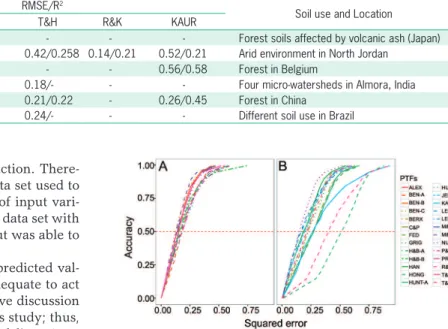
REC curves are built in a way that makes in-specting model performance a simple task of check-ing which model is closest to the (0, 1) point (up-per left corner) (Figure 2A). If the REC curve of one model is above the others, it is an indication that it is the best model for that metric, be it absolute error or squared error, or their relative forms (e.g., model c in Figure 2B). Thus, when comparing models a and b, if the REC curve from model a overlies the curve of model b, we can affirm that model a is superior to model b (Figure 2B). Model c in Figure 2B is superior to the others.
The REC curve also allows us to estimate the mod-el error by measuring the area over the curve (AOC). If the selected error measure is the squared error, the AOC corresponds to an underestimation of the mean squared error (MSE), and for the absolute error, the AOC corre-sponds to an underestimation of the MAE.
Finally, the REC curve allows for a comparison of the quality of a particular model with the simplest pos-sible estimation of an attribute from a population. In this study, the mean prediction corresponds to the simplest possible estimation of an attribute, and we used these values as a parameter to compare the performance of existing models. If the use of the mean values is better than a particular model, this model is not recommended
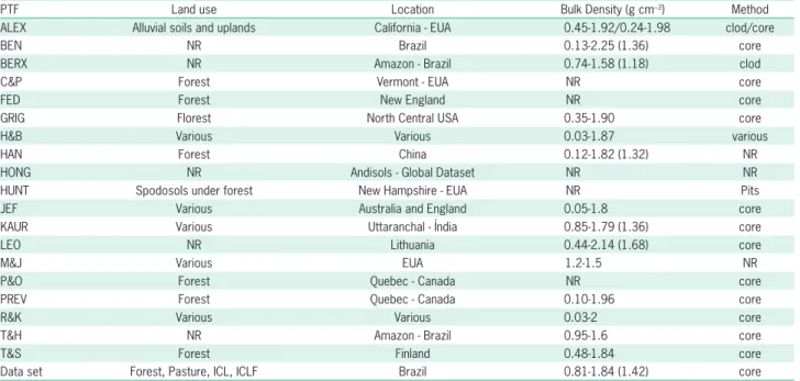
Table 2 − Land use, location, values of bulk density and method to determine bulk density for the data set used in the development of the tested
pedotransfer functions (PTFs). This information was taken from the original papers of the tested pedotransfer functions.
PTF Land use Location Bulk Density (g cm–3) Method
ALEX Alluvial soils and uplands California - EUA 0.45-1.92/0.24-1.98 clod/core
BEN NR Brazil 0.13-2.25 (1.36) core
BERX NR Amazon - Brazil 0.74-1.58 (1.18) clod
C&P Forest Vermont - EUA NR core
FED Forest New England NR core
GRIG Florest North Central USA 0.35-1.90 core
H&B Various Various 0.03-1.87 various
HAN Forest China 0.12-1.82 (1.32) NR
HONG NR Andisols - Global Dataset NR NR
HUNT Spodosols under forest New Hampshire - EUA NR Pits
JEF Various Australia and England 0.05-1.8 core
KAUR Various Uttaranchal - Índia 0.85-1.79 (1.36) core
LEO NR Lithuania 0.44-2.14 (1.68) core
M&J Various EUA 1.2-1.5 NR
P&O Forest Quebec - Canada NR core
PREV Forest Quebec - Canada 0.10-1.96 core
R&K Various Various 0.03-2 core
T&H NR Amazon - Brazil 0.95-1.6 core
T&S Forest Finland 0.48-1.84 core
Data set Forest, Pasture, ICL, ICLF Brazil 0.81-1.84 (1.42) core
NR = not reported in the original paper; ICL = integrated crop-livestock system; ICLF = integrated crop-livestock-forest system.
Figure 2 − A) Illustration of the Area Over Curve (AOC) of a model;
for that situation. The mean value will hereafter be re-ferred to as the null model.
When used in such manner, comparing models with REC curves is no different from using the MAE or RMSE. The benefits of the REC curve are related to oth-er easily visualized statistics, which can be the R2 or the
Kolmogorov-Smirnov Statistic to check if two samples are generated from the same distribution. Furthermore, the REC allows for quick visualization of the error me-dian (50 % horizontal line) or any level of confidence for different readers, e.g. one can look at the errors for 80 % confidence or 95 %.
REC curves were constructed following the steps proposed by Mittas and Angelis (2010): 1 – The model was set up, and the error in the predictions was evalu-ated; 2 – The error values were sorted in ascending or-der; 3 – For each error value that was not repeated, a point with the error value and the percentage of points with smaller errors were included in the graph. Step 1 was not necessary because we used available PTFs (Ta-ble 1). The RMSE was used as a measurement of error. Comparisons between curves were also made, by apply-ing the Wilcoxon signed rank test at the 0.05 level, with the Holm correction for multiple comparisons. This test assesses whether population mean ranks differ (paired difference test).
Results and Discussion
General evaluation
The descriptive statistics of the data set are shown in Table 3. The data set used has a wide range of ρb val-ues, with a minimum of 0.81 g cm–3, a maximum of 1.84 g
cm–3, and a mean value of 1.42 g cm–3 (Table 3). The PTFs
tested were developed from data sets with different uses, origins, ρb ranges and methods of determination (Table 2). The range of ρb values in the data set used for the com-parisons was within the range of values observed in the data sets used to generate the PTFs ALEX, BEN, GRIG, HAN, H&B, JEF, KAUR, LEO, PREV, R&K and T&S (Table 2 and Table 3). The PTFs BERX and HUNT used methods different from those used in this study; the PTFs ALEX and H&B used more than one method; and the PTFs HAN, HONG, and M&J did not inform the method used. The others used the core method.
The models performed differently when observed and estimated ρb values were compared (Figure 3 and Table 4). The ρb values were underestimated, except for the R&K, H&B-B and LEO (A and B) functions (Figure 3, Table 4). Underestimations in the prediction of ρb were also observed by De Vos et al. (2005), which they attrib-uted to the high proportion of topsoil data used in the calibration of the PTFs. These authors used forest soil data, in which the surface ρb tended to be lower than the subsurface values (Tamminen and Starr, 1994; De Vos et al., 2005), which can lead to underestimated ρb values. The data set used in this study are composed of soil data from the upper 30 cm of the soil profile, consid-ered as topsoil (De Vos et al., 2005; Martin et al., 2009). Additionally, 40 % of our data is from natural vegetation (ρb = 1.28 g cm–3) and integrated systems (crop-livestock ρb = 1.33 g cm–3; crop-livestock-forest ρb = 1.39 g cm–3),
which presented a lower topsoil ρb than pasture (ρb = 1.45 g cm–3). Data only from topsoil and under different
uses may explain the underestimates.
Lower ME values were observed for BEN-C and M&J-B indicating that these models were less biased (Table 4). The most biased models were HONG, R&K,
Table 3 − Descriptive statistics of the data set used to evaluate the 25 pedotransfer functions.
Statistics Silt Clay Sand OC OM ρb SB
--- % --- g cm–3 cmolc kg–1
All data set (n = 884)
Min-Max 1 - 67 0.1 - 76 2 - 95 0.1 - 8.3 0.2 - 13.2 0.81 - 1.84 0.3 - 30.5
Mean (Std dev) 17 28 55 1.4 2.5 1.42 4
Std dev 12 17 24 0.9 1.4 0.2 3.9
1st - 3rd quartile 9 - 22 15 - 40 38 - 73 0.7 - 1.8 1.5 - 3.1 1.26 - 1.56 1.6 - 5.1
Median 13 25 60 1.1 2.1 1.42 2.9
Topsoil (n = 442)
Min-Max 1 - 64 0.1 - 76 3 - 95 0.1 - 8.3 0.6 - 13.2 0.81 - 1.8 0.3 - 30.4
Mean (Std dev) 17 27 56 1.7 2.9 1.39 4.9
Std dev 12 17 24 1.1 1.6 0.2 4.1
1st - 3rd quartile 9 - 22 14 - 37 39 - 74 0.8 - 2.2 1.9 - 3.7 1.25 - 1.54 2.3 - 6.4
Median 13 24 62 1.4 2.7 1.4 3.7
Subsoil (n = 442)
Min-Max 1 - 67 0.2 - 76 2 - 95 0.1 - 4.6 0.2 - 8.6 0.88 - 1.84 0.3 - 30.5
Mean (Std dev) 17 30 54 1.1 1.9 1.41 3.2
Std dev 12 18 24 0.7 1.1 0.2 3.6
1st - 3rd quartile 9 - 22 16 - 42 35 - 72 0.6 - 1.5 1.2 - 2.4 1.26 - 1.57 1.2 - 4
Median 13 26 58 0.9 1.7 1.44 2.2
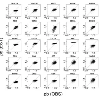
Figure 3 − Values observed (OBS) versus estimated (EST) of 25 PTFs (pedotransfer functions) evaluated in a data set of soils from different regions of Brazil with bulk density data for depths up to 30 cm. The dashed line corresponds to 1:1.
Table 4 − Mean absolute error (MAE), root mean squared error
(RMSE), mean error (ME), coefficient of determination (R2), and
area over the REC curve (AOC) with mean squared error (sqr) and with absolute error (abs) for published pedotransfer functions (PTFs) evaluated using bulk density data for all samples. The Wilcoxon Test was performed for differences between distributions of absolute errors.
All Data set
PTFs MAE RMSE ME R2 AOC_sqr AOC_abs Wilcoxon Test
HUNT-A 0.27 0.31 -0.24 0.05 0.10 0.27 hi HUNT-B 0.20 0.24 -0.17 0.34 0.06 0.20 bcd ALEX 0.15 0.19 -0.08 0.32 0.03 0.15 a M&J-A 0.16 0.19 -0.10 0.32 0.04 0.16 e M&J-B 0.14 0.17 -0.05 0.32 0.03 0.14 f T&H 0.16 0.19 -0.11 0.40 0.04 0.16 ae BERX 0.22 0.26 -0.19 0.31 0.07 0.22 g KAUR 0.31 0.38 -0.29 0.41 0.15 0.31 hi BEN-A 0.19 0.23 -0.15 0.35 0.05 0.19 bcd BEN-B 0.16 0.19 -0.10 0.35 0.04 0.16 e BEN-C 0.15 0.18 -0.02 0.19 0.03 0.15 f LEO-A 0.19 0.24 0.17 0.27 0.06 0.19 bcdkm LEO-B 0.20 0.25 0.17 0.32 0.06 0.20 bcdgkm R&K 0.42 0.47 0.42 0.31 0.22 0.42 n FED 0.27 0.31 -0.25 0.16 0.10 0.27 i T&S 0.22 0.26 -0.18 0.14 0.07 0.22 gm HAN 0.20 0.24 -0.14 0.14 0.06 0.20 b JEF 0.21 0.25 -0.14 0.12 0.06 0.21 k H&B-A 0.19 0.23 -0.08 0.12 0.05 0.19 c H&B-B 0.19 0.24 0.08 0.12 0.06 0.19 bcdek HONG 0.50 0.53 -0.50 0.12 0.28 0.50 l GRIG 0.23 0.23 -0.20 0.27 0.07 0.23 j C&P 0.26 0.30 -0.24 0.17 0.09 0.26 h PREV 0.19 0.23 -0.13 0.16 0.05 0.19 d P&O 0.19 0.24 -0.10 0.14 0.06 0.19 bd Null 0.17 0.20 0.00 NA 0.04 0.17 ae NA = not available; Null = null model; models followed by the same letter did not differ in the Willcoxon Signed Rank test at the 0.05 level with the Holm correction for multiple testing.
and KAUR. Out of the 12 models evaluated by De Vos et al. (2005), KAUR was the most biased and showed a high ME value. In the present study, this model had the third highest ME value (Table 4). The data used by De Vos et al. (2005) presented a ρb mean value (1.44 g cm–3) very
similar to the data used here (1.42 g cm–3). However, the
range of ρb (0.22 to 1.96 g cm–3) was wider than what we
recorded (0.81 to 1.84 g cm–3). On the other hand, the
most biased models tested by Nanko et al. (2014) were H&B and ALEX, which were among the models with lower values. They used data from volcanic soils, with a range of ρb between 0.13 and 1.78 g m–3 and a very low
mean of 0.6 g cm–3.
The best indices (MAE, RMSE, and ME) were observed in the M&J-B, ALEX, BEN-B, BEN-C, M&J-A and T&H models. Out of the models with lower errors (MAE, RMSE, and ME), the T&H model had the high-est R2 value and, therefore, represented a more realistic
model. When considering the models developed from the data from Brazilian soils (BEN-A, BEN-B, BEN-C, BERX, and T&H), we observed that three of them are among the best models: BEN-B, BEN-C and T&H.
The worst indices were observed in the HONG, R&K, and KAUR models. Furthermore, HONG, R&K, BEN-C, LEO-B, and C&P models provided similar esti-mates of ρb (Figure 3) for a data set with a broad range of values (0.86 g cm–3 to 1.8 g cm–3) (Table 3). This
find-ing reveals that these models do not provide reliable pre-dictions of ρb. The performance of the PTFs using data sets that differ from those used in their development is uncertain and may not be satisfactory, especially when the data sets are sourced from different geographic areas (Wösten et al., 2001) (Table 5).
In addition to the difficulty associated with extrap-olating these models due to the specificity of the data sets used in their development (Table 3), the method used to generate the PTFs also appears to affect the re-sults (Martin et al., 2009; Jalabert et al., 2010; Suuster et al., 2011). These methods are quite varied, ranging from simple regressions to more powerful methods such as neural networks, regression trees (Martin et al., 2009; Jalabert et al., 2010; Ghehi et al., 2012), and the nearest-neighbor method (Nemes et al., 2010). In the case of the PTFs assessed in our study, the methods used were mostly simple or multiple regressions using the least squares method.
only OC or OM and one granulometry fraction. There-fore, when considering the origin of the data set used to develop the model, the number, and type of input vari-ables, the model generated from a Brazilian data set with OC and two granulometry fractions as input was able to predict ρb more effectively.
When comparing the observed and predicted val-ues, certain patterns in results appear inadequate to act as a good predictor (Figure 3). An exhaustive discussion of these patterns is beyond the scope of this study; thus, two patterns were observed: the horizontal lines (e.g., BEN-C) and the 'flat top' (e.g., HUNT-A). The horizon-tal line found in BEN-C is easily explained by the small magnitude of the angular coefficients (10–3-10–5)
com-pared with the linear coefficient (1.5688). Although the data set used in this study contains ρb values between 0.81 and 1.84 g cm–3, the BEN-C model predicted
val-ues between 1.14 and 1.51 g cm–3. This range is even
narrower for the LEO-B model, which predicted values between 1.33 and 1.71 g cm–3. The previous analysis
de-veloped for BEN-C and LEO-B can be extended to the R&K and C&P models.
The 'flat top' pattern was observed in the HUNT-A, HUNT-B, and KAUR models and, to a lesser extent, in LEO-A and FED. An evaluation of the parameters of the HUNT-A equation and the values of the data set al-lowed us to conclude that the predicted values would lie between 1.04 and 1.36 g cm–3. The maximum value is
lower than the average ρb value for the data set (1.42 g cm–3), resulting in a flat aspect on the graph.
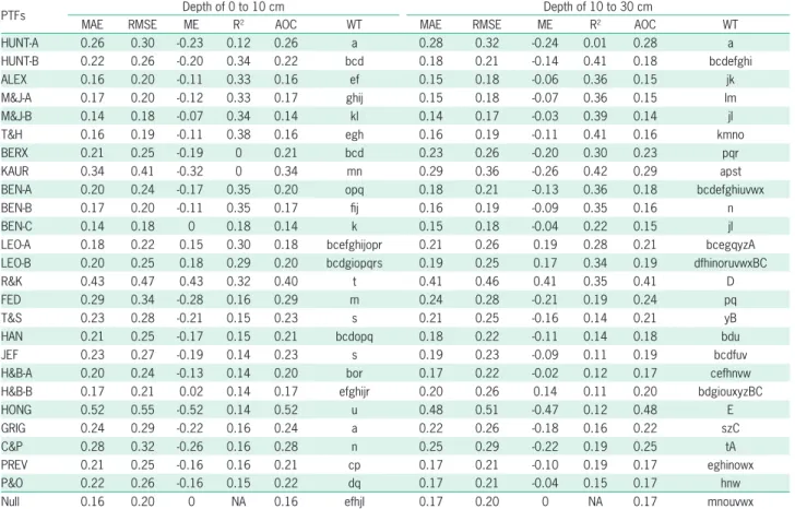
When the data set was separated according to depth (0-10 cm and 10-30 cm), the values of the indi-ces showed only slight variations (Table 6). The M&J-B, BEN-B, BEN-C, ALEX, M&J-A, and T&H continued to perform well, and the HONG, R&K, and KAUR models had the worst performance. The lowest RMSE values were observed for the BEN-C and M&J-B and the high-est for the HONG model for both soil depths.
REC curve
In the evaluation using the REC curve, the models were separated into different graphs for easier visualiza-tion (Figure 4A and B). The 12 best models are presented in Figure 4A and the remainder in Figure 4B. Table 4 also presents the values of AOC calculated from squared error (AOC_square) and absolute error (AOC_abs), and
the results of the comparisons of the REC curves by the Wilcoxon test at the 0.05 level with the Holm correction for multiple testing.
Among the 12 best models, the Wilcoxon test showed that ALEX, BEN-B, H&B-B, M&J-A and T&H models presented a distribution similar to the null model. Otherwise, HUNT-B, H&B-A, BEN-A, PREV, and P&O models presented a different distribution from the null model, with an inferior performance for the majority of the error range (Figure 4A and Table 4). BEN-C and M&J-B also presented a different dis-tribution from the null model, with a superior per-formance for a particular range of errors. The better performance of the M&J-B model is likely due to the variability of the data used in its generation (12,000 soil profiles) (Manrique and Jones, 1991). The result for BEN-C is probably related to similarity between data sets (Benites et al., 2007).
The 13 worst models presented a distribution dis-similar from the null model, with an inferior performance for the whole error range, showing that these models have low predictive ability (Figure 4B and Table 4). The HONG, R&K, and KAUR models had the worst results, with much poorer performance than the null model (Fig-ure 4B and Table 4). De Vos et al. (2005) observed poor performance for both the KAUR and HUNT models using forest soil data from Belgium. These models were
devel-Table 5 − RMSE (root mean squared error) (First value) and R2 (Second value) for the PTFs (pedotransfer functions) Alexander et al. (1980) (ALEX),
Manrique and Jones (1991) (M&J) and Tomasella and Hodnett (1998) (T&H) and Kaur et al. (2002) (KAUR), when applied to different data sets.
References RMSE/R2 Soil use and Location
ALEX M&J T&H R&K KAUR
Nanko et al. (2014) 0.32/0.64 0.30/0.64 - - - Forest soils affected by volcanic ash (Japan) Al-Qinna and Jaber (2013) 0.33/0.22 0.34/0.23 0.42/0.258 0.14/0.21 0.52/0.21 Arid environment in North Jordan De Vos et al. (2005) 0.30/0.58 0.32/0.58 - - 0.56/0.58 Forest in Belgium
Kaur et al. (2002) 0.19/- 0.20/- 0.18/- - - Four micro-watersheds in Almora, India Han et al. (2012) 0.14/0.59 0.35/0.46 0.21/0.22 - 0.26/0.45 Forest in China
Benites et al. (2007) - 0.27/- 0.24/- - - Different soil use in Brazil
Figure 4 − REC (regression error characteristic) curve for the 25
oped for very specific conditions, making them difficult to extrapolate (Table 2). Furthermore, the HUNT model used different methods to determine the ρb.
Nemes et al. (2010) emphasize that the model se-lected should be one developed from similar areas as regards soil genesis. However, even the PTFs developed for Brazilian soils, such as those generated by Benites et al. (2007), showed a performance slightly superior to the null model and for specific conditions.
The Wilcoxon test for REC curves according to depth showed similar results when considering all the data set (Table 6). For depths up to 10 cm (Figure 5A and B), ALEX, BEN-B, H&B-B, M&J-A, and T&H, together with M&J-B and LEO-A models, continued to present a distribution similar to the null model (Table 6). The BEN-C was the only model with a distribution different from the null model, but, again the gain in their applica-tion was very small and only for specific error ranges. The other five models, out of the 12 best ones HUNT-B, BEN-A, H&B-A, PREV, and P&O, presented a distribu-tion different from the null model, with inferior perfor-mance for the majority of the error range (Figure 5A).
Table 6 − Mean absolute error (MAE), root mean squared error (RMSE), mean error (ME), coefficient of determination (R2) and area over de REC
curve (AOC) with absolute error for published pedotransfer functions (PTFs) evaluated using bulk density data for two classes of depth (0 to 10 cm and 10 to 30 cm). The Wilcoxon Test (WT) was performed for differences between distributions of absolute errors.
PTFs Depth of 0 to 10 cm Depth of 10 to 30 cm
MAE RMSE ME R2 AOC WT MAE RMSE ME R2 AOC WT
HUNT-A 0.26 0.30 -0.23 0.12 0.26 a 0.28 0.32 -0.24 0.01 0.28 a
HUNT-B 0.22 0.26 -0.20 0.34 0.22 bcd 0.18 0.21 -0.14 0.41 0.18 bcdefghi
ALEX 0.16 0.20 -0.11 0.33 0.16 ef 0.15 0.18 -0.06 0.36 0.15 jk
M&J-A 0.17 0.20 -0.12 0.33 0.17 ghij 0.15 0.18 -0.07 0.36 0.15 lm
M&J-B 0.14 0.18 -0.07 0.34 0.14 kl 0.14 0.17 -0.03 0.39 0.14 jl
T&H 0.16 0.19 -0.11 0.38 0.16 egh 0.16 0.19 -0.11 0.41 0.16 kmno
BERX 0.21 0.25 -0.19 0 0.21 bcd 0.23 0.26 -0.20 0.30 0.23 pqr
KAUR 0.34 0.41 -0.32 0 0.34 mn 0.29 0.36 -0.26 0.42 0.29 apst
BEN-A 0.20 0.24 -0.17 0.35 0.20 opq 0.18 0.21 -0.13 0.36 0.18 bcdefghiuvwx
BEN-B 0.17 0.20 -0.11 0.35 0.17 fij 0.16 0.19 -0.09 0.35 0.16 n
BEN-C 0.14 0.18 0 0.18 0.14 k 0.15 0.18 -0.04 0.22 0.15 jl
LEO-A 0.18 0.22 0.15 0.30 0.18 bcefghijopr 0.21 0.26 0.19 0.28 0.21 bcegqyzA LEO-B 0.20 0.25 0.18 0.29 0.20 bcdgiopqrs 0.19 0.25 0.17 0.34 0.19 dfhinoruvwxBC
R&K 0.43 0.47 0.43 0.32 0.40 t 0.41 0.46 0.41 0.35 0.41 D
FED 0.29 0.34 -0.28 0.16 0.29 m 0.24 0.28 -0.21 0.19 0.24 pq
T&S 0.23 0.28 -0.21 0.15 0.23 s 0.21 0.25 -0.16 0.14 0.21 yB
HAN 0.21 0.25 -0.17 0.15 0.21 bcdopq 0.18 0.22 -0.11 0.14 0.18 bdu
JEF 0.23 0.27 -0.19 0.14 0.23 s 0.19 0.23 -0.09 0.11 0.19 bcdfuv
H&B-A 0.20 0.24 -0.13 0.14 0.20 bor 0.17 0.22 -0.02 0.12 0.17 cefhnvw H&B-B 0.17 0.21 0.02 0.14 0.17 efghijr 0.20 0.26 0.14 0.11 0.20 bdgiouxyzBC
HONG 0.52 0.55 -0.52 0.14 0.52 u 0.48 0.51 -0.47 0.12 0.48 E
GRIG 0.24 0.29 -0.22 0.16 0.24 a 0.22 0.26 -0.18 0.16 0.22 szC
C&P 0.28 0.32 -0.26 0.16 0.28 n 0.25 0.29 -0.22 0.19 0.25 tA
PREV 0.21 0.25 -0.16 0.16 0.21 cp 0.17 0.21 -0.10 0.19 0.17 eghinowx
P&O 0.22 0.26 -0.16 0.15 0.22 dq 0.17 0.21 -0.04 0.15 0.17 hnw
Null 0.16 0.20 0 NA 0.16 efhjl 0.17 0.20 0 NA 0.17 mnouvwx
NA = not available; Null = null model; models followed by the same letter did not differ in the Willcoxon Signed Rank test at the 0.05 level with the Holm correction for multiple testing.
Figure 5 − REC (regression error characteristic) curve for the 25
For depths of 10 to 30 cm (Figure 5C and D), the Wilcoxon test showed that 10 of the 12 best models did not differ from the null model (Table 6). A slight improvement occurred with the application of ALEX, M&J-B, BEN-B, and BEN-C models, but also for a par-ticular error range and, therefore, cannot be interpreted as better performance of these models compared to the null model (Figure 5C). Previous studies have shown the influence of soil depth on the prediction of ρb. De Vos et al. (2005) found a 24 % improvement in the performance of PTFs in RMSE for ρb prediction at greater depths. Heuscher et al. (2005) noted that depth was responsible for approximately 1 % of the variation in ρb, and the greatest variation observed was 7 %. Benites et al. (2007) did not observe an improvement in the accuracy of the PTFs after separating the soils by depth (0 to 30 cm and 30 to 100 cm). Tranter et al. (2007) found better results when using the depth expressed on a logarithmic scale. Nemes et al. (2010) observed a decrease in the bias after separating the soil by depth.
In general, only BEN-C presented a slight im-provement in ρb estimates for all situations (all data set, depths up to 10 cm and depths of 10 to 30 cm), when compared to the null model. The number of models with better results for topsoil was more restricted than for the subsurface. Having a worse performance for the topsoil as compared with the subsurface soil raises con-cerns as regards the estimation of soil C stock in which 0 to 30 cm are commonly considered as a reference layer (IPCC, 1997). Given the higher concentration of OC in the surface compared to the lower layer (Table 3), the error will be greater where it matters most.
The method used to determine the predictors of a PTF or the estimated variable (ρb) also seems to af-fect their performance. Both ρb and OC (or OM) can be measured by different methodologies (Sleutel et al., 2007; Blake and Hartge, 1986). The LOI and wet-oxidation methods are the two most commonly used methods for quantifying OM. However, the LOI meth-od has no standard protocol and involves potentially confounding factors (Hoogsteen et al., 2015) even if the granulometric data could present variations since na-tional and internana-tional classification systems often use quite different particle size ranges. In fact, Wösten et al. (2001) pointed out that there is no single source of variability, either PTF-related or soil-related, that can explain the uncertainty in every calculated functional aspect of soil behavior. The authors suggest using large and reliable data sets as well as PTFs developed from soils with similar attribute ranges to those used for the predictions. Here, we could see that similar ranges of soil attributes are not a guarantee of good predictions. The REC curve allows us to show that the 12 PTFs with the best indices presented, in general, a perfor-mance similar to the null model. BEN-C and M&J-B models presented the best results. The improvements observed were insignificant and were found only in specific error ranges.
Conclusions
The 25 models tested performed differently when observed and estimated bulk density values are com-pared, and the BEN-C and M&J-B models presented the best results.
The separation of data into two layers according to depth (0-10 cm and 10-30 cm) demonstrated a worse per-formance for the 0-10 cm layer, which raises concerns about the estimation of soil C in the upper layers that contain most of the organic matter.
The use of the REC curve as a form of analysis allowed for a simple and visual evaluation of the perfor-mance of the models.
The pedotransfer functions tested in this study showed a performance close to that of the null model (mean value) when estimating bulk density for soils from different regions of Brazil, indicating little or no additional benefit from the use of the null model.
Acknowledgements
We thank FAPESP (São Paulo Research Foundation) for financial support (Registry numbers: 2015/06804-0) and CNPq (Brazilian National Council for Scientific and Technological Development) for productivity grants in research to Eduardo Delgado Assad.
References
Alexander, E.B. 1980. Bulk densities of California soils in relation to other soil properties. Soil Science Society of America Journal 44: 689-692.
Alletto, L.; Coquet, Y. 2009. Temporal and spatial variability of soil bulk density and near-saturated hydraulic conductivity under two contrasted tillage management systems. Geoderma 152: 85-94. Al-Qinna, M.I.; Jaber, S.M. 2013. Predicting soil bulk
density using advanced pedotransfer functions in an arid environment. Transactions of the ASABE 56: 963-976. Assad, E.D.; Pinto, H.S.; Martins, S.C.; Groppo, J.D.; Salgado,
P.R.; Evangelista, B.; Vasconcelos, E.; Sano, E.E.; Pavão, E.; Luna, R.; Camargo, P.B.; Martinelli, L.A. 2013. Changes in soil carbon stocks in Brazil due to land use: paired site comparisons and a regional pasture survey. Biogeosciences 10: 1-22. Benites, V.M.; Machado, P.L.O.A.; Fidalgo, E.C.C.; Coelho, M.R.; Madari,
B.E. 2007. Pedotransfer functions for estimating soil bulk density from existing soil survey reports in Brazil. Geoderma 139: 90-97.
Bernoux, M.; Arrouays, D.; Cerri, C.; Volkoff, B.; Jovilet, C. 1998. Bulk densities of Brazilian Amazon soils related to other soil properties. Soil Science Society of America Journal 62: 743-749. Bouma, J. 1989. Using soil survey data for quantitative land
evaluation. Advances in Soil Science 9: 177-213.
Black, G.R.; Hartge, K.H. Bulk Density. In: Klute, A. (Ed.). Methods of soil analysis: Physical and Mineralogical Methods. Part 1. Madison: American Society of Agronomy, 1986. p. 363-375. Curtis, R.O.; Post, B.W. 1964. Estimating bulk density from
De Vos, B.; Meirvenne, M.V.; Quataert, P.; Deckers, J.; Muys, B. 2005. Predictive quality of pedotransfer functions for estimating bulk density of forest soils. Soil Science Society of America Journal 69: 500-510.
Dexter, A.R. 2004. Soil physical quality. Part I. Theory, effects of soil texture, density, and organic matter, and effects on root growth. Geoderma 120: 201-214.
Donatelli, M.; Acutis, M.; Nemes, A.; Wosten, H. 2004. Methods to evaluate pedotransfer function: integrated indices for pedotransfer function. p. 357-414. In: Pachepsky, Y.A.; Rawls, W.J., eds. Development of pedotransfer function in soil hydrology. Elsevier Science, Amsterdam, The Netherlands. Empresa Brasileira de Pesquisa Agropecuária [Embrapa]. 1997.
Manual of Methods for Soil Analysis = Manual de Métodos de Análise de Solo. Centro Nacional de Pesquisa de Solos, Rio de Janeiro, RJ, Brazil (in Portuguese).
Federer, C.A. 1983. Nitrogen mineralization and nitrification: depth variation in four New England forest soils. Soil Science Society of America Journal 47: 1008-1014.
Ghehi, N.G.; Nemes, A.; Verdoodt, A.; Van Ranst, E.; Cornelis, W.M.; Boeckx, P. 2012. Nonparametric techniques for predicting soil bulk density of tropical rainforest topsoils in Rwanda. Soil Science Society of America Journal 76: 1172.
Grigal, D.F.; Brovold, S.L.; Nord, W.S.; Ohmann, L.F. 1989. Bulk density of surface soils and peat in the north central United States. Canadian Journal of Soil Science 90: 895-900.
Han, G.Z.; Zhang, G.L.; Gong, Z.T.; Wang, G.F. 2012. Pedotransfer functions for estimating soil bulk density in China. Soil Science 177: 158-164.
Harrison, A.F.; Bocock, K.L. 1981. Estimation of soil bulk-density from loss-on-ignition values. Journal of Applied Ecology 18: 919-927.
Heuscher, S.A.; Brandt, C.C.; Jardine, P.M. 2005. Using soil physical and chemical properties to estimate bulk density. Soil Science Society of America Journal 69: 1-7.
Hong, S.Y.; Minasny, B.; Han, K.H.; Kim, Y.; Lee, K. 2013. Predicting and mapping soil available water capacity in Korea. Peer Journal 1: e71.
Hoogsteen, M.J.J.; Lantinga, E.A.; Bakker, E.J.; Groot, J.C.J.; Tittonell, P.A. 2015. Estimating soil organic carbon through loss on ignition: effects of ignition conditions and structural water loss. European Journal of Soil Science 66: 320-328.
Huntington, T.G.; Johnson, C.E.; Johnson, A.H.; Siccama, T.G.; Ryan, D.F. 1989. Carbon, organic matter, and bulk density relationships in a forested spodosol. Soil Science 148: 380-386. Intergovernmental Panel on Climate Change [IPCC]. 1997. Revised
1996 IPCC Guidelines for National Greenhouse Gas Inventories. IPCC, Paris, France.
Jalabert, S.S.M.; Martin, M.P.; Renaud, J.P.; Boulonne, L.; Jolivet, C.; Montanarella, L.; Arrouays, D. 2010. Estimating forest soil bulk density using boosted regression modelling. Soil Use Management 26: 516-528.
Jeffrey, D.W. 1970. A note on the use of ignition loss as a means for the approximate estimation of soil bulk density. Journal of Ecology 58: 297-299.
Kaur, R.; Kumar, S.; Gurung, H. 2002. A pedo-transfer function (PTF) for estimating soil bulk density from basic soil data and its comparison with existing PTFs. Australian Journal of Soil Research 40: 847-857.
Leonavičiute, N. 2000. Predicting soil bulk and particle densities
by pedotransfer functions from existing soil data in Lithuania. Geografijos metraštis 33: 7-330.
Manrique, L.A.; Jones, C.A. 1991. Bulk density of soils in relation to soil physical and chemical properties. Soil Science Society of America Journal 55: 476-481.
Martin, M.P.; Lo Seen, D.; Boulonne, L.; Jolivet, C.; Nair, K.M.; Bourgeon, G.; Arrouays, D. 2009. Optimizing pedotransfer functions for estimating soil bulk density using boosted regression trees. Soil Science Society of America Journal 73: 485-493.
Mittas, N.; Angelis, L. 2010. Visual comparison of software cost estimation models by regression error characteristic analysis. Journal of Systems and Software 83: 621-637.
Mouazen, A.M.; Ramon, H.; Baerdemaeker, J.D. 2003. Modelling compaction from on-line measurement of soil properties and sensor draught. Precision Agriculture 4: 203-212.
Nanko, K.; Ugawa, S.; Hashimoto, S.; Imaya, A.; Kobayashi, M.; Sakai, H.; Ishizuka, S.; Miura, S.; Tanaka, N.; Takahashi, M.; Kaneko, S. 2014. A pedotransfer function for estimating bulk density of forest soil in Japan affected by volcanic ash. Geoderma 213: 36-45.
Nemes, A.; Quebedeaux, B.; Timlin, D.J. 2010. Ensemble approach to provide uncertainty estimates of soil bulk density. Soil Science Society of America Journal 74: 1938-1945. Périé, C.; Ouimet, R. 2008. Organic carbon, organic matter and
bulk density relationships in boreal forest soils. Canadian Journal of Soil Science 88: 315-325.
Prévost, M. 2004. Predicting soil properties from organic matter content following mechanical site preparation of forest soils. Soil Science Society of America Journal 68: 943-949.
Ruehlmann, J.; Körschens, M. 2009. Calculating the effect of soil organic matter concentration on soil bulk density. Soil Science Society of America Journal 73: 876-885.
Sleutel, S.; Neve, S.; Singier, B.; Hofman, G. 2007. Quantification of organic carbon in soils: a comparison of methodologies and assessment of the carbon content of organic matter. Communication in Soil Science and Plant Analysis 38: 2647-2657.
Suuster, E.; Ritz, C.; Roostalu, H.; Reintam, E.; Kõlli, R.; Astover, A. 2011. Soil bulk density pedotransfer functions of the humus horizon in arable soils. Geoderma 163: 74-82.
Tamminen, P.; Starr, M. 1994. Bulk density of forested mineral soils. Silva Fennica 28: 53-60.
Tomasella, J.; Hodnett, M.G. 1998. Estimating soil water retention characteristics from limited data in Brazilian Amazonia. Soil Science 163: 190-202.
Tranter, G.; Minasny, B.; McBratney, A.B.; Murphy, B.; Mckenzie, N.J.; Grundy, M.; Brough, D. 2007. Building and testing conceptual and empirical models for predicting soil bulk density. Soil Use Management 23: 437-443.