On the Nondegeneracy Theorem for a Particle in a Box
Salvatore De Vincenzo Escuela de F´ısica, Facultad de Ciencias,
Universidad Central de Venezuela, A.P. 47145, Caracas 1041-A, Venezuela
E-mail: [email protected] (Received on 14 July, 2008)
We present some essential results for the Hamiltonian of a particle in a box. We discuss the invariance of this operator under time-reversal ˆT, the possibility of choosing real eigenfunctions for it and the degeneracy of its energy eigenvalues. Once these results have been presented, we introduce the usual nondegeneracy theorem and discuss some issues surrounding it. We find that the nondegeneracy theorem is true if the boundary conditions are ˆT-invariant but “confining” (i.e., the particle is in a real impenetrable box). If the boundary conditions are not ˆT-invariant (belonging to a family of so-called “not confining” boundary conditions), the respective eigenfunctions are strictly complex and there is no degeneracy. Consistently, we verify the validity of the theorem also in this case. Finally, if the boundary conditions are also ˆT-invariant, but “not confining”, then we can have degeneracy in the energy levels only if the respective eigenfunctions can be specifically written as complex. We find that the nondegeneracy theorem fails in these cases. If the respective eigenfunctions can be written as only real, then we do not have degeneracy and the nondegeneracy theorem is true.
Keywords: Quantum Mechanics; Particle in a box; Nondegeneracy theorem; Time-reversal invariance
1. INTRODUCTION
Some time ago, Loudon [1], in studying the one-dimensional model of a hydrogen atom (V(x) =−k/|x|), found that all of the discrete energy levels turn out to be dou-bly degenerate; that is, two different eigenfunctions have the same energy. Likewise, Loudon himself pointed out that the usual proof that forbids the degeneracy for a one-dimensional system, which seemed to be independent of the shape of the potential did not apply to the case he was treating. A later, more carefully study, gave several arguments that seemed to confirm that these discrete energy levels could not be degen-erate [2]. More recently, Cohen and Kuharetz studied another example of a one-dimensional system: An infinite square well with a singular potential (actually proportional to the Dirac delta) with adjustable strength at the center of the well [3]. The solution had doubly degenerate energy eigenvalues. It is worth mentioning that the trouble with the degeneracy in this system had already been mentioned by Oseguera [4]. These aspects have also been considered in the context of super-symmetric quantum mechanics [5]. All of these results ap-parently prove that the so-called nondegeneracy theorem is not necessarily valid for potentials that have a singular point. In spite of this fact, the proof of this theorem in some books makes no mention of this specific point [6]. We recently found another reference in which the appearance of degeneracy in the presence of certain singular potentials is explored in one-dimensional quantum systems, although the authors of this reference also showed cases of nondegeneracy in the presence of singular potentials [7]. We have also seen a study that found that bound states, degenerate in energy, may exist even if the potential is unbounded from below at infinity [8].
However, there exists another one-dimensional system with real and complex eigenfunctions that is much more simple than any mentioned above and, depending on the boundary conditions, it can present double degeneracy in its energy lev-els. This is the well known problem of a particle in the closed
interval 0≤x≤πwith a potential of zero inside the box. (In-cidentally, as the motion of the particle remains, in this case, limited or restricted to[0,π], we consider the Hilbert space L2([0,π]), where[0,π]⊂ℜ. The quantum mechanical treat-ment of the infinite square well potential with Hilbert space L2(ℜ), with the functions in the respective domain of the Hamiltonian vanishing ifx<0 andx>π, is not equivalent to the problem inL2([0,π]). In such a way that, the usual non-degeneracy theorem does not always work for a particle in a box and, for this reason, it is important to study all of the is-sues surrounding this result carefully. This is one of the goals of the present paper.
The ordinary differential equation (ODE) for the eigenval-ues (and eigenfunctions) in our problem is ˆLu(x) +λu(x) =0, where ˆL=d2/dx2is a self-adjoint (hermitian) operator with u(x)satisfying some of the following boundary conditions [9-13]. The Hamiltonian of the system is ˆH=−Lˆ with energy E=λ; moreover~2=2m=1:
µ
u(π)−iηu′(π)
u(0) +iηu′(0) 
=U µ
u(π) +iηu′(π)
u(0)−iηu′(0) 
. (1)
The primes denote differentiation with respect tox; the pa-rameterηis inserted for dimensional reasons and the matrix U, belonging toU(2), can be written, in this instance, as [12]:
U=exp(iφ) µ
m0−im3 −m2−im1
m2−im1 m0+im3
, (2)
whereφ∈[0,π], and the quantitiesmk∈ℜ (k=0,1,2,3.)
j(x) =1 i
µ ¯ u(x)d
dxu(x)−u(x) d dxu(x)¯
The bars denote complex conjugation. This satisfies j(0) = j(π), and this condition is equivalent to the self-adjointness of the Hamiltonian. For some of these boundary conditions we have j(0) = j(π) =0 by necessity, which is the impenetra-bility condition at the walls of the box (see, for example, [9] and [10]). In fact, we found an expression for the probability current density at the walls of the box:
j(0) =j(π) =−1 η
· 1 m0+cos(φ)
¸
Re[(m2+im1)u(0)u(π)]¯ . (3) Notice that, by setting m1=m2=0, we obtain j(0) =
j(π) =0. (See, for example, [9] and [14] for other comments about this fact, although we have a different parameterization for the matrixU in equation (2)). The respective subfamily of (“general” unmixed) confining boundary conditions, which correspond to a particle in a real impenetrable box, can be written (from (1) and (2)) as:
u(π) +ηcot((φ−θ)/2)u′(π) =0,
u(0)−ηcot((φ+θ)/2)u′(0) =0, (4) whereθ=tan−1(m3/m0). Note that this subfamily of bound-ary conditions is similar to that studied and termed “sepa-rated” by Albeverioet al[15,16] for a free particle on a line with a hole (i.e., a point interaction).
From (3) it is clear that if the eigenfunctions are real func-tions withm2=0 andm16=0, then we also havej(0) =j(π) = 0. Consistently, if the Hamiltonian operator ˆHis invariant un-der time-reversal ˆT, we have(Tˆ−1Hˆ T u)(x) = (ˆ Hu)(x)ˆ , so that the operator ˆT commutes with ˆH, and the time-reversal transformed function must satisfy(T u)(x)ˆ ∈D(H)ˆ . If we con-sider a stationary state of definite energy (in this case, ˆTis also called the complex conjugation operator), this invariance im-plies thatu(x)and(u)(x)¯ ≡(T u)(x)ˆ are two eigenfunctions of
ˆ
Hwith the same eigenvalue, and that they both comply with the same boundary condition. Thus, the matrixUmust satisfy U+=U¯, which impliesm2=0 [12]. Therefore, the number of the parameters inUis reduced to three, and the eigenfunctions for these ˆT-invariant Hamiltonians can be real functions. This result has also been found for the problem of a particle on a line with a hole; see [17] and references therein. Note that, all of the boundary conditions included in the so-called confining family (4) are automatically ˆT-invariant as well. However, we will prove specifically that they do not lead to degeneracy in the energies. Therefore in this case, we necessarily obtain real eigenfunctions with their respective zero probability currents.
Thus, as u and ¯u are (different) complex eigenfunctions of ˆH with the same eigenvalue (or Re(u) = (u+u)¯ /2 and Im(u) = (u+u)¯ /2ibelonging toℜ), there is a double degener-acy in the energy levels; therefore, the usual proof that forbids the degeneracy for a one-dimensional system [6] must be re-examined in light of the problem of a particle inside a box. A necessary condition for the existence of degeneracy in the en-ergies in this problem is that the corresponding Hamiltonian be invariant under time-reversal. Hence, there must also exist
ˆ
T-invariant boundary conditions which do not lead to degen-eracy in the energies; i.e., asuand ¯udiffer only by a constant factor and therefore represent the same state, Re(u)and Im(u) must also represent the same state. In other words, there is only one unique eigensolution for each eigenvalue of the en-ergy, so we can always choose this eigensolution to be real. If the (complex or real) eigenfunctions of the Hamiltonian ˆHare doubly degenerate, then the respective boundary condition is
ˆ
T-symmetric. If the boundary condition is not ˆT-symmetric, then the eigenfunctions must be necessarily complex and, in addition, they cannot be degenerate.
When the probability current density is not null at the walls of the box (see relation (3)), we can say that (physically) the walls are transparent to the current. In some of these cases, the underlying classical particle arrives at one wall and then ap-pears at the other (see references in [18] for comments about this point). We can therefore write a second family of bound-ary conditions; this one may be called, say, “not confining”, but only if the respective eigenfunctions are (written as) com-plex functions and are therefore degenerate, if they are ˆT -invariant; or not degenerate, if they are not ˆT-invariant. Note that the probability current is not zero only if the respective functions are complex functions because real functions always lead to zero probability current inside the box. Thus, if the particle is not really confined to the box, the wave function must be complex (we read a very slight comment about this point in [19], page 2, after the equation (7)). Finally, this “not confining” family, together with the family (4) (as well as the general boundary condition (1)) compose the whole family of boundary conditions for the self-adjoint Hamiltonian for a particle in a box (see the article by V. Alonsoet al, in [14]):
µ u(π) ηu′(π)
¶ =M
µ u(0) ηu′(0)
, (5)
where the matrixMis:
M= i
−m2+im1
µ
m3+sin(φ) −m0−cos(φ) −m0+cos(φ) −m3−sin(φ)
. (6)
M=exp¡
i(tan−1(m1/m2) + (π/2))¢
1 p
(m1)2+ (m2)2
µ
m3+sin(φ) −m0−cos(φ) −m0+cos(φ) −m3+sin(φ)
,
which confirms, due to the relation(m0)2+ (m1)2+ (m2)2+
(m3)2=1, thatMdoes belong to the groupU(1)×SL(2,ℜ). Moreover, the elements in the matrixM can have only finite values (that is,m1andm2cannot be simultaneously null). By the way, the subfamily of boundary conditions (5) is similar to the “connected” subfamily of boundary conditions studied by Albeverioet al[15,16] for a free particle on a line with a point interaction. Lastly, note that all of the coefficients in the matrixMare real for ˆT-invariant boundary conditions (since onlym2=0).
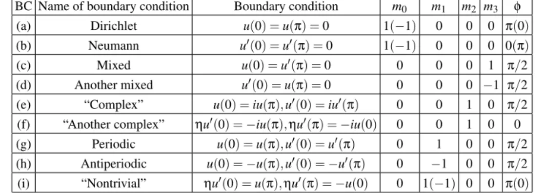
For examples of boundary conditions included in (1), see Table 1. Within the confining subfamily (4), we have, for ex-ample: (a) The usual Dirichlet boundary condition, u(0) = u(π) =0; (b) the Neumann boundary condition, u′(0) = u′(π) =0; and the so-called mixed boundary conditions, (c) u(0) =u′(π) =0 and (d)u′(0) =u(π) =0. These four ˆT -invariant boundary conditions do not lead to degeneracy in the energies (see Table 2) and satisfym1=m2=0. There-fore, there is a valid place for the nondegeneracy theorem.
As examples of boundary conditions which are not ˆT -symmetric, we have: (e) one complex condition: u(0) = iu(π),u′(0) =iu′(π); (f) and another odd condition,ηu′(0) = −iu(π),ηu′(π) =−iu(0). (See Table 1). Note that for this pair of boundary conditions, one hasm26=0; moreover, all of the respective eigenfunctions are necessarily complex, and none of them are degenerate (see Table 2). Thus, in all these cases, the nondegeneracy is verified.
As examples of ˆT-invariant boundary conditions included within the four parameter family (1) and included in subfam-ily (5) but not within subfamsubfam-ily (4) (see Table 1), which lead to (real and complex) degenerate eigenfunctions, we have: (g) The periodic condition,u(0) =u(π),u′(0) =u′(π); and (h) the antiperiodic condition: u(0) =−u(π),u′(0) =−u(π). With the exception of the ground state eigenfunction of the periodic boundary condition, all the eigenfunctions are doubly degen-erate (see Table 2). Note that we have onlym2=0 andm16=0 for these two boundary conditions, and there is no place, in these two cases, for a valid nondegeneracy theorem. How-ever, within subfamily (5) there also exist ˆT-invariant bound-ary conditions that do not lead to degeneracy in the energies. Therefore, these cases always lead to real eigenfunctions and unfortunately they do not represent a particle “not confined” to the box. In fact, as an example we have, (i) the nontrivial condition (the name is due to its nontrivial respective spec-trum):ηu′(0) =u(π),ηu′(0) =−u(0)(see Tables 1 and 2).
The plan of this paper is as follows: we have presented in the Introduction the principal results for the Hamiltonian for the problem of a particle in a box, in certain cases confined to the box and, in other cases, not restricted to the box, as well as the invariance of this Hamiltonian under time-inversion ( ˆT) which determines whether the respective eigenfunctions can
be written as pure real (and degenerate in some cases). In section 2, we derive the expected nondegeneracy theorem and discuss some issues surrounding this result. Thus, the core of this paper is comprises results about boundary conditions which have consequences with regard to the possibility of hav-ing, or not havhav-ing, two different eigenfunctions with the same energy. Some concluding remarks are given in section 3. Fi-nally, in the Appendix, we discuss a point that is related with the presence of degeneracy if the boundary condition is ˆT -invariant (this happens only in certain cases).
2. THE NONDEGENERACY THEOREM
As is well known, the Sturm-Liouville ODE is ˆLu(x) + λw(x)u(x) =0, where the second order, real, and self-adjoint differential operator ˆLis written as:
ˆ
L=a0(x)
d2
dx2+a1(x)
d dx+a2
d dx=
d dx
· a0(x)
d dx
¸
+a2(x),
(7) The eigenvalue isλandw(x)is a weight function. Since the operator ˆLin (7) is in its self-adjoint form, we havea′0(x) = a1(x). One assumes, as usual, thata0(x)>0 and w(x)>0 over the finite intervalΩ= [a,b]in which the ODE is to be satisfied. If either vanishes, this will occur on the boundaries. Additionally,a−01(x),a2(x), andw(x)are integrable over all of
Ω[20,21] (that is, we are considering the regular case here). To obtain the corresponding ODE for the problem of a free particle in the intervalΩ= [0,π](see the paragraph above Eq. (1)), we writew(x) =1, a0(x) =1⇒a1(x) =0, −a2(x) =
V(x) =0 (the external potential),λ=E(the energy) and ˆH= −Lˆ(the Hamiltonian).
Letui(x)anduk(x)be eigenfunctions (real or complex) of
ˆ
L (for a specific boundary condition) corresponding to the eigenvaluesλiandλk(of the discrete spectrum). Then:
ˆ
L ui(x) +λiw(x)ui(x) =0, L uˆ k(x) +λkw(x)uk(x) =0.
If we multiply the equation forui(x)byuk(x), the equation for
uk(x)byui(x)and then subtract, we obtain:
uk(x)L uˆ i(x)−ui(x)L uˆ k(x) = (λk−λi)w(x)uk(x)ui(x), (8)
BC Name of boundary condition Boundary condition m0 m1 m2 m3 φ
(a) Dirichlet u(0) =u(π) =0 1(−1) 0 0 0 π(0)
(b) Neumann u′(0) =u′(π) =0 1(−1) 0 0 0 0(π)
(c) Mixed u(0) =u′(π) =0 0 0 0 1 π/2
(d) Another mixed u′(0) =u(π) =0 0 0 0 −1 π/2
(e) “Complex” u(0) =iu(π),u′(0) =iu′(π) 0 0 1 0 π/2 (f) “Another complex” ηu′(0) =−iu(π),ηu′(π) =−iu(0) 0 0 1 0 0 (g) Periodic u(0) =u(π),u′(0) =u′(π) 0 1 0 0 π/2
(h) Antiperiodic u(0) =−u(π),u′(0) =−u′(π) 0 −1 0 0 π/2 (i) “Nontrivial” ηu′(0) =u(π),ηu′(π) =−u(0) 0 1(−1) 0 0 π(0)
TABLE 2: Some boundary conditions (BC), their eigenfunctions and eigenvalues. The quantitynis a positive integer (n≥0), except where otherwise indicated.
BC En un(x)
(a) (n+1)2 ∼sin((n+1)x)
(b) n2 ∼cos(nx)
(c) (n+ (1/2))2 ∼sin((2n+1)x/2)
(d) (n+ (1/2))2 ∼cos((2n+1)x/2)
(e) (n+ (1/2))2 ∼exp(i(−1)n+1(2n+1)x/2)
(f) E0=−(1/η)2,En=n2 u0(x)∼exp(x/η) +11+−iiexp(exp(−ππ//ηη))exp(−x/η)
(n≥1) un(x)∼exp(inx) +nnππ−+((−−1)1)nn((ππ//ηη))exp(−inx)
(n≥1)
(g) (2n)2 ∼exp(±i2nx)
∼sin(2nx),∼cos(2nx) (h) (2n+1)2 ∼exp(±i(2n+1)x)
∼sin((2n+1)x),∼cos((2n+1)x) (i) sin¡√
Enπ¢
= 2η√En
1+η2En ∼η
√
Encos¡√ Enx¢
+sin¡√
En(x−π)¢
Comments: Note the presence of a negative energy eigenvalue in BC (f). A more complete discussion about this somewhat surprising fact can be seen in [25], and also in [12]. As we can see above for BC (i), the energy eigenvalues are obtained from a transcendental equation. If we
choose, for example,η=π, the first energy levels areE0=0.173,E1=0.551,E2=4.393 andE3=8.592.
a0(x)[uk(x)u′i(x)−u′k(x)ui(x)] =const, (9)
which is valid for anyx∈Ω. Note that by specializing toi=k in (9), we automatically have a null constant; likewise, this ex-pression can be written asa0(x)W[uk(x),ui(x)] =const, where
W is the Wronskian of the solutionsuk(x)andui(x). If we
want to obtain the usual nondegeneracy theorem from relation (9), the constant on the right side of (9) must be zero; if the constant in (9) vanishes at any point inΩ(usually at the ends ofΩ), then it vanishes everywhere. If this is so, then we have ui(x)∝uk(x). In fact, witha0(x) =1, we assume that the con-stant in (9) is zero (const=0), thusuk(x)u′i(x)−u′k(x)ui(x) =
0, and thereforeu′i(x)/ui(x) =u′k(x)/uk(x). Integration then
givesui(x)∝uk(x), and this relation is valid whereui(x)and
uk(x)do not vanish. As we expect, there are several ways to
cancel that constant in (9): (a) if the (two) eigenfunctionsui(x)
anduk(x)are both zero at some pointx0∈Ω(we usually have
x0=aand/orx0=bwitha0(x0)6=0); (b) if their respective derivativesu′i(x)andu′k(x)are both zero inx0as well; and (c)
If we have a condition atx0such as:
u′i(x0)
ui(x0)
=u′k(x0)
uk(x0)
=const, (10)
where the constant is real. (Incidentally, this type of bound-ary condition was mentioned in [3] and [22]) It is important to notice that the subfamily of boundary conditions introduced in (4) is precisely of the form given in (10) withx0=0 and
x0=π. Moreover, cases (a) and (b) (which were mentioned above) are included in case (c). In principle, the constant in (9) vanishes if the eigenfunctionsui(x)anduk(x), or their
(i.e., their respectives nodes). In all of these cases, the con-stant in (9) is essentially null because there is always a point x0∈Ωwhere the real eigenfunctions vanish, and these eigen-functions lead to a probability current density that vanishes inside the box.
Proposition 1: “Boundary conditions included within the confining subfamily (4) verify the nondegeneracy theorem”. Demostration: By evaluating (9) for x0=0, or x0=π, or anywhere else, we writeuk(x0)u′i(x0)−u′k(x0)ui(x0) =const. Depending on the chosen boundary condition, this constant could be directly zero. We also have a0(x0)6=0, and by using (10) or (4) we can write u′i(x0) and u′k(x0) as func-tions of ui(x0)anduk(x0), respectively. Finally, we obtain:
uk(x0)ui(x0)−uk(x0)ui(x0) =const =0. Remarkably, note that we did not need any eigenfunction to vanish atx0to ob-tain this result. Consequently, uk(x)u′i(x)−u′k(x)ui(x) =0,
∀x∈[0,π], which impliesui(x)∝uk(x). Thus, in this case
neither of the boundary conditions included in (4) leads to de-generate eigenfunctions, because the eigenfunctions that ver-ify the confining boundary conditions automatically cancel the constant, and the nondegeneracy theorem is verified. (The examples (a)-(d) confirm precisely this conclusion.) As we al-ready know, our subfamily (4) describes a real box, that is, a genuine finite impenetrable region.
It is clear that relation (9) is valid for real and also for complex eigenfunctions, and if there exist two pure complex eigenfunctions verifying ui(x)∝uk(x), then they will cause
the constant in (9) to vanish, even when these eigenfunctions do not vanish at any pointx0∈Ω. (We will see below how this situation can occur.) Due to this last aspect (i.e., two complex eigenfunctions, differing only by a scale factor, that are differ-ent from zero atx0), we should have some boundary condition not included in the ˆT-symmetric subfamily that also implies that the respective eigenfunctions give a non-zero probability current density. To be more precise, boundary conditions (e) and (f) are not ˆT-symmetric and they should not lead to de-generacy.
On the other hand, (complex) eigenfuctions (that are de-generate) that satisfy a ˆT-invariant boundary condition for a free particle in a box but not really confined in the box, such as the periodic (g) as well as the antiperiodic (h), could not cancel that constant. Note that we can have real or complex eigenfunctions for these two boundary conditions; neverthe-less, only the complex ones correspond to a particle not gen-uinely restricted to the box. If the eigenfunctions are chosen to be real, then we have a zero probability density current ev-erywhere. See equation 3.
Proposition 2: “Boundary conditions which are not ˆT -invariant verify the nondegeneracy theorem”. Demonstration: Note that relation (9) (witha0(x) =1)can be written as:
¡
uk(x)ηu′k(x)
¢ Ã
0 1
−1 0 ! Ã
ui(x)
ηu′
i(x)
!
=const (11)
(which is valid for anyx∈[0,π]), and by evaluating this rela-tion, for example, atx=x0=π, we can write
¡
uk(π)ηu′k(π)
¢ Ã
0 1
−1 0 ! Ã
ui(π)
ηu′i(π) !
=const (12)
We can now write the row matrix¡
uk(π) ηu′(π)¢and the
column matrix µ
ui(π) ηu′i(π)
as functions of(uk(0) ηu′k(0))and
µ ui(0) ηu′i(0)
respectively, by using the family of boundary
con-ditions (5). Thus, by substituting these two expressions into
(12) and by making the productMT µ
0 1
−1 0 
M, we obtain remarkably:
¡
uk(0)ηu′k(0)
¢ MT
Ã
0 1
−1 0 !
M Ã
ui(0)
ηu′i(0) !
= (13)
=
µ m
2+im1 −m2+im1
¶" ¡
uk(0)ηu′k(0)
¢ Ã
0 1
−1 0 ! Ã
ui(0)
ηu′i(0) !#
=const,
whereMTis the transpose matrix ofM. And now, by writing relation (11), which is evaluated atx=0:
¡
uk(0)ηu′k(0)
¢ Ã
0 1
−1 0 ! Ã
ui(0)
ηu′i(0) !
=const, (14)
we obtain the following result by comparing (13) with (14):
µ m
2+im1 −m2+im1
×const=const. (15)
All of the boundary conditions that are not ˆT-invariant sat-isfy m26=0. Thus, from (15), we finally obtain const=0, which impliesui(x)∝uk(x); i.e., this kind of boundary
degen-erate eigenfunctions. Besides, in these two examples, we have m1=0 and therefore(−1) × const=const. The discussion of the validity of the nondegeneracy theorem in this case (i.e., for boundary conditions which are not ˆT-invariant), to the best of our knowledge, seems not to have appeared previously as a distinct issue in the physics literature.
Finally, not all ˆT-invariant boundary conditions (m2=0) included within subfamily (5) verify the nondegeneracy theo-rem. In fact, some ˆT-invariant boundary conditions with com-plex eigenfunctions always lead to degenerate eigenfunctions (for example, the periodic and antiperiodic boundary condi-tions). Other boundary conditions could lead to a degener-ate (non simple) spectrum, as it has been pointed out on page 24 of the second reference in [12]. See the Appendix for a discussion about this. Note that one obtains from (15) that const=const, and pure complex eigenfunctions do not give zeros anywhere (that is, the constant in (9) is not null). There-fore, the conventional proof of the nondegeneracy theorem fails. However, for the pure real eigenfuctions (i.e., those that we do not need to write as complex) arising from ˆT-invariant boundary conditions, there always exists a point inside the box where these eigenfunctions vanish (that is, the constant in (9) is null). Thus, the nondegeneracy theorem is certainly true. Until now, all of these particular aspects of the nondegener-acy theorem had not been sufficiently discussed in the litera-ture (as far as we know).
As a final comment, note that, ifuand ¯uare different com-plex eigenfunctions of ˆH with the same eigenvalue, then the real ones, Re(u) = (u+u)¯ /2 and Im(u) = (u+u)¯ /2iare also eigenfunctions. Yet are they really physically eigenfunctions corresponding to the given boundary condition? The answer could be certainly not. For example, the real eigenfunctions for the periodic boundary condition are not eigenfunctions of the momentum operator. Moreover, one of them (∼sin(2nx)) verifies the Dirichlet boundary condition! However, the pe-riodic boundary condition must describe a particle that is not really confined to the box. These kind of problems and their relation to the broken symmetry of certain operators have been considered, particularly by considering the antiperiodic boundary condition in [24].
3. CONCLUSIONS
The free particle inside a one-dimensional box (with Hilbert spaceL2(Ω), whereΩ⊂ℜ, as usual) is one of the simplest model problems with bound states in quantum mechanics. As is well known, there is an infinite number of boundary con-ditions and the respective eigenfunctions can be complex and nondegenerate, complex and degenerate, or real and both de-generate or nondede-generate. It is precisely all of this unex-pected and interesting variety which makes the problem worth studying. For some of these boundary conditions, the prob-ability current density in effect vanishes at the walls of the box. The respective subfamily of boundary conditions (called “confining”) can be obtained from (1) by settingm1=m2=0. Another subfamily is obtained from (1) by setting onlym2=0 and these boundary conditions are the invariant ones under
time-reversal ˆT. As we showed, this last requirement is only a necessary condition for the existence of degeneracy in the energies; therefore, there also exist ˆT-invariant boundary con-ditions which do not lead to degeneracy. However, and this is indeed one of the distinguished result of our paper, neither of the boundary conditions included in the “confining subfam-ily” (which is part of the time-reversal subfamily) leads to de-generate eigenfunctions that is, the nondegeneracy theorem is true in this case. Likewise, we do not find degeneracy if the boundary conditions belonging to subfamily (5) are not pure
ˆ
T-invariant (i.e., pure complex eigenfunctions giving a non-zero probability current density). We verified the validity of the nondegeneracy theorem in this case as well. Finally, if the boundary condition is ˆT-invariant but “not confining” (i.e., be-longing to (5)), then we can have the following cases: (i) De-generacy in the energy levels i.e., the nondeDe-generacy theorem fails in all these cases, as it is in the periodic and antiperiodic boundary conditions whose eigenfunctions can be written as complex. See the final comments in the preceding section. (ii) No degeneracy in the energies, that is, the nondegeneracy theorem does not fail in the cases where the eigenfunctions are inevitably only written as real (as is the case with the so called “nontrivial” boundary condition). We believe that the discussion here complements the standard discussion of the nondegeneracy theorem that we find in some quantum me-chanics textbooks and, for this reason, will surely be of inter-est to physicists working on certain mathematical aspects of quantum model problems.
4. APPENDIX
The ODE for the eigenvalues and eigenfunctions is:u”(x)+ Eu(x) =0. By considering, for example, only the positive spectra, the eigenfunctions of the Hamiltonian operator have the common form:
u(x) =Aexp³i√Ex´+Bexp³−i√Ex´, (16) whereAandBare arbitrary constants. Since we impose some boundary condition on this solution (in this case, one of the ˆT -invariant boundary conditions included in (5)), the constants AandBare related, in general, by two expressions that have the form:
f1(η,E)A=g1(η,E)B, f2(η,E)A=g2(η,E)B. (17) If we obtain f1(η,E)|spectra = g1(η,E)|spectra = 0 and
it has been pointed out and commented on page 24 of the sec-ond reference in [12], other boundary csec-onditions could lead to a degenerate spectrum which is not so simple. Generally, in these cases, the spectra are obtained from transcendental equations.
Acknowledgments
During the time dedicated to this work, financial support was received from CDCH-UCV under Grant No 03-00-6038-2005.
[1] R. Loudon, Am. J. Phys.27, 649 (1959).
[2] A. N. Gordeyev and S. C. Chhajlany, J. Phys. A: Math. Gen.30, 6893 (1997).
[3] J. M. Cohen and B. Kuharetz, J. Math. Phys.34, 12 (1993). [4] U. Oseguera, Eur. J. Phys.11, 35 (1990).
[5] J. Goldstein, C. Lebiedzik, and R. W. Robinett, Am. J. Phys. 62, 612 (1994).
[6] J. W. Dettman, Mathematical Methods in Physics and Engi-neering(Dover, New York, 1988), pp 182-3.
R. Shankar Principles of quantum mechanics 2nd edn., (Plenum, New York, 1994), p 176.
D. J. GriffithsIntroduction to Quantum Mechanics (Prentice-Hall, Upper Saddle River, NJ, 1995), p 69.
L. D. Landau and E. M. LifshitzQuantum Mechanics – Non-relativistic Theory 3rd edn., (Butterworth-Heinemann, New Delhi, 2000), p 60.
[7] K. Bhattacharyya and R. K. Pathak, Int. J. Quantum. Chem.59, 219 (1996).
[8] S. Kar and R. R. Parwani, Can degenerate bound states oc-cur in one dimensional quantum mechanics? Preprint quant-ph/0706.1135 v1 (2007).
[9] V. Alonso and S. De Vincenzo, J. Phys. A: Math. Gen.30, 8573 (1997).
[10] T. F¨ul¨op and I. Tsutsui, Phys. Lett. A264, 366 (2000). [11] Z. Brze´zniak and B. Jefferies, J. Phys. A: Math. Gen.34, 2977
(2001).
[12] G. Bonneau, J. Faraut, and G. Valent, Am. J. Phys. 69, 322 (2001).
G. Bonneau, J. Faraut and G. Valent, Self-adjoint extensions of operators and the teaching of quantum mechanics, Preprint quant-ph/0103153 (2001). This is an extended version, with
mathematical details.
[13] C. Filgueiras and F. Moraes, Extens ˜oes auto-adjuntas de oper-adores em mecˆanica quˆantica (in Portuguese), Rev. Bras. Ens. de Fis.29, 11 (2007).
[14] M. Carreau, E. Farhi, and S. Gutmann, Phys. Rev. D42, 1194 (1990).
V. Alonso, S. De Vincenzo, and L. Gonz´alez-D´ıaz, Phys. Lett. A287, 23 (2001).
[15] S. Albeverio and P. KurasovSingular Perturbations of Differ-ential Operators(University Press, Cambridge, 2000), p 145. [16] S. Albeverio, L. Dabrowski, and P. Kurasov, Lett. Math. Phys.
45, 33 (1998).
[17] F. A. B. Coutinho, Y. Nogami, and J. Fernando Perez, J. Phys. A: Math. Gen.32, L133 (1999).
[18] W. A. Atkinson and M. Razavy, Can. J. Phys.71, 380 (1993). V. S. Araujo, F. A. B. Coutinho, and F. M. Toyama, Braz. J. Phys.38, 178 (2008).
[19] C. Yuce, Non-hermitian Hamiltonians with real spectra in quan-tum mechanics, Preprint quant-ph/0702205 v2 (2007). [20] K. E. GustafsonIntroduction to Partial Differential Equations
and Hilbert Space Methods3rd edn., (Dover, New York, 1999), p 175.
[21] G. B. Arfken and H. J. WeberMathematical Methods for Physi-cists(Academic Press, Burlington, MA, 2001), p 575. [22] J. M. Cohen and B. Kuharetz, J. Math. Phys.34, 4964 (1993). [23] M. Moriconi, Am. J. Phys.75, 284 (2007).
[24] A. Z. Capri, Am. J. Phys.45, 823 (1977).