Brazilian Journal of Physics, vol. 35, no. 4B, December, 2005 1131
Braneworld with Induced Axial Symmetry
Edgard Casal de Rey Neto
Instituto Tecnol´ogico de Aeron´autica - Divis˜ao de F´ısica Fundamental Prac¸a Marechal Eduardo Gomes 50, S˜ao Jos´e dos Campos, 12228-900 SP, Brazil
(Received on 13 October, 2005)
We take arbitrary gravitational perturbations of a 5d spacetime and reduce it to the form an axially symmetric warped braneworld. Then, we write the filed equations for the linearized gravity perturbations. We obtain the equations that describes the graviton, gravivector and the graviscalar fluctuations and analyse the effects of the Schr¨odinger potentials that appear in these equations.
I. INTRODUCTION
In the almost all works on the Randall-Sundrum (RS) braneworlds [1], the axial gauge is used to derive the lin-earized gravity dynamics. In this gauge there are no fluctu-ations transverse to the brane, and the scenario is axially sym-metric. An other important gauge is the harmonic (de Don-der) gauge for which, in 5D, the h55-graviscalar and the h5µ -gravivector 4D fluctuations can be non zero, breaking the axial symmetry. However, as pointed out in [2], a new coordinate frame in 5D can be found, where the metric becomes axially symmetric even with h55, h5µ6=0. By following [2], we call such coordinate frame the local frame. Here, we analyse the field equations for the vacuum fluctuations that arise in the local frame, using the 5D de Donder gauge.
II. AXIALLY SYMMETRIC BRANEWORLD
The 5D metric is expanded as gAB =ηAB+hAB where A,B=0,1,2,3,5, ηAB=diag(−1,1,1,1,1) and hAB small gravity fluctuations. The 5D line element is
dS2= (ηµν+hµν)dxµdxν+2h5µdxµdx5+ (1+h55)(dx5)2. (1) The above spacetime take the axially symmetric form
ds2=g(µ)(ν)dx(µ)dx(ν)+ε2dy2 (2) where x(A)=eB(A)xB, with the e(BA)given by
e(Aµ)=δµA, eµ(ν)=δµν, eµ(5)=0, eµ(5)=ε−1Pµ, (3)
e5(µ)=−Pµ, e( 5)
5 =
1+ϕ/2
ε , e5(5)=
1−ϕ/2 ε , (4) where Pµ=h5µ,ϕ=h55, y=x(5)andε2=−1,1. The physical 4D metric can be given by g(µ)(ν), or ˆg(µ)(ν)=e−2 fg(µ)(ν). If
f =f(y), we have
ds2=e−2 f(y)g(µ)(ν)dx(µ)dx(ν)+ε2dy2. (5) Then, we assume that (5) satisfies the action
S= Z
d5x[√−g(κ−2R+Λ5+
L
m) +√−gbσ], (6) where g=det(g(A)(B)), gb=det(g(µ)(ν))andκ=M−∗3. The vacuum solution gives f′(y)2=−κ2Λ5(y)/12 and f′′(y) = κ2σ(y)/12.
III. LOCAL FRAME GRAVITATIONAL FLUCTUATIONS
We work in the conformal frame where
ds2=e−f(z)[g(µ)(ν)dx(µ)dx(ν)+ε2dz2]. (7) The equations for the gravitational fluctuations are derived with g(µ)(ν) =eA
(µ)eB(ν)gAB and, ¯∂(A)(...) =eB(A)∂B(...), with
[∂¯(A),∂¯(B)]6=0. The hABsatisfies∂BhAB=0, hCC=0, which means that
hαα=−ϕ, ∂αPα=−ϕ′, ∂αhµα=−Pµ′. (8) The the “prime” represents∂z. The field equations are
¤ϕ+12 f′2ϕ+3 f′ϕ′=−κT55(m), (9)
¤Pµ+6(f′2+f′′)Pµ+3 f′∂µϕ−2[∂¯(µ),∂¯(5)]f =−κTµ5(m), (10)
¤hµν+3 f′(∂µPν+∂νPµ)−3 f′h′µν+12(f′2−f′′)ϕηµν − 2[∂¯(µ),∂¯(ν)]f =−κTµ(νm), (11) where¤=ηAB∂
A∂B. The local frame equations depends on the comutator of partial derivatives of the warp function. The equation for the scalar do not changes [3].
Extended KK-gravity: Λ5 =σ =0. The system (9)-(11) decouples to
¤φ=−κT55(m), ¤Pµ=−κT5µ(m), (12)
¤hµν=−κTµ(νm). (13) The scenario is an extended Kaluza-Klein gravity with a no compact extra dimension. The gauge conditions enable us to write the 4D tensor hµνin terms of spin-2, spin-1 and spin-0 fluctuations. The vacuum is flat.
IV. WARPED GEOMETRY FLUCTUATIONS
Graviscalar. Consider T55(m) =0. The ϕ is re-scaled to ϕ(x,z) =e−3 f(z)/2ϕ˜(x,z)and we look for solutions ˜ϕ(x,z) =
˜
1132 Edgard Casal de Rey Neto
with Vs(z) =−(32f′′−394 f′2). The vacuum solutions forϕare of no interest, because the compatibility condition between (9) and (10) force us to setϕ=0 [3].
Gravivector. Withϕ=0, eq. (10) in vacuum gives
[−∂2z+Vv(z)]ψv(z) =m2vψv(z), (15)
where Vv(z) =−5(f′2+f′′), for ψv defined by ˜Pµ(x,z) = ˜
P(x)ψv(z),∂α∂αP˜µ(x) =m2vP˜µ(x),and ˜Pµ(x,z) =ef(z)Pµ(x,z). For RS warp, the potential is Vv(z) =−10kδ(z). Then, we have masive solutions with m2v=−25k2, whereas m2v=−36k2 in the coordinate frame [3].
The compatibility condition between (10) and (11) is
[−26(f′3+f′f′′) +6 f′′′]P˜µ+ (8 f′′−4 f′2)P˜′
µ=0. (16)
If f =Log(k|z|+1), we have
³
− 10kδ(z)sgn(z) +3kδ′(z) +3 k 3sgn(z) (k|z|+1)3
´ ψv(z)
+ ³4kδ(z)−3 k 2
(k|z|+1)2 ´
ψ′
v(z) =0. (17)
For|z| ≥0, (17) is satisfied byψv=25av(k|z|+1), where av is a constant. At z=0, (17) implies, av=0. With the smooth warp, f(z) =Log(k2z2+1), eq. (16) becomes
"
6 k5z3
(1+k2z2)2− 11 k3z 1+k2z2
# ψv−
· 3k3z2 1+k2z2−1
¸ ψ′
v=0. (18)
At z=0, we have ψ′v(0) =0. A solution of (15) that sat-isfy (18), is the massive mode described by
ψv=cv
e134 tanh−1(1/3+4k2z2/3)
(−1+k2z2+2k4z4)5/8, (19)
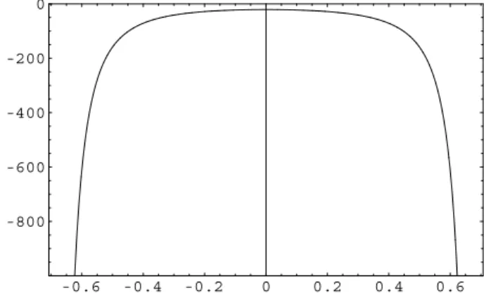
with mass m2v=−3k2¡7+25k2z2¢/¡
1−2k2z2¢2. The Fig. 1 shows the variation of m2
v with the extra co-ordinate. It is almost constant for small z and diverges for z→ ±z∗=±1/(√2k). On the |z|=0 3-brane, ˜Pµ(x) = cµe
13
4 tanh−1(1/3)eipαxαe−i58π, where p2=m2
v(0) =−21k2and, pµcµ=0.
Graviton. To obtain the graviton potential we take cµ=0 and Tµ(νm)=0. Then, the eq. (11) implies
[−∂2z+Vg(z)]ψg(z) =m2gψg(z), (20)
where Vg=−(32f′2−94f′′). This potential reproduces the RSII result for f(z) =Log(k|z|+1).
V. CONCLUSIONS
In the no warped scenario, the vacuum fluctuations are de-scribed by three independent wave equations which describes the 4D scalar, vector and tensor fluctuations on the|z|=0 3-brane. In warped scenarios, there are no scalar propagation on
-0.6 -0.4 -0.2 0 0.2 0.4 0.6
-800 -600 -400 -200 0
FIG. 1: The squared tachyonic mass, m2v(z), in the vertical axis. The horizontal axis is z∗≤z≤z∗and k=1.
the 3-brane vacuum. For the RS warp, there are no gravivec-tor on the 3-brane. For the smoothed warped braneworld, we obtain a tachyonic mass solution for the gravivector, that also satisfies the compatibility condition. This solution becomes a massless spin-1 fluctuation ifΛ5→0.
VI. ACKNOWLEDGEMENTS
I thank Dr. R. M. Marinho Jr. This work supported by brazilian agency CNPQ (gr. 150854/2003-0) and ITA.
[1] L. Randall and R. Sundrum, Rev. 83, 4690 (1999) [hep-th/9906064]; Ibd. 83, 3370 (1999) [hep-ph/9905221].
[2] J. Ponce de Leon, Grav. Cosmol. 8 (2002) 272-284. [gr-qc/0104008]; Int. J. Mod. Phys. D11, 1355 (2002)
[gr-qc/0105120].