Stochastic Molecular Dynamics of Colloidal Particles
Claudio Scherer
Instituto de F´ısica, Universidade Federal do Rio Grande do Sul, CEP 91501-970, Porto Alegre, RS, Brazil
Received on 2 September, 2003
Colloidal particles move in the carrier liquid under the action of several forces and torques. When the particles carry a dipole moment, electric or magnetic, as in ferrofluids, the rotational and translational motions are cou-pled because the field on a particle depends on the spatial and directional distribution of the others and the force and torque on it depends on the field. Moreover, there is Brownian, as well as dissipative forces and torques on each particle. Consequently, the numerical solution of the equations of motion requires, besides the techniques of Classical Molecular Dynamics, those of Stochastic Dynamics. The algorithm is explained in some detail and applied on a typical ferrofluid. For different values of the temperature, the possibility of the formation of structures is examined.
1
Introduction
Colloidal particles have translational and rotational mo-tion, due to several forces and torques. Besides forces and torques due to applied fields and inter-particle interactions, the molecules of the carrier liquid collide incessantly with the particle, causing translational and rotational Brownian motion. Their movement inside the liquid is opposed by viscous, dissipative, forces and torques. For simplicity, we will consider only spherical particles. We also assume that each particle carries a permanent dipole moment, which may be electric or magnetic. By using the appropriate Langevin equations we simulate realizations of the stochastic process which is the coupled motion of a sample of particles dur-ing a time which is sufficiently long for the thermodynamic equilibrium to be established. We use in the simulation typical values for the parameters, which correspond to re-alistic ferrofluids[1]. For recent references on ferrofluids, see the bookFerrofluids: Magnetically Controllable Fluids and Their Applications, edited by Stefan Odenbach[2]. Our procedure and results of the simulations are compared with those of Wang, Holm and Mller[3], recently published.
2
The Equations of Motion
The equations of motion for each particle can be written as one vector equation for its rotation around its center of mass and one vector equation for the translation of the center of mass. There is formally only one difference in the rotational equations of motion of colloidal particles having magnetic or electric dipole moments. This difference is in the exis-tence of an intrinsic angular momentum, S, associated to the magnetic momentµ,
µ=gS (1)
whereg is the gyromagnetic factor. There is no intrinsic angular momentum associated with electric dipoles. The ro-tational equation of motion for a solid particle is given by Classical Mechanics,
dJ
dt =N (2)
whereJ is the total angular momentum andN is the total torque. The magnetic particles of ferrofluids may be super-paramagnetic, when the magnetic moment is free to rotate with respect to the particle, or ”blocked”, when the magnetic moment is fixed in the particle. The case of superparamag-netic particles in ferrofluids has a more complicated dynam-ics because the magnetic moment and the particle’s Euler angles are independent, but interacting, variables[4, 5, 6]. In this work we consider only blocked magnetic particles. For spherical magnetic particles the angular momentum may be written as
J =Iω+S (3)
where I is the moment of inertia andω is the angular ve-locity. For electric dipolar particle the relation is the same, except thatS =0. The time derivative ofµis related toω, for blocked magnetic or electric dipoles, by
dµ
dt =ω×µ (4)
The torqueN has several origins. If there is a fieldF, which may be the magnetic inductionBor the electric field E, at the particle’s position, there is a torque
NF =µ×F.
by normalized white noise, with average zero and delta type correlation function,
ξ(t)= 0 (5)
ξi(t)ξj(t′)=δi,j δ(t−t′) (6) wherei,jindicate the Cartesian components.
The rotational motion is opposed by a dissipative torque, −λω, due to the liquid’s viscosityη, through the Stokes re-lation for rotation,
λ=πη d3
wheredis the diameter of the spherical particle. Einstein’s relation for the constants σ andλ and the temperature T
reads
σ=√2λkT (7) wherekis Boltzmann’s constant.
Summing up, we come to the following equation for the rotational motion,
Idω dt +
1
g dµ
dt =µ×F −λω+σξ (8)
which, together with Eq.(4), form, ifF is known, a com-plete set of equations for the vectorsω andµ. The same equations describe also electric dipolar particles, except that the second term at the LHS of Eq.(8) is absent. However, when particle-particle interaction is important, as we want to consider in this work,F is dependent on the particle po-sitionras well as on the other particles positions and mo-ments. Consequently, we have to solve simultaneously the rotational and translational equations of motion for all parti-cles.
The translational motion is described by Newton’s equa-tions,
dr
dt =v (9)
mdv
dt =f (10)
for the position vectorrand velocityv. The forcef on the particle, like the torque, has several origins. If there is a field gradient∇F at the particle’s position, then the force due to
this field is
fF =∇F ·µ. (11)
The particle-particle interactions are partly due to their contribution to the fieldF, but we also assume a hard core interaction which avoids two particles to come closer than a distancedbetween their centers. This is not contained in the expression forf, but will be introduced directly in the integration procedure. The stochastic force, due to the col-lisions of the liquid’s molecules with the particle, has the formαΓ(t), whereαis a constant andΓ(t)is also modeled by normalized white noise, like in Eqs. (5) and (6). There is
also a dissipative force−γvopposing the translational mo-tion. The dissipative constantγis related to the viscosity by the following Stokes relation,
γ= 3πηd. (12) Einstein’s relation for the constantsαandγand the tem-peratureT reads
α=2γkT (13) Summing up, we arrive at the following equation for the translational motion:
mdv
dt =∇F ·µ−γv+αΓ(t) (14)
which, together with Eq.(9), form a complete set of equa-tions for the variablesrandvifF(r, t)andµare known. However the particle-particle interactions makeF to depend on the magnetic moments and positions of all particles, so that simultaneous solutions of all equations of motion is nec-essary.
3
Numerical Solution of Langevin
Equations
Before discussing the procedures to solve the equations of motion of section 2, we present a brief introduction to nu-merical solutions of stochastic differential equations with white noise terms, known asLangevin equations.
Consider an n-dimensional stochastic processX(t), de-scribed by the following general Langevin equation,
dX
dt =A(X, t) +B(X, t)·ξ(t) (15)
whereA(X,t) is a well behaved n-dimensional vector func-tion,B is an n×m matrix and m is the number of inde-pendent components of the normalized white noiseξ(t). If Bdoes not depend onXwe say the noise isadditive, oth-erwise it is calledmultiplicative. For our present purpose it is not necessary to allow for explicit dependencies ofAand Bont, so thatA=A(X)andB =B(X)
It is impossible to simulate, in the computer, realizations of the white noise, since its correlation time is zero. There-fore we integrate formally Eq.(15) betweentandt+ ∆t,
∆X(t)≡X(t+ ∆t)−X(t) =
=
t+∆t
t
A(X(t′))dt′+ t+∆t
t
B(X(t′))·ξ(t′)dt′ (16) SinceAis a continuous function ofX, which is a con-tinuous function oft, we know, from the mean value theo-rem, that there is at least one valuet¯oft′such that the first integral above is
t+∆t
t
For the second integral at the RHS of Eq.(16) we con-sider first the case of additive noise. ThenBmay be taken outside the integral, so that the equation becomes
∆X(t) =A(X( ¯t))∆t+
+B·
t+∆t
t
ξ(t′)dt′ (18) The integral above is known asWiener increment,
∆W(t) =W(t+ ∆t)−W(t) (19)
where
W(t) =
t
0
ξ(t′)dt′ (20) is theWiener process.
The components of the Wiener increment∆W(t) are Gaussian stochastic processes with zero averages and stan-dard deviations equal√∆t. These properties of ∆W are fundamental for simulating realizations of the solutionX(t)
of Eq.(15).
Eq.(18) has then a form very appropriate for numerical simulation,
∆X(t) =A(X( ¯t))∆t+B·∆W(t) (21)
In numerical simulation∆t, in Eq.(21), is the length of the time step for integration. If we choose a very small∆t, X(¯t)may be substituted simply byX(t), or we may prefer a more precise algorithm, like Runge-Kutta second order. The components of∆W are generated, at each time step, as the product of√∆tby random Gaussian numbers with zero average and unit variance.
The case of multiplicative noise is more complex. The rigorous treatments of Ito and of Stratonovich give us the prescriptions to follow, which are equivalent in the limit
∆t →0, but for finite∆tthey have different speed of con-vergence to the exact result. According to my own experi-ence, by treating several examples, the Stratonovich proce-dure converges more rapidly than that of Ito, but, in many cases, it is more difficult to implement. We use here the Stratonovich procedure, according to which the equation equivalent to Eq.(21) for multiplicative noise should be writ-ten as
∆X(t) =A(X( ¯t))∆t+B
X(t) +∆X(t) 2
·∆W(t)
(22) When we can isolate∆X(t)in Eq.(22), very good, other-wise we may, for example, use simplyB(X(t))to obtain a first approximation for∆X(t)and then substitute this value in the RHS of the Equation.
4
Numerical Simulation on
Ferroflu-ids
Initially we consider the orders of magnitude of the terms in Eqs. (8) and (14). We start with the simplest one, which is
Eq.(14). Applying the procedure described in section 3 to the system of Eqs. (9) and (14), follows
r(t+ ∆t) =r(t) +v¯(t) ∆t (23) and
v(t+ ∆t) =v(t) + 1
m(∇F·µ−γv¯(t))∆t+ α
m∆W(t)
(24) An alternative approximation to those equations consists in neglecting the inertia term in Eq.(14), which leads to
r(t+ ∆t) =r(t) +1
γ∇F ·µ∆t+ α
γ∆W(t) (25)
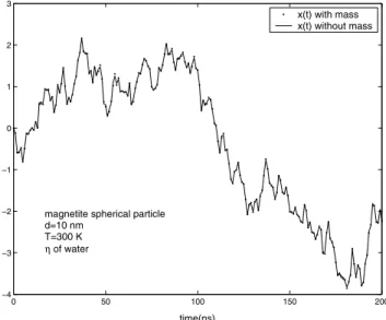
The numerical simulation of the system of Eqs. (23) and (24) and of Eq.(25) was made for the same realization of W(t), with∇F = 0. As parameters we used those of a
magnetite spherical particle of diameterd=10 nm in a liquid whose viscosity is that of water, atT=300 K. The results for one component ofr(t)are shown in Fig. 1. We see that the effect of taking into account the mass is, indeed, negligible. This conclusion becomes even more evident in Fig. 2, where we used for the mass a value 100 times bigger, keeping the other parameters unchanged.
0 50 100 150 200
−4 −3 −2 −1 0 1 2 3
time(ns)
x(t) with mass x(t) without mass
magnetite spherical particle d=10 nm T=300 K
η of water
Figure 1. Translational motion of a magnetite particle, with the standard parameters given on the text.
The advantage of neglecting the mass is that the conver-gence to the limit ∆t → 0 is much faster than when the mass term is present, which makes an important difference in CPU time when we simulate a system of many interacting particles.
0 50 100 150 200 −4
−3 −2 −1 0 1 2 3
time(ns)
x(t) with mass 100 × bigger x(t) without mass
Figure 2. Translational motion of a particle; the dotted line cor-responds to a particle with a fictitious mass 100 times bigger than that of our standard magnetite particle
1) Neglecting I:
Let us define the following symbols:
s =µ/µ0, whereµ0 =|µ|is a constant for blocked
mag-netic moment;∆W⊥= ∆W −s(s·∆W)is the compo-nent of∆W perpendicular tos. After some vector algebra we get, neglecting terms of order higher than∆t2
,
∆s=A−1
·(g(s×F) ∆t+ ¯σ∆W⊥) (26) where
A=
1 −¯λ sz ¯λ sy
¯
λ sz 1 −λ s¯ x −¯λ sy λ s¯ x 1
(27) beingsx, sy, szthe Cartesian components ofs,λ¯=g λ/µ0
andσ¯=g σ/µ0. Finally,
s(t+ ∆t) =s+ ∆s. (28) We improve the quality of the simulation by renormalizing safter each integration step, making|s|= 1.
2) Neglecting the intrinsic angular momentum S =
µ/g:
Again, after some algebra and neglecting terms of order higher than∆t2, we come to the set of equations
∆ω=µ0(s×F)∆t−λω∆t+σ∆W
I(1 +λ∆t/2) (29) ¯
ω=ω+∆ω
2 (30)
and
∆s= (ω¯×s)∆t (31)
The procedure is then simple: for given ω(t),s(t),F(t) and ∆W we calculate ∆ω,ω¯ and ∆s in this order, and then ω(t + ∆t) = ω(t) + ∆ω and s(t+ ∆t) =s(t) + ∆s.
3) Neglecting both,IandS:
In this case Eq.(8) becomes
µ×F −λω+σξ= 0 (32)
It takes again some vector algebra and the use of equation
ds
dt =ω×s (33)
to transform Eq.(32) to the form
ds
dt = µ0
λF⊥+ σ
λξ×s (34)
where
F⊥=F −s(s·F) (35)
The corresponding discretized Langevin equation is
∆s= µ0
λF⊥∆t− σ
λs×∆W (36)
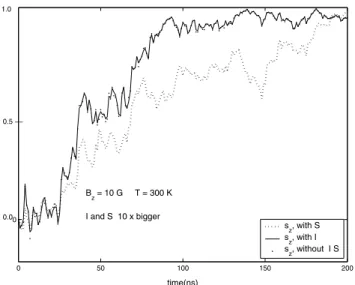
In Fig. 3 we show sz(t) obtained with the three ap-proaches just described, for the same realization ofW(t), using the parameters of a realistic magnetic particle in a fer-rofluid: a spherical magnetite particle with diameter of 10 nm in a liquid with the viscosity of water at room tempera-ture and in presence of a weak magnetic field of 10 G.
We see that taking into account the moment of inertia,
I, or the intrinsic angular momentum,S, has practically no effect on the result of the simulation. To enlarge the effect of those terms we repeat the simulation with fictitious values of
IandS10 times bigger than those of the standard magnetite particle of 10 nm in diameter, keeping the other parameters unaltered. The result is shown in Fig. 4. In this caseShas a considerable effect butI is still absolutely irrelevant, so that, if one of those terms should be taken into account, that should beSand notI. The opposite procedure was made in reference [3], as mentioned in our introduction.
0 50 100 150 200
0
time(ns) s
z, with S
s
z, with I
s
z, without I S
B
z=10 G
T = 300 K
0.5 −− 1.0
0 50 100 150 200 0
time(ns)
s
z, with S
sz, with I s
z, without I S
B
z = 10 G T = 300 K
I and S 10 x bigger
1.0
0.5 −−
0.0
Figure 4. Same as Fig.3, but for a fictitious particle with I and S 10 times bigger than that of our standard magnetite particle.
5
The
Inter-particle
Forces
and
Torques
The forces between the magnetic particles in a ferrofluid are of two different origins: 1) A short range repulsion, which avoids two particles to overlap in space and 2) magnetic dipole-dipole force. The first we simulate by a hard spheri-cal core with the size of the particle; the dipolar force on a given particle is calculated in the following way: we calcu-late the field gradient∇B, whereBis the magnetic
induc-tion on the particle’s posiinduc-tion due to the other particles in the sample, then
fp=∇B·µp (37)
whereµpis the particle’s magnetic moment.
For a particle at positionrp, the magnetic induction due
to the other particles is
B(rp) = j=p
3n(µj ·n)−µj
|rp−rj|3
(38)
wherenis a unit vector in the direction ofrp−rj. The torque onµpis
Np=µp×B(rp) (39)
−2 0 2 4 6 8 10 12 14 16
−2 0 2 4 6 8 10 12 14 16
Periodic Boundary Conditions
p
1
2 2
3 3
4 4
5
5
Figure 5. A two-dimensional sketch of our procedure for periodic boundary condition.
The numerical simulations on a random homogeneous distribution of magnetic dipoles have convinced us that the contribution to B(rp) due to the dipoles which are more than a few inter-particle distances apart fromrp is totally negligible. This is so because when the spacial distribution of the moments is precisely homogeneous, even if there is a preferential direction for their orientation, the field at the center of a cube, due to the other particles in the cube, is zero. Therefore a non zero field comes only from deviations from homogeneity, which is really important only in short distances. Our simulation is done on a cubic box of side
L of a ferrofluid containing 1000 magnetic particles. We use periodic boundary conditions. To calculate the induc-tion B atrp due to the particle atrj, if the x-coordinate
xp−xj > L/2we substitutexj byxj+Lin Eq.(38), and similarly for the other coordinates; ifxp−xj <−L/2we substitutexj byxj −L. With this procedure, the field on each particles considers all other particles which are in the cube of sideLof which the considered particle is at the cen-ter, as is indicated in a two-dimensional projection in Fig. 5. To calculate the field on particle p in Fig. 5, due to all other particles inside the simulation box, in solid line, we use, in the case of particle 1, its actual coordinates but in the cases of particles 2, 3, 4 and 5, the coordinates of their periodic images, which are inside the box in doted line, of which p is the center.
After each integration step we translate each particle which went out of the simulation box like particle 2 in the figure, to inside the box, at the position of its periodic image. We start the simulation by placing the magnetic particles at the sites of a cubic lattice inside the simulation box, the components of the magnetic moments are chosen at random and the modulus normalized toµ0. The fields and field
signifi-cantly anymore, the resulting distribution is shown in Fig. 6 for a slice of the simulation box, parallel to the x-y plane and of width equal to the average inter-particle distance. In Fig. 6 the lines indicate the projection of the magnetic mo-ments on the x-y plane. We see that nothing of the lines of aligned dipoles, as reported in reference [3], can be seen. On the other hand, simulation made on a fictitious ferrofluid at T=3K (not 300K) lead to Fig. 7, where lines similar to those reported in reference [3] are seen. This result makes us sus-pect that an error in the generation of the noise was made by the authors of reference [3], resulting in noise terms much weaker than what should be the case at 300 K.
0 50 100 150 200
0 20 40 60 80 100 120 140 160 180 200
Figure 6. A slice of the simulation box at the end of the simulation for T=300 K, showing the magnetic particles and their magnetic moments(lines) normalized to one and projected on the x-y plane.
0 50 100 150 200
0 20 40 60 80 100 120 140 160 180 200
Figure 7. Same as in Fig.6, but for a fictitious ferrofluid at T=3 K.
References
[1] R.E. Rosensweig,Ferrohydrodynamics, Dover Publications, Inc., New York, 1997.
[2] S. Odenbach (Ed.), Ferrofluids: Magnetically Control-lable Fluids and Their Applications, Springer-Verlag, Berlin (2002).
[3] Z. Wang, C. Holm, and H.W. M¨uller, Phys. Rev. E66, 021405 (2002).
[4] M.I. Shliomis and V.I. Stepanov, Adv. Chem. Phys. Series87, 1 (1994).
[5] C. Scherer and G. Matuttis, Phys. Rev. E63, 011504 (2001).