doi: 10.1590/0101-7438.2014.034.02.0319
INVESTORS’ ASYMMETRIC VIEWS AND THEIR DECISION TO ENTER BRAZIL’S WIND ENERGY SECTOR
Marta Corrˆea Dalbem
1*, Leonardo Lima Gomes
2and Luiz Eduardo Teixeira Brand˜ao
2Received January 16, 2013 / Accepted March 9, 2014
ABSTRACT.Market players’ investment decisions sometimes surprise analysts, especially when projects that are less feasible in financial terms enter first in the market, before more viable projects. One possible explanation is that firms have different expectations concerning the future of the market. In this article we use the Option-Games approach for asymmetric duopolies to analyze investors’ decisions in the first auction for wind power in Brazil, held in 2009, in which some less viable firms pushed more viable firms out of the auction. Our analysis shows that even small differences in the investors’ views can yield this unexpected result. When uncertainty is low and expectations are symmetric, the outcome is a lower energy tariff as well as a stronger wind industry in Brazil, highlighting the importance of a clear and credible long term governmental policy, not only for the wind industry, but also for any other industry in its early stages.
Keywords: investment decisions, Option-Games, Real Options.
1 INTRODUCTION
Wind power has grown on average 24% per year worldwide in the past decade, reaching 254 GW of installed capacity by mid 2012, with China, USA, Germany, Spain and India accounting for 74% of this total (WWEA, 2012).
With 84% of its power capacity based on renewable sources and mostly self sufficient in energy, Brazil has been a late entrant into the wind power industry with 2.0 GW in installed wind energy capacity, most of which was fostered by the Proinfa feed-in incentive program for renewable sources. Nonetheless, Proinfa wind farms faced delays in beginning operations, reflecting a dif-ficult learning curve which coupled with the higher tariffs for this energy source, reduced the government’s interest in fostering new wind farms during the 2005-2009 period.
*Corresponding author
Despite this slow start, wind energy is a viable alternative to contain the increasing carbonization of Brazil’s power system, especially considering that the most viable hydro resources have al-ready been explored. Therefore, in December of 2009 the Brazilian government opted to contract new wind farms through a reverse auction. To some surprise, the offer of energy in this auction was three times greater than the demand while prices dropped 22%. Six other auctions were held in 2010-2012, two of them following the same set of rules of the 2009 auction and the remainder based on different rules, signaling that the Brazilian energy regulatory agency is still testing the best way to foster wind energy.
We analyze the results of the first wind energy auction held in 2009, a time when short term energy prices were trading at the R$ 16.5/MWh floor (USD 9.4/MWh), which led some players to believe that the government would not contract a significant amount of more expensive wind energy in the forthcoming auctions. In addition, Brazil’s 10-yr Plan for the Expansion of Energy Supply forecasted that wind energy would represent only 1% of installed capacity in 2017. On the other hand, delays in the construction of thermal and hydro plants indicated that wind energy might be a good alternative to meet the 52% growth in demand forecasted for the 2008-2017 period. Market players had, therefore, reasons to have different expectations of the future for wind energy in Brazil.
Would it be better to invest as soon as possible, or rather wait for a clearer market perspective? Waiting to invest has an opportunity cost, as competitors gain market share and push costs up, while investing immediately would mean incurring in high initial costs in order to establish a foothold in a still uncertain market and accept lower margins, in order to win a very competitive auction.
The outcome of the 2009 auction was surprising as newcomers with projects in sites with lower wind potential won, while some more traditional firms with worldwide experience in the industry did not even place bids. Oddly enough, the firms that abandoned the 2009 auction did take part in the following auctions held in 2010 and 2011, selling their energy at much lower prices than those they had considered unacceptable in the 2009 auction, signaling once again that they have always had an interest in establishing a foothold in Brazil and postponed entry for other reasons. One of the reasons might be their subjective view of this market’s perspectives.
We develop an Option-Games model to attempt to explain this behavior and analyze what might have induced entrepreneurs with projects that are, at first glance, less feasible, to be more aggres-sive at the auction and enter the market first.
This paper is organized as follows. In Section 2 we present a review of the literature on Option-Games and the intuition behind duopoly games and in Section 3 we detail the assumptions for the model of duopoly games in the presence of three asymmetries which was adopted. In Section 4 we apply this model to a practical case and discuss the results of a sensitivity analysis and in Section 5 we conclude with policy recommendations that may be useful for both investors and governments.
2 LITERATURE REVIEW
Traditionally, the corporate capital budgeting decision is based on the Discounted Cash-Flow Method (DCF), in which the myriad of possible future scenarios are represented by the expected scenario. This method, however, does not take into account the fact that managers have the flexibility to make optimal decisions in the light of new information that may be revealed over the life of the project, and that such flexibility may add significant value to the project.
Tourinho (1979) used financial option theory, based on the seminal works of Black, Scholes (1973) and Merton (1973), as an inspiration to value a project with embedded options subject to uncertainty. This pioneering work marked the beginning of the literature field that is now known as Real Options Analysis (ROA), and which was further consolidated by the contributions of Brennan & Schwartz (1985), McDonald & Siegel (1986), Trigeorgis (1993), Copeland & Antikarov (2003) and Brand˜ao, Dyer & Hahn (2005).
In Brazil, Real Options literature is growing, with theoretical contributions and also empirical works such as Novaes & Souza (2005), regarding options to expand capacity, and Rocha et al. (2007), which analyze the opportunity to make sequential investments, but in the Real Estate market. Local literature on Real Options also include several works in the energy sector: Gomes & Luiz (2009) value the flexibility inherent to negotiations in the Brazilian free market for en-ergy; Fenolio & Minardi (2009) value small hydro-power plants; Bastian-Pinto, Brand˜ao & Hahn (2009) value ethanol plants; Batista et al. (2011) analyze the value of the option to sell carbon credits, for an energy generator; Dias et al. (2011) value the options in a cogeneration project of a sugar/ethanol plant. However, there is not, as yet, relevant production involving wind energy and/or energy auctions, using Real Options.
Huisman & Kort (2001) extend Smets’ model to the analysis of players that already operate in the market, while Huisman & Nielsen (2001) analyze a duopoly in which players are asymmetric in terms of the initial investment. Pawlina & Kort (2006) extend Huisman & Nielsen’s work by improving the analysis of the market conditions under which players have an incentive to invest simultaneously. Smit & Ankum (1993) and Smit & Trigeorgis (2004) focus on discrete time models for option-game theory, while Azevedo & Paxson (2010) provide a thorough revision of the literature and show that this field is still undeveloped. In Brazil, game theory has been applied to the energy and oil sector, as in the work of Pompermayer et al. (2007), but the bridge between Real Options and Game Theory has not, as yet, been developed.
In this article we use the works of Huisman & Nielsen (2001) and Pawlina & Kort (2006) regard-ing preemption games and asymmetric duopolies as theoretical references and extend them to the case where players have three asymmetries. The third asymmetry involves the players’ sub-jective view about the market’s future, as reflected in differentiated diffusion processes to de-scribe the market uncertainty. To the best of our knowledge, this represents an original contribu-tion to the literature.
By adopting a preemption game we are actually performing an analysis of one group ofn-players that, despite being economically more feasible, loses an energy auction to a second group ofm -players that are economically less feasible. This analytic simplification is equivalent to say that each of the two groups is represented, in our duopoly preemption game, by a characteristic firm.
In preemption games, each firm decides in favor of the alternative with the best balance between the advantages of investing earlier (preempting the market and becoming the Leader) and the advantages of waiting to invest. Investing earlier protects the profitability of the Leader’s projects when there are first-mover advantages; on the other hand, the Follower keeps the flexibility to invest at hopefully more favorable conditions. Each players’ optimal strategy will depend, however, on what they expect will be the competitor’s rational response to the market conditions. This is equivalent to an “optimal stopping” problem: each player analyzes when it is optimal to stop waiting and finally make the decision to enter the market, but also takes into account the competitor’s best response.
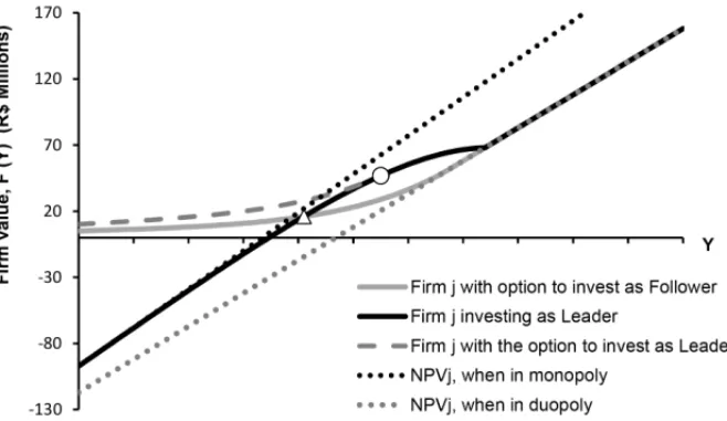
Figures 1, 2 and 3 provide some intuition behind Option-Games models for duopolies. The upper straight dotted lines in Figure 1 shows the Net Present Value of a monopolistic firm (the firm’s N PV is noted here asF) as a function of a state variableY, a stochastic variable that may reflect, for example, the combined effect of changes in wind energy prices and equipment costs on the value of the firm’s standard wind farm. As a second firm enters the market, prices tend to drop due to more firms interested in bidding in future auctions, and/or increasing construction costs due to a higher demand for equipment, which make the firm’s valueF drop to the lower dotted line.
70 120 170
F (Y),
(R$
M
il
li
ons
)
Ͳ130
Ͳ80
Ͳ30 20
F
irm
v
a
lu
e
,
Y
Firm j investing as Leader
NPVj, when in monopoly
NPVj when in duopoly
NPVj=Firmj'sNetPresentValue =F(Y)
Figure 1– The Leader’s value curve.
Figure 1, which reflects the duopoly case. For realizations ofY between those two extremes, the firm’s value grows slower withY, reflecting the ever higher chances that the competitor will also enter the market, making the Leader face tougher market conditions. Therefore, the Leader’s value curve has the shape depicted in the dark continuous line in Figure 1, and it touches the duopoly straight line when Y reaches the value that finally attracts the opponent to enter the market as the Follower.
On the other hand, if this firm were in the position of Follower, its value while still holding the option to enter the market as Follower is represented by the continuous grey line in Figure 2.
For realizations ofY beyond the triangular point depicted in Figure 2, the firm’s value as Leader is superior to its value as Follower; therefore, there is already an incentive to enter the market as the Leader – this is the firm’s preemption region. However, the firm will not necessarily do that immediately: if there is no threat that the competitor will preempt the market, the firm may still wait for better market conditions or, in other words, the option to wait is still more valuable than investing immediately. If such is the case, the firm will only enter the market as Leader in the circular point illustrated in Figure 2. Leahy (1993) demonstrates that this is also the entry point of a firm in a monopoly condition, using the Real Options rationale.
Figure 3 shows the value curves of two firms in a duopoly that are asymmetric in terms of the initial investment needed to enter the market. This asymmetry is reflected on the different points at which the value curves intersect the vertical axis. When the two firms are also asymmetric in terms of their yearly future cash-flows, the dotted value lines are also not parallel. The value curves related to the more viable firm are shown thicker, while the less feasible firm is repre-sented by a thinner line. The dark square points mark the moment when the two firms actually enter the market, which is the solution to the game.
Figure 3– Value curves for two firms in duopoly and the entry triggers (squared points).
3 A THREE ASYMMETRY OPTION-GAME MODEL
Wind energy auctions in Brazil are in descending format with starting ceiling prices that are set by the government. The price is steadily reduced by a fixed amount or percentage previously informed to bidders, who abandon the electronic auction when the price drops below their min-imum established level. In our Option-Game model, abandoning the auction is equivalent to deciding to wait for a better opportunity, or equivalently, to deciding not to exercise the option to invest.
Bidders are unaware of how much energy the government intends to contract and the number of players that are still competing at any time. The auction is interrupted by the government when the offer of energy is still above the demand, based on criteria known only to the government. Next, the previous bid’s results are reinstated and the remaining players are called upon to input their last sealed-bid into the system. The government then contracts enough projects to meet demand, from the lowest to the highest prices. Winners commit to deliver energy for 20 years beginning three years from the date of the auction, which is the time required to build the new wind farms, and at the prices fixed at the auction plus inflation.
13 14
10 11 12
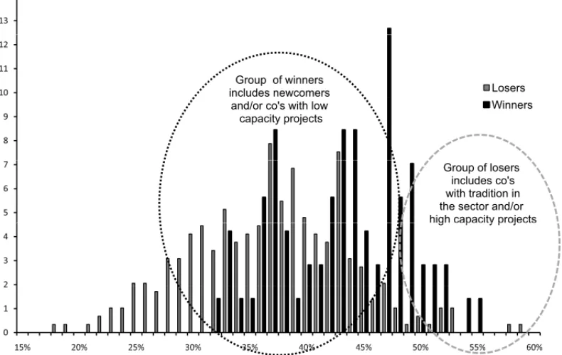
Losers Group of winners
includes newcomers
8 9
Winners and/or co's with low
capacity projects
5 6
7 Group of losers
includes co's with tradition in the sector and/or high capacity projects
2 3 4
g capac y p ojec s
0 1 2
15% 20% 25% 30% 35% 40% 45% 50% 55% 60%
15% 20% 25% 30% 35% 40% 45% 50% 55% 60%
Figure 4– Results of the 2009 wind energy auction in Brazil: Nr of bidders×Expected Project Capacity Factor (%).
incentives, wind potential, all of them translating into a lower capital expenditure (CAPEX) to produce the same amount of energy, for illustration purposes we single out the firm’s project capacity factor as an indicator of its economic feasibility in Figure 4.
We assume that these two groups can be represented by two characteristic firms confronted with the decision to enter or not in the market. The problem is therefore reduced to an asymmetric duopoly in a preemption game, in which the decision to enter the market is equivalent to accept-ing the interval of energy prices that were contracted in the 2009 auction.
We also assume that the decision to enter the market represents, in fact, a long term commitment to grow in the industry, that is, the firm will steadily build a portfolio of standard wind farms in the same region, adding one standard farm per year. Having decided to enter the market, the player will reap a stochastic payoff that will depend on the future price and cost conditions of the wind market. The value of each firm will be, therefore, the sum of the stochastic net present values of the standard wind farms the firm will steadily aggregate to its portfolio. We note the standard wind farm’s stochastic value as V (= N PV of the firm’s standard project) and each standard wind farm is assumed to produce and sell 25MW on average.
The firms in the duopoly are asymmetric in terms of the initial investment to establish a foothold in the market, the value of their standard wind farms and their views about the market prospects. Our game is non-cooperative and sequential (Stackelberg,apudGibbons, 1992) and each of the two firms holds an American option to enter the Brazilian wind market, meaning that they can enter the market anytime.
Our model assumes that the demand for energy grows organically in a way that the output of one new standard wind farm can be absorbed by the market without causing impacts either on energy prices or on the sector’s costs. However, when both firms are already in the market, each aggregating one new standard wind farm per year, the competitive pressure pushes the market to a new and unfavorable condition, described by an inverse demand function(D), deterministic, so that theVsdrop in value.
In addition, the project valueV is affected by uncertainties related to the overall energy market, the economic environment, the cost of industrial commodities, and so on; those uncertainties are included in the model by means of a stochastic shock Y˜, so that the value of the Firmi’s standard project,Vi, is stated as: V˜i = ˜YiDi N i,N j, noting thatDi N i,N j is a deterministic value that drops when there is more than one firm in the market – and therefore a higher energy offer in the market. The valueViof each new standard wind farm aggregated to Firmi’s portfolio varies not only withDi N i,N j, but also with a stochastic variable(Y˜i), which we assume follows a GBM (Geometric Brownian Motion) diffusion process shown in Equation 1.
dYi =αiYidt+σiYid zi (1)
whereαireflects the drift (the expected trend forY),σiis the standard deviation (a proxy for what Firmi forecasts to be the uncertainty in this market), and the random incrementd zi =ξ
Given thatDis deterministic,V˜ifollows the same stochastic process asY˜i.
The GBM assumption is due to the fact that V is affected by a number of factors that impair any attempt to infer what would be a long term equilibrium level. For example, wind energy is a new market, still far from the stable conditions of other more mature industries. In a GBM diffusion process, the drift term a dominates the behavior ofV in the long run, while the short term behavior is more influenced by the volatility parameter (Dixit & Pindyck, 1994, p. 67), which agrees with the intuition on the behavior ofV. The lognormal assumption of the GBM also does not allow for negativeVs. This automatically adjusts our model to the fact that the firms will only aggregate new wind farms to the portfolio if they have a positive net present value, which is consistent with reality.
The deterministic term, Di N i,N j, reflects the inverse demand function applicable to Firmi and depends only on the condition of the players in the duopoly, hereby described by the subscripts N i and N j. N i is zero when Firmi has not entered the market yet, while it is equal to 1 if Firmihas already invested. The same rule applies toN j.
Di10→ deterministic component of theV of Firmi when it has already entered the market as Leader, while Firmj has not entered yet
Di11→ deterministic component of theV of Firmiwhen both firms have already entered the market
In our model,Di10 >Di11in order to reflect that the firm reaps a higherV iwhen it is alone in the market; when the competitor also enters the market, the Leader’s futureVs tend to drop. The function that describes theV of Firm j is similar to that of Firmi, but with different parameters for the stochastic process:V˜j = ˜YjDj N i,N j, whereDj01>Dj11and
dYj =αjYjdt+σjYjd zj. (2)
The deterministic components of Firmi’s V are smaller than those of Firm j, Di10 < Dj01;
Di11 < Dj11. This is the first asymmetry in our problem, which can be translated as Firmi being less economically viable than Firm j, simply because it owns standard farms with lower valuesV. We assume that the size/experience of each firm’s shareholders, as well as the fore-casted capacity factor and location of their wind farms, are good indicators of the value of each player’s first wind farm. This information is disclosed to the bidders in the Brazilian wind energy auctions.
The second asymmetry, also known to the players, refers to the initial investment,I, necessary to establish a foothold in the market. This investment refers to hiring bonuses, acquiring knowledge about wind potential (measurements of wind behavior), consulting services, costs to open a new firm, legal costs, soIi >Ij, for the same reasons.
asymmetry in our problem. A player who adopts a positive drift is assuming that wind energy prices will increase in the next auctions or that equipment costs will drop, for example, while a higher volatility reflects a higher uncertainty over future market conditions.
This third asymmetry would make the problem become a game with incomplete information and infinite sets of expectations. We choose to restrict our analysis to two scenarios:
1) Model 1: Each player knows that the opponent has a different expectation of the future and knows what this expectation is;
2) Model 2: Each player believes there is no asymmetry in expectations and assumes the opponent shares the same expectations about the future (but it does not). This simplifica-tion resembles Schelling’s (1960) concept of focal point: informasimplifica-tion widespread in the market and/or each player’s own system of expectations help restrict the scenarios and the outcomes.
We assume that the initial realization ofY(Y0)is low enough to prevent both players from invest-ing immediately. A lowY0means that a firm’sV att =0 is close to zero. WhenY0is sufficiently high to stimulate both firms to invest, mixed-strategies equilibriums may occur, as well as simul-taneous investment. We disregard these possibilities as our objective is to identify which firm is tempted to invest first and at what energy price.
We also compare the results of Model 1 and Model 2 with those of a base case scenario in which there is no asymmetry in the players’ expectations about the future. The market tends to this base case when the government sends clear and reliable signals about the future demand for wind energy.
In Models 1 and 2, we developed the value functions for the two firms, similar to those illustrated in Figure 3, and for the following situations:
a) Firmi is the Leader and Firm j is the Follower;
b) Firm jis the Leader and Firmi is the Follower.
The problem is solved by backward induction, first determining the value function of the Fol-lower and subsequently the value function of the Leader, since the Leader’s decision to enter the market will be based on its expectation of when the opponent will optimally enter the market. The procedure for determining the value curves is detailed in Appendix A.
4 MODEL APPLICATION
4.1 Base Case Assumptions
and USD 2325/kW, which implies an asymmetry of 2%. The initial investment required to es-tablish a foothold in the market ofIi =R$ 13.20M andIj =R$ 12M reflects an asymmetry of 10% and will allow both to build and operate up to five standard wind farms in 5 years. These characteristics are typical of the Brazilian wind energy industry and are based on technical liter-ature of the industry and publicly available data disclosed by the Brazilian government’s energy research institution EPE –Empresa de Pesquisa Energ´etica. The assumptions are also in line with common sense, that is, traditional firms with worldwide experience enjoy a stronger bar-gaining power with equipment suppliers and do not need to offer premium wages in order to attract specialized personnel. In the wind industry, operating costs are irrelevant when compared to CAPEX and the initial investmentsIto organize the company, so these two values are the core reasons for the cost competitive asymmetry between Firmiand Firm j.
Projecting the free cash-flows of each firm’s first wind farm over its 20-year life and assuming an energy price of R$ 153/MWh (the highest price contracted at the 2009 auction), we obtained the expectedV0for the two firms in the duopoly. The cash-flows were discounted to their present values at a real interest rate of 10% per year, and the resultingVs– R$ 18.8M and R$ 22.0M – were used to estimate the parametersDi10andDj01, respectively.
We assumed an erosion of R$ 10M in the firms’Dswhen the competitor also enters the market, so thatDi11 =8.8 andDj11 =12. This R$ 10M erosion in value might occur, for example, if equipment costs grows by 6.2-6.4% or if energy prices drop to R$ 147.55-147.35/MWh ( < 4%) as a result of increased competition.
With this set of parameters, if the market for wind energy deteriorates to the extent that it be-comes unfeasible to add new wind farms to the portfolio, the values of the two firms would be Fi =8.8-13.2=(R$ 4.4M) and Fj =12.0-12.0=R$ 0M. Therefore, we adopted parameters which, while still consistent with the industry practice, make only Firm jeconomically viable in the scenario where both firms are already in the market. Firm jis also more robust to face other risks, such as the risk of wind variability.
TheVsof both firms are very sensitive to the main variables of the projected cash-flow: a 2% increase in CAPEX causes a 14% reduction inVs; a 5% increase in CAPEX causes a reduction of 35%. Likewise, a R$ 1/MWh reduction in energy prices causes a reduction in the Vs of R$ 1.37M, meaning that if energy price drops by 2%, from R$ 153/MWh to R$ 150/MWh for example, theV of Firm j will fall by 19%. So, the volatility to be adopted in the stochastic process of theVsmust be high and was initially arbitrated at 40% in the base case. For the same reasons, it is also reasonable that the parametersαi andαj, which mimic the firms’ expectation of growth or reduction in theVsbe high, so they were initially set at 5%.
The model applies the value functions specified in Appendix A to identify which realizations of Y trigger the entry of Firmi and Firm j in the market(Y i∗,Y j∗), for each set of parameters used in the sensitivity analysis. Such values ofY∗can then be translated into the firms’ V s∗ that trigger the entry (e.g.: V of Firm j as Follower: V j∗=Y j∗D j11;V of Firm j as Leader:
The triggerV∗for each firm generated by the model is then converted into a trigger energy price in R$/MWh, based on the deterministic cash-flow of the standard wind farm of each firm. This synthetic trigger-price is, in other words, the wind energy price that would make that firm’s first V be high enough to make the firm enter the market. If this falls within the prices that were contracted at the auction, this implies that this firm remained in the auction till the end and won the bid.
4.2 Results: Base case
With the set of assumptions detailed in Section 4.1, Firm jwould enter as Leader in the market, selling energy at R$ 143.64/MWh (Y =0.419). Firmi would be the Follower, entering the market in future auctions when energy price reaches R$ 154.02 (Y =1.152). The base case depicted in Figure 5 is consistent with the bids observed in the 2009 wind energy auction (R$ 131 – 189/MWh) and also reflects the situation in which only the more viable player, Firm j, would have sold energy at that auction, since the highest contracted price was R$ 153/MWh.
Figure 5– Value curves in the base case.
4.3 Results: Model 1
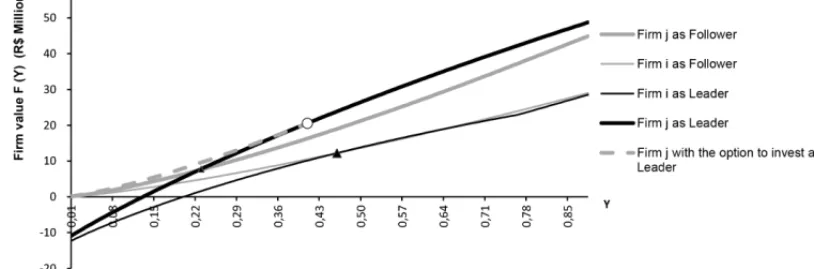
Figures 6 and 7 show what happens when we add asymmetry in the firms’ expectations about the future of the wind market. In Figure 6, Firm j believes the market will be more volatile (σi = 40%; σj = 55%). Assuming the competitor is more secure about the future, Firm j imagines the other player will soon be encouraged to also enter the market, preventing Firm j from reaping the first-mover advantages for sufficient time. Therefore, the less viable Firmi is the one to enter the market as Leader at Y = 0.3449, immediately before Firm j would also be encouraged to preempt the market. After all, the firms enter the market at price i = R$ 143.89/MWh and price j =R$ 153.53/MWh, that is, Firmi would have won the auction.
Figure 6–σi =40%;σj=55%.
Figure 7–αi =–29%;αj =5%.
on the other hand, forecasts a 5% yearly growth in theVs. In this case, Firmi enters as Leader atY =0.2799, just before the opponent’s preemption trigger (Y =0.280). As a result, the firms enter the market at pricei=R$ 143.00/MWh and price j =R$ 150.98/MWh.
Figure 7 shows that the value of Firmi as the Leader decreases for values of Y above 0.60. This happens under specific assumptions, such as the ones adopted in Figure 7, because higher values ofY increase the chances that the Follower will also enter the market soon, bringing in tougher market conditions – lower prices and/or higher implementation costs, the latter caused by competition for scarce resources such as land, specialized workers, and so on. When the Leader is not optimistic about the future and also has a less feasible project, the expected value erosion caused by earlier competition may more than compensate the expected gains from a higherY.
enters as Leader. This happens because Firmi faces a “now or never” decision: there is still a risk that the opponent will preempt the market imposing pressures on costs and revenues, while Firmi does not expect the market to improve soon enough to make waiting worthy. As a result, Firmiopts to enter first in the market, pushing the more viable Firmjto the position of Follower. In the pessimistic perspective of Firmi, the realization ofY that would trigger the opponent’s entry in the market would take long to happen, so it would be able to reap the first-mover advan-tages for a prolonged period of time, enough to make investments worthy immediately.
Figure 8 shows what happens when it is Firm j which believes that, on average, the future market conditions for wind energy will deteriorate. In such case, Firm j enters the market as Leader at Y =0.234, its trigger when in monopoly. The firms enter the market at price j = R$ 140.66/MWh and price i =R$ 154.02/MWh. The model is not sensitive to a pessimistic view of Firm j, that is, the decision does not change; this happens for any low or negativeαj because we adopted parameters that make Firm j already viable with just one wind farm in the portfolio. On the other hand, as described before, the decision changes when the less viable Firmiis the one with a pessimistic view, that is, Firmitends to preempt the market.
Figure 8–αi =5%;αj =–5%.
4.4 Results: Model 2
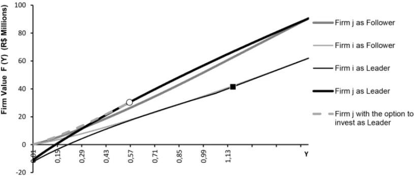
Figure 9 shows the value functions when the parameters are the same as those shown in Fig-ure 6, but now, although both firms still make decisions based on what they expect will be the opponent’s best response, their analyses are unfortunately based on incorrect assumptions on the other player’s expectations. In this situation of misinformation, Firm i does not preempt the market. Firm j enters first atY =0.577, its trigger as a monopolist, while Firmi enters as Follower atY =1.152. In summary, entry prices are: pricei =R$ 154.02/MWh and price
j=R$ 146.20/MWh.
Figure 9– Model 2,σi =40%;σj=55%.
mover condition, pushing it to enter as Leader atY =0.577, equivalent to R$ 146.20/MWh; if it had known the opponent’s correct stochastic process, Firm j would have invested only as Follower and atY =1.059, equivalent to R$ 153.53/MWh.
Firmi, on the other hand, imagines the opponent also believes the market will be less volatile in the future and, knowing it has projects with higherVs, assumes it will invest early, atY =0.419 or R$ 143.64/MWh. In this case, it is never optimal for Firmito invest as Leader. However, it plans to invest atY =1.152, at R$ 154.02/MWh, earlier, therefore, than expected by Firm j. As a result, Firm j will reap an expected firm value of R$ 29M from its investments, instead of the R$ 31M it originally expected to obtain when it preempted the market atY =0.577.
It is noteworthy that after the auction Firmi’s entry price is made public and the Follower might revise expectations. We neglected this possibility in our model because the primary reason for a change in expectations is not the entry price of the Leader, which expresses just his own opin-ion at the time of the auctopin-ion, but rather a clearer positopin-ion from the government regarding the amount of energy to be contracted in the future, and how often, as well as new information re-garding the overall energy market prospects in Brazil. Secondly, and more important, although in practice the Follower expectations might change, this would no longer change the entry order of the firms – the core objective of our article –, just the value to be reaped by each of the players. Under the assumptions adopted here – no revision of expectations – in Model 2 the value of the Leader is lower than originally forecasted.
4.5 Consolidated Results
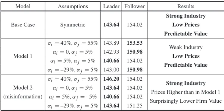
Table 1 summarizes the equilibrium forecasted by the models, given different parameters to describe the players’ expectations about the future. The prices in bold letters refer to the more viable Firm j, while in the column of Results the bold letters highlight the positive outcomes of each situation.
Table 1– Consolidated results.
Model Assumptions Leader Follower Results Strong Industry Base Case Symmetric 143.64 154.02 Low Prices
Predictable Value
Model 1
σi =40%,σj =55% 143.89 153.53
Weak Industry
αi =0,αj =5% 142.93 150.98
Low Prices
αi =5%,αj =5% 140.66 154.02
Predictable Value
αi =–29%,αj =5% 143.00 150.98
Model 2
σi =40%,σj =55% 146.20 154.02
Strong Industry
(misinformation)
αi =0,αj =5% 143.64 154.02
Prices Higher than in Model 1
αi =5%,αj =–5% 140.66 154.02
Surprisingly Lower Firm Value
αi =–29%,αj =5% 143.64 151.25
Note: the Leader and Follower columns show at what price they enter the market, in R$/MWh.
The base case scenario yields the best combination of results: energy prices for consumers are lower, the government contracts energy from firms that are economically more viable and, there-fore, with higher chances that their wind farms will be actually built. Besides that, entrepreneurs will obtain a value from its investments that tend to be in line with their original expectations, which favors new investments in the future.
When there is an asymmetry of expectations, Model 2 still favors the entry of strong players, but at the expense of higher initial and average energy prices for consumers when compared to Model 1, and entrepreneurs tend to get a value from their investments that is lower than originally expected.
5 CONCLUSIONS AND RECOMMENDATIONS
The problem was modeled as a preemption game between two characteristic firms which are asymmetric in terms of three features: the initial investment required to enter this new market (I), the net present value(V)of the standard projects that will steadily compose each firm’s portfolio and their expectations concerning the wind market prospects in the years to come. Through a sensitivity analysis, the Option-Games models identified under which conditions the less viable firm would preempt the market.
Our analysis shows that when competitors have different subjective views about the market’s perspectives, the risk of less viable firms preempting the market grows significantly when such firms believe the values of new wind projects will stay stable or decline in the future.
When market players are less informed on how competitors stand regarding their expectations about the future, there is an implicit incentive to the first entry of more viable projects, but this happens at the expense of a higher energy price for consumers.
It is noteworthy that several seminars congregating potential investors in the wind industry were held in 2009, suggesting that players may have had a reasonable grasp on the expectations of their competitors. This may have favored the entry of less viable projects first.
The model’s optimal decision is very sensitive to the stochastic process used to describe the expectation about market perspectives, specially the one used by the less viable firm. Therefore, equalizing players’ expectations as much as possible would help in the development of a strong and consistent wind industry in Brazil.
It is noticeable that in the auctions held later in 2010 and 2011, signals of the government’s strategy towards the wind industry became clearer, such as the intention to contract 1-2GW/yr, and higher capacity farms won the bids. On the other hand, energy prices dropped significantly, but according to market players this is a result of falling equipment prices due to the economic crisis that sharply reduced demand for wind generation equipment in the US and Europe.
The implication for investors is that competitors’ views about the future of the market influence their investment decisions, so efforts should be more diligently spent, in the seminars and class associations that usually precede investments in a new industry, in order to know better the com-petition. Our results show that players tend to reap a lower than expected value from their wind projects when they don’t know their opponent’s views.
The implication for government policy is that in order to avoid as much as possible contracting less viable projects with lower chances of materializing, the government should send clear and credible signals of its long term commitment to the industry, such as disclosing how much wind energy is to be contracted in the future, for example. In the 2010 and 2011 auctions, the gov-ernment contracted about 2GW/yr, and players’ expectations have aligned around this number; however, there is not, as yet, any guarantee that this governmental strategy will be maintained.
longer wind series; the site’s proximity to the grid; financial sophistication and knowledge about the industry; capacity to negotiate better state fiscal incentives, etc.). Nonetheless, our conclu-sions show that, all other variables remaining equal, the asymmetry in expectations causes sig-nificant difference in results.
As a recommendation for future research, this analysis can be expanded to include multi step games, such as the possibility that players may update their expectations about the future over time as market conditions and demand are revealed, or to model each player’s uncertainty about the stochastic process adopted by the opponent to describe the market’s risk – ambiguity – as described in the works of Nishimura & Ozaki (2007) and Roubaud, Lapied & Kast (2010).
REFERENCES
[1] ANEEL. 2011.Report on the Development of New Wind Farms. Retrieved from
http://www.aneel.gov.br/area.cfm?idArea=3.
[2] AZEVEDOA & PAXSONDA. 2010.Real Options Investment Games: A Review. Paper presented at the 14th Annual International Conference – Real Options Group. Retrieved from
https://www.realoptions.org/papers2010/109.pdf.
[3] BATISTA FRS, TEIXEIRA JP, BAIDYATKN & MELO ACG. 2011. Avaliac¸˜ao dos M´etodos de Grat, Vora & Weeks e dos M´ınimos Quadrados na Determinac¸˜ao do Valor Incremental do Mercado de Carbono nos Projetos de Gerac¸˜ao de Energia El´etrica no Brasil.Pesquisa Operacional31(1): 135–155.
[4] BASTIAN-PINTOCL, BRANDAO˜ LET & HAHNWJ. 2009. Flexibility as a source of value in the production of alternative fuels: The ethanol case.Energy Economics,31: 411–422.
[5] BLACKF & SCHOLESM. 1973. The Pricing of Options and Corporate Liabilities.The Journal of
Political Economy,81(3): 637–654.
[6] BRANDAO˜ LE, DYERJS & HAHNWJ. 2005. Using Binomial Decision Trees to Solve Real Option Valuation Problems.Decision Analysis,2(2): 69–88.
[7] BRENNANMJ & SCHWARTZES. 1985. Evaluating Natural Resource Investments.The Journal of
Business,58(2): 135–157.
[8] COPELANDT & ANTIKAROVA. 2003.Real Options: A Practitioner’s Guide. Texere, New York. [9] COSTACV, LAROVEREE & ASSMANND. 2008. Technological innovation policies to promote
renewable energies: Lessons from the European experience for the Brazilian case. [doi: DOI: 10.1016/j.rser.2006.05.006].Renewable and Sustainable Energy Reviews,12(1): 65–90.
[10] DIASACAM, BASTIAN-PINTOCL, BRANDAO˜ LET & GOMESLL. 2011. Flexibility and uncer-tainty in agribusiness projects: investing in a cogeneration plant. RAM.Revista de Administrac¸˜ao
Mackenzie,12: 105–126.
[11] DIXITAK & PINDYCKRS. 1994.Investment under Uncertainty. Princeton: Princeton University Press.
[12] EPE – EMPRESA DE PESQUISA ENERGETICA´ . 2008. PDEE – Plano Decenal de Expans ˜ao de
[13] FENOLIOLMS & MINARDIAMAF. 2009. Applying real options theory to the valuation of small hydropower plants.Revista de Economia e Administrac¸ ˜ao,8: 347–369.
[14] GIBBONSR. 1992. A Primer in Game Theory. Pearson Education Ltd: Harlow.
[15] GOMESLL & LUIZIG. 2009. Valor Adicionado aos Consumidores Livres de Energia El´etrica no Brasil por Contratos Flex´ıveis: Uma Abordagem pela Teoria das Opc¸˜oes.REAd – Revista Eletr ˆonica
de Administrac¸˜ao,15: 1–27.
[16] GRENADIERS. 2000.Game Choices: The Intersection of Real Options and Game Theory: Risk Books.
[17] GRENADIERSR. 1996. The Strategic Exercise of Options: Development Cascades and Overbuilding in Real Estate Markets.The Journal of Finance,51(5): 1653–1679.
[18] HUISMANKJM & KORT P. 2001. Technology and Symmetric Firms.Technology Investment: A
game theoretical real options approach(pp. 147–169).
[19] HUISMANKJM & NIELSENM. 2001. One Technology and Asymmetric Firms.Technology
Invest-ment: A game theorical real options approach(pp. 272): Kluwer Academic Publishers.
[20] LEAHY JV. 1993. Investment in Competitive Equilibrium: The Optimality of Myopic Behavior.
The Quarterly Journal of Economics,108(4): 1105–1133.
[21] LEMAA & RUBYK. 2007. Between fragmented authoritarianism and policy coordination: Creating a Chinese market for wind energy.Energy Policy,35(7): 3879–3890.
[22] MCDONALDR & SIEGELD. 1986. The Value of Waiting to Invest.The Quarterly Journal of
Eco-nomics,101(4): 707–728.
[23] MERTONRC. 1973. Theory of Rational Option Pricing.Bell Journal of Economics and Management
Science(4), 141–183.
[24] NISHIMURAKG & OZAKIH. 2007. Irreversible investment and Knightian uncertainty. [doi: DOI: 10.1016/j.jet.2006.10.011].Journal of Economic Theory,136(1): 668–694.
[25] NOVAESAGN & SOUZAJC. 2005. A Real Options Approach to a Classical Capacity Expansion Problem.Pesquisa Operaciona,25(2): 159–181.
[26] PAWLINAG & KORTPM. 2006. Real Options in an Asymmetric Duopoly: Who Benefits from Your Competitive Disadvantage?Journal of Economics & Management Strategy,15(1): 1–35.
[27] POMPERMEYERFM, FLORIAN M, LEAL JE & SOARESACA 2007. Spatial Price Equilibrium in the Oligopolistic Market for Oil Derivatives: an application to the Brazilian scenario.Pesquisa
Operacional,27(3): 517–534.
[28] ROCHAK, GARCIAFA, SALLESL, TEIXEIRAJP & SARDINHAJA. 2007. Real estate and real options – A case study.Emerging Markets Review,8: 67–79.
[29] ROUBAUDD, LAPIEDA & KASTR. 2010.Real Options under Ambiguity. Paper presented at the International Annual Real Options Conference 2010.
[30] SCHELLINGT. 1960.Strategy of Conflict: Harvard University Press. USA.
[31] SMETSF. 1991. Exporting versus FDI: The effect of uncertainty, irreversibilities and strategy inter-actions. Yale University.
[33] SMITHYJ & ANKUMLA. 1993. A Real Options and Game-Theoretic approach to corporate invest-ment strategy under competition.Financial Management, 241–250.
[34] TOURINHOOAF. 1979.The valuation of reserves of natural resources: an option pricing approach.
University of California, Berkeley.
[35] TRIGEORGISL. 1993. Real Options and Interactions with Financial Flexibility.Financial Manage-ment,22(3): 202–224.
[36] WWEA. 2012. World Wind Energy Half-Year Report 2012. World Wind Energy Association. Avail-able at:http://www.wwindea.org/webimages/Half-year\_report\_2012.pdf.
APPENDIX A: VALUE FUNCTIONS
The value functions are the solutions to the differential equations that describe the optimization problem faced by a firm that holds an option to enter a new market, subject to an uncertaintyY. A general partial differential equation will be detailed first, and adapted later on to the problem’s specific assumptions.
Consider a firm that holds a perpetual American option to invest in a project subject to a stochastic variableY, which follows a Geometric Brownian Motion (GBM) diffusion process. This means the firm can exercise the option to invest any time, with no time constraint, and thatY varies in time according to Eq. (A.1).
dY =αY dt+σY d z (A.1)
whereαis the drift – the expected trend ofY−,σis the standard deviation, andd z=ξ√dtis a random Wiener increment, beingdta small interval of time andξ ∼N(0,1).
The value F of this firm can be stated as a maximization problem, as in Bellman’s equation in dynamic programming (see Dixit & Pindyck, 1994, p. 95-109):
F(Y(t))=max
(Y);π(Y)+ 1
1+ρE[F(Y(t+1))|Y(t)]
(Y)is the expected value when the option is exercised, π(Y)are whatever cash flows are generated while the option is still alive (in the Follower case, it is zero),ρis the opportunity cost.
The first term of this maximization equation refers to the firm’s value if it does invest, while the second term describes the continuation value, that is, the firm’s value if it opts to continue waiting to invest. When the first term exceeds the second, the firm will stop waiting and will invest, so this is an optimal stopping problem. While waiting, the firm’s value is:
F(Y(t))=π(t)dt+ 1
1+ρdtE[F(Y(t+dt))],
which can be simplified by applying simple algebra:
F(Y(t)).(1+ρdt)=π(t)dt.(1+ρdt)+E[F(Y(t))+d F]
For a smalldt,dt2tends to zero, so: ρFdt=πdt+E[d F], in a simpler notation, or:
ρF=π+ 1
dtE[d F] (A.2)
Itˆo’s Lemma (see Eq. A.3), an equivalent in stochastic calculus to a Taylor series expansion, allows to differentiate functions of stochastic processes, such as Eq. (A.2).
d F= ∂F ∂t dt+
∂F ∂YdY+
1 2
∂2F ∂Y2(dY)
2
or, in a simpler notation:
d F=Ftdt+FYdY+ 1
2FY Y(dY)
2 (A.3)
From Eq. (A.1),dY2=α2Y2dt2+2αY2σdt d z+σ2Y2d z2. The first and second terms to the right, which are indt3/2anddt2, vanish in the limit. As a result:
dY2=σ2Y2d z2 (A.4)
Before proceeding, recall that:d z2=ξ2dt; beingξ∼N(0,1),E[ξ] =0, and:VAR(ξ )=1=> E[ξ2] −E2[ξ] =1=>E[ξ2] =1+0=1; as a result: E[d z2] = E[ξ2dt] =dt.E[ξ2] =dt, andVAR(d z2)=VAR(ξ2dt)=dt2.VAR(ξ2)∼zero. As a result,d z2=dt, and Eq. (A.4) can be rewritten as:
d F=Ftdt+FY(αY dt+σY d z)+ 1 2FY Y(σ
2Y2dt)
E[d F] =E[Ftdt+FY(αY dt+σY d z)+ 1 2FY Y(σ
2Y2dt) ]
E[d F] =Ftdt+αY FYdt+σY FY √
dt.E[ξ] +1 2FY Y(σ
2Y2dt)
; as E[ξ] =0,
E[d F] =Ftdt+αY FYdt+ 1 2σ
2Y2F
Y Ydt (A.5)
Combining Eq. (A.5) and Eq. (A.2):
ρF =π+ 1 dt
Ftdt+αY FYdt+ 1 2σ
2Y2F Y Ydt
, or:
1 2σ
2Y2F
Y Y +αY FY +Ft−ρF+π =0 (A.6)
In addition, the new market assumption translates into firmsiandj having no cash flows before investing. When in the position of Follower,π is zero and the ordinary differential equation is reduced to its homogeneous part: 12σ2Y2FY Y +αY FY−ρF =0 or, in simpler notation:
1 2σ
2Y2F′′
+αY F′−ρF =0 (A.7)
One tentative solution to Eq. (A.7) is:
F =A.Yβ (A.8)
Finding the second and first derivatives of F in respect to the state variableY and substituting the results in Eq. (A.7), it can be rewritten only on the parameters ofY’s stochastic process,α andσ:
1 2σ
2β(β
−1)+αβ−ρ=0 (A.9)
Eq. (A.9) is quadratic and its roots are:
β1 = 1
2σ2−α+
α−12σ2
2
+2σ2ρ
σ2 and
β2 = 1
2σ2−α−
α−12σ2 2+2σ2ρ
σ2
So, the general solution to the homogeneous part of the differential equation is: F = A1Yβ1 +
A2Yβ2, beingβ
1>1 andβ2<0.
A2can be found using common sense: whenY tends to zero, F should also tend to zero, and this is only feasible ifA2is zero (a negativeβ2makes that term inA2tend to∞whenY tends to zero). So the solution to the differential equation of the firm with the option to invest as Follower is simply:
F= A1Yβ1 (A.10)
For the firm that is already the Leader, the differential equation also includes a non homoge-neous term,π, which reflects the cash flows reaped before the Follower enters the market (see Eq. (A.6)). In this case, the solution includes not only the solution to the homogeneous part of the differential equation, but also a specific solution. A natural tentative for this specific solution is to use the firm’s value if the competitor never entries the market, a perpetuity: ρπ−α. However, any other specific solution that is adequate to describe the problem and also satisfies Eq. (A.6) is acceptable. In case of a perpetuity, the solution to the differential equation of the firm with the option to invest as Leader is in Eq. (A.11):
F= AYβ1+ π
Equations (A.10) and (A.11) are the basic frameworks of the value functions of the Follower and the Leader, respectively, while their options to invest are still alive. In order to find which value of Y triggers investment, the expected values of the firms upon exercising their options (equivalent to the(Y)term in Bellman’s equation) must be estimated, and the boundary conditions that separate the two possible states (didn’t invest/invested) must also be defined. They are detailed below. From this point on, subscriptsi or j are included in the equations, just to clarify which firm is being addressed, followed by another subscript,L or F, indicating if the firm is in the condition of Leader or Follower.
MODEL 1 – BOTH FIRMS GUESS CORRECTLY WHAT THE OPPONENT THINKS ABOUT THE FUTURE
Situation 1: Firmiis the Leader, Firm jis the Follower
Assuming Firmihas already invested, Firm j will only invest whenYj is sufficiently high, that is, when it has exceeded a certain valueY∗j Fwhich triggers Firmjto invest as Follower, and that happens at timet =τ∗j F =inf(t|Y(t)≥Y∗j F).
Follower (Firm j)
Eq. (A.12) is similar to Eq. (A.10) and it reflects the firm’s value when the option to enter the market is still alive, while Equation (A.13) describes its value upon entering the market as a Follower.
Fj(Yj)=AY βj
j , in the continuation region, that is, whenYj ≤Y∗j F (A.12)
Fj(Yj)=
YjDj11(1+αj)
ρ−αj +
YjDj11−Ij =
YjDj11(1+ρ)
ρ−αj −
Ij, whenYj ≥Y∗j F (A.13)
In Equation (A.13), the first term to the right reflects the firm’s expected value considering that it will add, in perpetuity, new standard wind farms to its portfolio; the second term reflects the net present value of the first standard wind farm built (that is, the firstV); the third term,I j, reflects the costs to establish a foothold in this market.
The assumption of a new standard project being added in perpetuity is not mandatory; it is adopted here, at this point of our text, just for the purpose of presenting the value equations in a format that is more easily comparable to those used in other Option-Games papers. The assumption may, instead, be that each firm will add new standard wind farms to the portfolio for the nextxyears; in this case, when Firm jenters the market it will reap the following expected value:
Fj(Yj)=YjDj11−Ij+YjDj11
(1+αj)
1+ρ) +YjDj11
(1+αj)2
(1+ρ)2 + · · · +YjDj11
(1+αj)2 (1+ρ)2
Therefore, Eq. (A.13) can also be stated as:
being
κj =
1+(1+αj) (1+ρ) +
(1+αj)2 (1+ρ)2 +
(1+αj)3
(1+ρ)3 + · · · +
(1+αj)x (1+ρ)x
, (A.15)
in the cases when a limited number of farms will compose the firm’s portfolio, to be steadily built inxyears. In summary, Firmj’s value equations as Follower are:
Fj(Yj) = AY βj
j , in the continuation region, forYj ≤Y∗j F (A.12)
Fj(Yj) = κjYjDj11−Ij, forYj ≥Y∗j F (A.14)
At theYj F∗ frontier, boundary conditions are necessary to guarantee the continuity between func-tions (A.12) and (A.14) –Value Matching Condition, VMC – and theSmooth Pasting Condition, SPC, which means that the derivatives or the slopes of Eqs. (A.12) and (A.14) match when they touch atYj F∗ . Please refer to Dixit & Pindyck (1994, p. 130-132) for a brief explanation on these boundary conditions. Therefore:
VMC:AYj F∗βj =κjY∗j FDj11−Ij
SPC:βjAY∗ βj−1
j F =κjDj11, so
A = κjDj11
Y∗j F1−βj
βj
and (A.16)
Y∗j F = βj (βj−1)
Ij
κjDj11
, where (A.17)
βj = 1
2σ2j −αj+
αj−12σ2j2+2ρσ2j
σ2j (A.18)
Equations (A.12), (A.14), (A.15), (A.16), (A.17), (A.18) define the value curves of Firm j as Follower.
Leader (Firmi)
The differential equation that describes the Leader is: 12σiYi2F ′′
i +αiYiFi′ −ρF +πi = 0. Following similar procedures, the value curves of Firmias Leader are:
Fi(Yi)=BYiθi +(κiYiDi10−Ii),in the continuation region, that is, forYj ≤Y∗j F (A.19)
Fi(Yi)=κiYiDi11−Ii, forYj ≥Y∗j F (A.20)
κi =
1+(1+αi) (1−ρ) +
(1+αi)2 (1+ρ)2 +
(1+αi)3
(1+ρ)3 + · · · +
(1+αi)x (1+ρ)x
It is noteworthy that the Leader holds no option, here (it has already exercised its option to enter the market); the Leader’s value function actually reflects what happens to the Leader’s value in light of the chances that the Follower will exercise its option to also enter the market. So, the term in brackets in the right-hand side of Equation (A.19) reflects the Leader’s value if the opponent never enters the market, while the first term reflects the erosion in the Leader’s value, given the risk that the opponent will also enter the market. So, constantBmust be negative, reflecting that whenY grows, the risk that the competitor will enter the market also grows – and higher is the erosion in the Leader’s value.
Y∗j F has already been found – Equation (A.17) –, while constantBcan be obtained by using the value matching condition (VMC), that is, by equaling Equations (A.19) and (A.20), at the point whenYi =Yj =Y∗j F. As a result:
B = κi(Di11−Di10)Yj F∗1−θi (A.22)
θi = 1
2σi2−αi+
αi−12σi22+2ρσi2
σi2 (A.23)
Rootθi reflects Firmi’s own expectations about the wind market’s future: it expects the oppo-nent will enter the market whenY reachesY∗j F, but the speed/probability at whichY will reach this trigger is commanded by the stochastic process adopted by Firmi to describe the market’s perspectives. In summary, Equations (A.19), (A.20), (A.21), (A.22) and (A.23) define the value curves of the Leader.
Firmi starts to get encouraged to become the Leader as soon as its value as Leader exceeds its value as Follower (the latter, obtained following the same steps previously used to develop the value functions for Firm j, when as Follower). This incentive happens atY =Yi P, at time
t = inf(t|FiLeader ≥ FiFollower). However, Firmi not necessarily preempts the market at this moment; if there is no risk the opponent will preempt the market first, Firmi may wait for a more favorable realization ofY, that is, Firm i’s option to wait is still valuable. As a result, Firmi may wait until timet = inf(t|FjLeader ≥ FjFollower), a little before its opponent is also encouraged to enter as Leader, and this happens atY =Yj P. In summary, Firmi preempts the market atYj P−ǫ.
There is another subtlety, though: is it still worthy waiting? When Firmi keeps its option to invest as Leader alive, its value is described by:
Fi(Yi)=MYiθi (A.24)
It is only worthy waiting if the value while waiting exceeds the value already as the Leader, which is described by Equations (A.19) and (A.20). The optimal stopping moment can again be devised by applying the value matching and smooth pasting conditions (VMC, SPC) to Equations (A.19) and (A.24). We define that this optimal stopping point is atY =Yi∗. So:
VMC:MY∗θi
i =BY∗ θi
SPC:θiMYi∗θi−1=θiBYi∗θi−1+κiDi10
As a result:
Yi∗ = θi θi−1 ·
Ii κiDi10
(A.25)
M = B+Y
∗(1−θi)
i θi
κiDi10 (A.26)
Depending on the parameters of the problem,Yi∗may be higher of lower thanYj P. Therefore, Firmiwill actually enter the market as Leader when (please recall Fig. 3):
a) Yi L∗ =Yi∗, ifYi∗ <Yj P; in this case, Firmidecides to enter the market at the same point it would enter if it were a monopolist (Leahy, 1993).
b) Yi L∗ =Yj P−ǫ, ifYi∗≥Yj P; Firmienters the market a little before the opponent is also encouraged to enter as Leader.
Situation 2: Firm jis the Leader, Firmiis the Follower
Following procedures similar to those used in Situation 1, we obtain the value functions of the Leader and the Follower.
Follower (Firmi)
Fi(Yi) = CYiθi, in the continuation region, forYi ≤Yi F∗ (A.27)
Fi(Yi) = κiYiDi11−Ii, forYi ≥Yi F∗ (A.28)
C = κiDi11
Y∗1−θi i F
θi
(A.29)
Yi F∗ = θi (θi −1)
Ii κiDi11
(A.30)
Leader (Firm j)
Fj(Yj) = EY βj
j +(κjYjDj01−Ij), in the continuation region, whereYi ≤Yi F∗ (A.31)
Fj(Yj) = κjYjDj11−Ij, forYi ≥Yi F∗ (A.32)
E = κj(Dj11−Dj01)Y∗1− βj
i F (A.33)
The Leader’s trigger when in monopoly is:
Y∗j = βj βj−1
Ij κjDj01
Firm j’s value when the option to enter the market as Leader is still alive is:
Fj(Yj)=N Y βj
j (A.35)
N =E+Y
∗(1−βj)
j
βj
κjDj01 (A.36)
MODEL 2 – THE IMPACT OF MISINFORMATION
Each player, not knowing what the opponent thinks about the future, wrongly assumes that they both share the same expectation about the market, basing their decisions on the same stochastic process. From the point of view of each player, the problem is solved as a duopoly with only two asymmetries, those related to their economic viability – the net present value of each firm’s standard project,V, and the investment I to establish a foothold in the wind market. However, each player will only use its own stochastic process to describe the market’s perspectives. Each firm expects the opponent to enter the market when triggered by certain market conditions, but will be surprised by the opponent, which will make decisions based on their own stochastic process. This alters the expected value of the Leader. The triggers for the Leader and the Follower can be derived as in Model 1.
Situation 1: Firmias Leader, Firm jas Follower
Firmiassumes the competitor, Firmj, will enter as Follower at:
Yj F∗ = θi (θi−1)
Ij
κiDj11
(A.37)
Equations (A.19), (A.20), (A.21), (A.22), (A.23), (A.37) describe the Leader’s value curves. However, Firm j tends to enter as a Follower at the moment described by Equation (A.17), not at the moment described by Equation (A.37).
Situation 2: Firm j as Leader, Firmias Follower
Likewise, the Leader’s decision is based on the assumption that the Follower will enter the market at:
Yi F∗ = βj (βj −1)
Ii κjDi11
(A.38)