fields
Tony Lindeberg*
Department of Computational Biology, School of Computer Science and Communication, KTH Royal Institute of Technology, Stockholm, Sweden
Abstract
The brain is able to maintain a stable perception although the visual stimuli vary substantially on the retina due to geometric transformations and lighting variations in the environment. This paper presents a theory for achieving basic invariance properties already at the level of receptive fields. Specifically, the presented framework comprises (i) localscaling transformationscaused by objects of different size and at different distances to the observer, (ii) locallylinearized image deformationscaused by variations in the viewing direction in relation to the object, (iii) locallylinearized relative motions between the object and the observer and (iv) localmultiplicative intensity transformationscaused by illumination variations. The receptive field model can be derivedby necessityfrom symmetry properties of the environment and leads to predictions about receptive field profiles in good agreement with receptive field profiles measured by cell recordings in mammalian vision. Indeed, the receptive field profiles in the retina, LGN and V1 are close to ideal to what is motivated by the idealized requirements. By complementing receptive field measurements with selection mechanisms over the parameters in the receptive field families, it is shown how true invariance of receptive field responses can be obtained under scaling transformations, affine transformations and Galilean transformations. Thereby, the framework provides a mathematically well-founded and biologically plausible model for how basic invariance properties can be achieved already at the level of receptive fields and support invariant recognition of objects and events under variations in viewpoint, retinal size, object motion and illumination. The theory canexplainthe different shapes of receptive field profiles found in biological vision, which are tuned to different sizes and orientations in the image domain as well as to different image velocities in space-time, from a requirement that the visual system should be invariant to the natural types of image transformations that occur in its environment.
Citation:Lindeberg T (2013) Invariance of visual operations at the level of receptive fields. PLoS ONE 8(7): e66990. doi:10.1371/journal.pone.0066990 Editor:Luis M Martinez, CSIC-Univ Miguel Hernandez, Spain
ReceivedOctober 16, 2012;AcceptedMay 14, 2013;PublishedJuly 19, 2013
Copyright:ß2013 Tony Lindeberg. This is an open-access article distributed under the terms of the Creative Commons Attribution License, which permits unrestricted use, distribution, and reproduction in any medium, provided the original author and source are credited.
Funding:Funding was received from The Swedish Research Council contract 2010–4766; The Royal Swedish Academy of Sciences; and The Knut and Alice Wallenberg foundation. The funders had no role in study design, data collection and analysis, decision to publish, or preparation of the manuscript. Competing Interests:The author has declared that no competing interests exist.
* E-mail: [email protected]
Introduction
We maintain a stable perception of our environment although the brightness patterns reaching our eyes undergo substantial changes. This shows that our visual system possesses invariance properties with respect to several types of image transformations: If you approach an object, it will change its size on the retina. Nevertheless, the perception remains the same, which reflects a
scale invariance. It is well-known that humans and other animals have functionally important invariance properties with respect to variations in scale. For example, Biederman and Cooper [1] demonstrated that reaction times for recognition of line drawings were independent of whether the primed object was presented at the same or a different size as when originally viewed. Logothetiset al.[2] found that there are cells in the inferior temporal cortex (IT) of monkeys for which the magnitude of the cell’s response is the same whether the stimulus subtended10or60of visual angle. Itoet al.[3] found that about 20 percent of anterior IT cells responded to ranges of size variations greater than 4 octaves, whereas about 40 percent responded to size ranges less than 2 octaves. Furmanski and Engel [4] found that learning with application to object recognition transfers across changes in image size. The neural mechanisms underlying object recognition are rapid and lead to
scale-invariant properties as soon as 100–300 ms after stimulus onset (Hunget al.[5]).
In a similar manner, if you rotate an object in front of you, the projected brightness pattern will be deformed on the retina, typically by different amounts in different directions. To first order of approximation, such image deformations can be modelled by local affine transformations, which include the effects of in-plane
rotationsand perspectiveforeshortening. For example, Logothetiset al.
[2] and Booth and Rolls [6] have shown that in the monkey IT cortex there are both neurons that respond selectively to particular views of familiar objects as well as populations of single neurons that have view-invariant representations over different views of familiar objects. Edelmann and Bu¨lthoff [7] have on the other hand shown that the time for recognizing unfamiliar objects from novel views increases with the 3-D rotation angle between the presented and previously seen views. Still, subjects are able to recognize unfamiliar objects from novel views, provided that the 3-D rotation is moderate.
If an object moves in front of you, it may in addition to a
approximation be modelled by local Galilean transformations. Regarding biological counterparts of such relative motions, Rodman and Albright [8] and Lagaeet al.[9] have shown that in area MT of monkeys there are neurons with high selectivity to the speed and direction of visual motion over large ranges of image velocities. Petersenet al.[10] have shown that there are neurons in area MT that adapt their response properties to the direction and velocity of motion. Smeets and Brenner [11] have shown that reaction times for motion perception can be different for absolute and relative motion and that reaction times may specifically depend on the relative motion between the object and the background. When Einstein derived his relativity theory, he used as a basic assumption the requirement that the equations should be invariant under Galilean transformations [12].
The measured luminosity of surface patterns in the world may in turn vary over several orders of magnitude. Nevertheless we are able to preserve the identity of an object as we move it out of or into a shade, which reflects important invariance properties under
intensity transformations. The Weber-Fechner law states that the ratio of an increment threshold DI in image luminosity for a just noticeable difference in relation to the background intensityI is constant over large ranges of luminosity variations (Palmer [13, pages 671–672]). The pupil of the eye and the sensitivity of the photoreceptors are continuously adapting to ambient illumination (Hurley [14]).
To be able to function robustly in a complex natural world, the visual system must be able to deal with these image transforma-tions in an efficient and appropriate manner to maintain a stable perception as the brightness pattern changes on the retina. One specific approach is by computinginvariant featureswhose values or representations remain unchanged or only moderately affected under basic image transformations. A weaker but nevertheless highly useful approach is by computing visual representations that possess suitable covariance properties, which means that the repre-sentations are transformed in a well-behaved and well-understood manner under corresponding image transformations. A covariant image representation can then in turn constitute the basis for computing truly invariant image representations, and thus enable invariant visual recognition processes at the systems level, in analogy with corresponding invariance principles as postulated for biological vision systems by different authors (Rolls [15]; DiCarlo and Maunsell [16]; Grimes and Rao [17]; [18]; DiCarlo and Cox [19]; Goris and Beek [20]).
The subject of this paper is to introduce a computational framework for modelling receptive fields at the earliest stages in the visual system corresponding to the retina, LGN and V1 and to show how this framework allows for basic invariance or covariance properties of visual operationswith respect to all the above mentioned phenomena. This framework can be derived fromsymmetry properties
of the natural environment (Lindeberg [21,22]) and leads to predictions ofreceptive field profilesin good agreement with receptive measurements reported in the literature (Hubel and Wiesel [23– 25]; DeAngeliset al.[26,27]). Specifically, explicit phenomenolog-ical models will be given of LGN neurons and simple cells in V1 and be compared to related models in terms of Gabor functions (Marcˇelja [28]; Jones and Palmer [29,30]), differences of Gaussians (Rodieck [31]) or Gaussian derivatives (Koenderink and van Doorn [32]; Young [33]; Young et al. [34,35]). Notably, the evolution properties of the receptive field profiles in this model can be described by diffusion equations and are therefore suitable for implementation on a biological architecture, since the computa-tions can be expressed in terms of communicacomputa-tions between neighbouring computational units, where either a single compu-tational unit or a group of compucompu-tational units may be interpreted
as corresponding to a neuron or a group of neurons. Specifically, computational models involving diffusion equations arise in mean field theory for approximating the computations that are performed by populations of neurons (Omurtaget al.[36]; Mattia and Guidic [37]; Faugeraset al.[38]).
The symmetry properties underlying the formulation of this theory will be described in the section ‘‘Model for early visual pathway in an idealized vision system’’ and reflect the desirable properties of an idealized vision system that (i) objects at different positions, scales and orientations in image space should be processed in a structurally similar manner, and (ii) objects should be perceived in a similar way under variations in viewing distance, viewing direction, relative motion in relation to the observer and illumination variations.
Combined with complementaryselection mechanisms over recep-tive fields at different scales (Lindeberg [39]), receprecep-tive fields adapted to different affine image deformations (Lindeberg and Ga˚rding [40]) and different Galilean motions (Lindeberg et al.
[21,41]), it will also be shown how true invariance of receptive field responses can be obtained with respect to local scaling transfor-mations, affine transformations and Galilean transformations. These selection mechanisms are based on either (i) the computa-tion of local extrema over the parameters of the receptive fields or alternatively based on (ii) comparisons of local receptive field responses to affine invariant or Galilean fixed-point requirements (to be described later). On a neural architecture, these geometric invariance properties are therefore compatible with a routing mechanism (Olshausenet al.[42]) that operates on the output from families of receptive fields that are tuned to different scales, spatial orientations and image velocities. In this respect, the resulting approach will bear similarity to the approach by Riesenhuber and Poggio [43], where receptive field responses at different scales are routed forward by a soft winner-take-all mechanism, with the theoretical additions that the invariance properties over scale can here be formally proven and the presented framework specifically states how the receptive fields should be normalized over scale. Furthermore, our approach extends to true and provable invariance properties under more general affine and Galilean transformations.
A direct consequence of these invariance properties established for receptive field responses is that they can be propagated to invariance properties of visual operations at higher levels, and thus enable invariant recognition of visual objects and events under variations in viewing direction, retinal size, object motion and illumination. In this way, the presented framework provides a computational theory for how basic invariance properties of a visual system can achieved already at the level of receptive fields. Another consequence is that the presented framework could be used for
explainingthe families of receptive field profiles tuned to different orientations and image velocities in space and space-time that have been observed in biological vision from a requirement of that the corresponding receptive field responses should be invariant or covariant under corresponding image transformations. A main purpose of this article is to provide asynthesiswhere such structural components are combined into a coherent framework for achieving basic invariance properties of a visual system and relating these results, which have been derived mathematically, to corresponding functional properties of neurons in a biological vision system.
for explicit incorporation of basic image transformations into computational neuroscience models of vision. If such image transformations are not appropriately modelled and if the model is then exposed to test data that contain image variations outside the domain of variabilities that are spanned by the training data, then an artificial neuron model may have severe problems with robustness. If on the other hand the covariance properties corresponding to the natural variabilities in the world underlying the formation of natural image statistics are explicitly modelled and if corresponding invariance properties are built into the computational neuroscience model and also used in the learning stage, we argue that it should be possible to increase the robustness of a neuro-inspired artificial vision system to natural image variations. Specifically, we will present explicit computational mechanism for obtaining true scale invariance, affine invariance, Galilean invariance and illumination invariance for image measurements in terms of local receptive field responses.
Interestingly, the proposed framework for receptive fields can be derived by necessity from a mathematical analysis based on symmetry requirements with respect to the above mentioned image transformations in combination with a few additional requirements concerning the internal structure and computations in the first stages of a vision system that will be described in more detail below. In these respects, the framework can be regarded as both (i) a canonical mathematical model for the first stages of processing in an idealized vision system and as (ii) a plausible computational model for biological vision. Specifically, compared to previous approaches of learning receptive field properties and visual models from the statistics of natural image data (Field [44]; van der Schaaf and van Hateren [45]: Olshausen and Field [46]; Rao and Ballard [47]; Simoncelli and Olshausen [48]; Geisler [49]) the proposed theoretical model makes it possible to determine spatial and spatio-temporal receptive fields from first principles that reflect symmetry properties of the environment and thus without need for any explicit training stage or gathering of representative image data. In relation to such learning based models, the proposed normative approach can be seen as describing the solutions that an ideal learning based system may converge to, if exposed to a sufficiently large and representative set of natural image data. The framework for achieving true invariance properties of receptive field responses is also theoret-ically strong in the sense that the invariance properties can be formally proven given the idealized model of receptive fields.
In their survey of our knowledge of the early visual system, Carandiniet al.[50] emphasize the need for functional models to establish a link between neural biology and perception. More recently, Einha¨user and Ko¨nig [51] argue for the need for normative approaches in vision. This paper can be seen as developing the consequences of such ways of reasoning by showing how basic invariance properties of visual processes at the systems level can be obtained already at the level of receptive fields, using a normative approach.
Model for early visual pathway in an idealized vision system
In the following we will state a number of basic requirements concerning the earliest levels of processing in an idealized vision system, which will be used for derivingidealized functional models of receptive fields. Let us stress that the aim is not to model specific properties of human vision or any other species. Instead the goal is to describe basic characteristics of the image formation process and the computations that are performed after the registration of image luminosity on the retina. These assumptions will then be
used for narrowing down the class of possible image operations that are compatible with structural requirements, which reflect symmetry properties of the environment. Thereafter, it will be shown how this approach applies to modelling of biological receptive fields and how the resulting receptive fields can be regarded as biologically plausible.
For simplicity, we will assume that the image measurements are performed on a planar retina under perspective projection. With appropriate modifications, a corresponding treatment can be performed with a spherical camera geometry.
Let us therefore assume that the vision system receives image data that are either defined on a (i)purely spatial domainf(x)or a (ii)
spatio-temporal domainf(x,t) withx~(x1,x2)T. Let us regard the purpose of the earliest levels of visual representations as computing a family of internal representationsL from f, whose output can be used as input to different types of visual modules. In biological terms, this would correspond to a similar type of sharing as V1 produces output for several downstream areas such as V2, V4 and V5/MT.
An important requirement on these early levels of processing is that we would like them to beuncommittedoperations without being too specifically adapted to a particular task that would limit the applicability for other visual tasks. We would also desire auniform structureon the first stages of visual computations.
Spatial (time-independent) image data
Concerning terminology, we will use the convention that a receptive field refers to a regionVin visual space over which some computations are being performed. These computations will be represented by an operator T, whose support region is V. Generally, the notion of a receptive field will be used to refer to both the operatorTand its support regionV. In some cases when referring specifically to the support regionVonly, we will refer to it as the support region of the receptive field.
Given a purely spatial image f :R2?R, let us consider the problem of defining a family of internal representations
L(:; s)~Tsf ð1Þ
for some family of operators Ts that are indexed by some parameters, where s~(s1, ,sN) may be a multi-dimensional parameter withNdimensions. (The dot ‘‘:’’ at the position of the first argumentxofLmeans thatL(:;s)when given a fixed value of the parametersonly should be regarded as a function overx.) In the following we shall state a number of structural requirements on a visual front-end as motivated by the types of computations that are to be performed at the earliest levels of processing in combination with symmetry properties of the surrounding world. Linearity. Initially, it is natural to requireTs to be a linear operator, such that
Ts(a1f1za2f2)~a1Tsf1za2Tsf2 ð2Þ
holds for all functions f1,f2:R2?R and all scalar constants
a1,a2[R. An underlying motivation to this linearity requirement is that the earliest levels of visual processing should make as few irreversible decisions as possible.
manner irrespective of what types of linear filters they are captured by.
Translational invariance. Let us also require Ts to be a
shift-invariant operatorin the sense that it commutes with the shift operatorSDx defined by(SDxf)(x)~f(x{Dx), such that
TsðSDxfÞ~SDxðTsfÞ ð3Þ
holds for all Dx. The motivation behind this assumption is the basic requirement that the perception of a visual object should be the same irrespective of its position in the image plane. Alternatively stated, the operatorTscan be said to behomogeneous
across space.
For us humans and other higher mammals, the retina is obviously not translationally invariant. Instead, finer scale receptive fields are concentrated to the fovea in such a way that the minimum receptive field size increases essentially linearily with eccentricity. With respect to such a sensor space, the assumption about translational invariance should be taken as an idealized model for the region in space where there are receptive fields above a certain size.
Convolution structure. Together, the assumptions of line-arity and shift-invariance imply that the internal representations L(:; s)are given byconvolution transformations
L(x; s)~(T(:;s)f)(x)~ ð
j[R2
T(j;s)f(x{j)dj ð4Þ
whereT(:; s)denotes some family of convolution kernels. Later, we will refer to these convolution kernels as receptive fields.
The issue of scale. A fundamental property of the convo-lution operation is that it may reflect different types of image structures depending on the spatial extent (the width) of the convolution kernel.
N
Convolution with alarge supportkernel will have the ability to respond to phenomena atcoarse scales.N
A kernel withsmall supportmay on the other hand only capture phenomena atfine scales.From this viewpoint it is natural to associate an interpretation of
scalewith the parametersand we will assume that the limit case of the internal representations whenstend to zero should correspond to the original image patternf
lim s;0L(
:;s)~lim s;0Tsf
~f: ð5Þ
Semi-group structure. From the interpretation of s as a scale parameter, it is natural to require the image operatorsTsto form asemi-groupovers
Ts1Ts1~Ts1zs2 ð6Þ
with a corresponding semi-group structure for the convolution kernels
T(:; s1)T(:;s2)~T(:; s1zs2) ð7Þ
such that the composition of two different receptive fields coupled in cascade will also be a member of the same receptive field family.
Then, the transformation between any different and ordered scale levelsssands2withs2§s1will obey thecascade property
L(:; s2)~T(:;s2{s1)T(:;s1)f
~T(:; s2{s1)L(:;s1) ð8Þ
i.e.a similar type of transformation as from the original dataf. An image representation with these properties is referred to as a multi-scale representation.
Concerning the parameterization of this semi-group, we will in the specific case of a one-dimensional (scalar) scale parameter assume the parameters[Rto have a direct interpretation of scale, whereas in the case of a multi-dimensional parameter s~(s1,. . .,sN)[RN, these parameters could also encode for other properties of the convolution kernels in terms of the orientationh
in image space or the degree of elongatione~s1=s2, wheres1 and s2 denote the spatial extents in different directions. The convolution kernels will, however, not be be required to form a semi-group over any type of parameterization, such as the parametershore. Instead, we will assume that there exists some parameterization s for which an additive linear semi-group structure can be defined and from which the latter types of parameters can then be derived.
Self-similarity over scale. Regarding the family of convo-lution kernels used for computing a multi-scale representation, it is also natural to require them toself-similar over scale, such that ifsis a one-dimensional scale parameter then all the kernels correspond to rescaled copies
T(x; s)~ 1
Q(s)TT x Q(s)
ð9Þ
of some prototype kernelTTfor some transformationQ(s)of the scale parameter. Ifs[RNz is a multi-dimensional scale parameter,
the requirement of self-similarity over scale can be generalized into
T(x;s)~ 1
jdetQ(s)jTT Q(s) {1x
ð10Þ
whereQ(s) now denotes a non-singular2|2-dimensional matrix regarding a 2-D image domain andQ(s){1
its inverse. With this definition, a multi-scale representation with a scalar scale parameter s[Rz will be based on uniform rescalings of the
by the matrix square root function Q(s)~S1=2, where Sdenotes the covariance matrix that describes the spatial extent and the orientation of the affine Gaussian kernels.
Infinitesimal generator. For theoretical analysis it is pref-erable if the scale parameter can be treated as a continuous scale parameter and if image representations between adjacent levels of scale can be related by partial differential equations. Such relations can be expressed if the semi-group possesses aninfinitesimal generator
(Hille and Phillips [52])
BL~lim h;0
T(:; h)f{f
h ð11Þ
and implies that image representations between adjacent levels of scale can be related bydifferential evolution equations; for a scalar scale parameter of the form
LsL(x; s)~(BL)(x;s) ð12Þ
for some operatorBand for anN-dimensional scale parameter of the form
(DuL)(x;s)~(B(u)L)(x; s)~
~ðu1B1z. . .zuNBNÞL(x; s) ð13Þ
for any positive directionu~(u1,. . .,uN) in the parameter space withui§0for everyi. In (Lindeberg [21]) it is shown how such differential relationships can be ensured given a proper selection of functional spaces and sufficient regularity requirements over space x and scale s in terms of Sobolev norms. We shall therefore henceforth regard the internal representationsL(:; s)as differen-tiable with respect to both the image space and scale parameter(s). Non-enhancement of local extrema. For the internal representationsL(:;s)that are computed from the original image dataf it is in addition essential that the operatorsTsdo not generate
new structures in the representations at coarser scales that do not correspond to simplifications of corresponding image structures in the original image data.
A particularly useful way of formalizing this requirement is that
local extrema must not be enhanced with increasing scale. In other worlds, if a point (x0; s0) is a local (spatial) maximum of the mapping
x.L(x;s0)then the value must not increase with scale. Similarly, if a point (x0; s0) is a local (spatial) minimum of the mapping
x.L(x;s0), then the value must not decrease with scale. Given the above mentioned differentiability property with respect to scale, we say that the multi-scale representation constitutes a scale-space representation if it for a scalar scale parameter satisfies the following conditions at any non-degenerate local extremum point:
LsL(x0; s0)ƒ0 at any local maximum , ð14Þ
LsL(x0; s0)§0 at any local minimum , ð15Þ
or for a multi-parameter scale-space
(DuL)(x0; s0)ƒ0 at any local maximum , ð16Þ
(DuL)(x0;s0)§0 at any local minimum , ð17Þ
for any positive directionu~(u1,. . .,uN)in the parameter space withui§0for everyi(see figure 1).
Rotational invariance. If we restrict ourselves to a scale-space representation based on a scalar (one-dimensional) scale parameter s[Rz, then it is natural to require the scale-space
kernels to berotationally symmetric
T(x; s)~h(
ffiffiffiffiffiffiffiffiffiffiffiffiffiffi x2
1zx22 q
;s) ð18Þ
for some one-dimensional function h(:;s):R?R. Such a symmetry requirement can be motivated by the requirement that in the absence of further information, all spatial directions should be equally treated (isotropy).
For a scale-space representation based on a multi-dimensional scale parameter, one may also consider a weaker requirement of rotational invariance at the level of a family of kernels, for example regarding a set of elongated kernels with different orientations in image space. Then, the family of kernels may capture image data of different orientation in a rotationally invariant manner, for example if all image orientations are explicitly represented or if the receptive fields corresponding to different orientations in image space can be related by linear combinations.
Affine covariance. The perspective mapping from surfaces of objects in the 3-D world to the 2-D image space gives rises to image deformations in the image domain. If we approximate the non-linear perspective mapping from a surface pattern in the world to the image plane by a local linear transformation (the derivative), then we can model this deformation by an affine transformation
f0~A f ð19Þ
corresponding to
f0(x0)~f(x) with x0~A xzb ð20Þ
whereArepresents an affine transformation operator operating on functions andAis the affine transformation matrix. To ensure that the internal representations behave nicely under image deforma-tions, it is natural to require a possibility of relating them under affine transformations
L0(x0;s0)~L(x;s) ð21Þ
corresponding to
TA(s)A f~A Tsf ð22Þ
achieved with a scalar scale parameter and linear operations. As will be shown below, it can, however, be achieved with a 3-parameter linear scale-space.
Necessity result concerning spatial receptive fields Given the above mentioned requirements it can be shown that if we assume (i) linearity, (ii) shift-invariance over space, (iii) semi-group property over scale, (iv) sufficient regularity properties over space and scale and (v) non-enhancement of local extrema, then the scale-space representation over a 2-D spatial domain must satisfy (Lindeberg [21, theorem 5, page 42])
LsL~1 2+
T
xðS0+xLÞ{dT0+xL ð23Þ
for some2|2covariance matrixS0and some 2-D vectord0with
+x~(Lx
1,Lx2) T
. If we in addition require the convolution kernels to bemirror symmetricthrough the originT({x;s)~T(x;s) then the offset vector d0 must be zero. There are two special cases within this class of operations that are particularly worth emphasizing.
Gaussian receptive fields. If we require the corresponding convolution kernels to be rotationally symmetric, then it follows that they will be Gaussians
T(x;s)~g(x; s)~ 1 2pse
{xT x=2s~ 1 2pse
{(x2
1zx22)=2s ð24Þ
with corresponding Gaussian derivative operators
(Lxag)(x;s)~(L
xa11xa22g)(x1,x2; s)
~(L
x1a1gg)(x1; s) (Lx2a2gg)(x2; s) ð25Þ
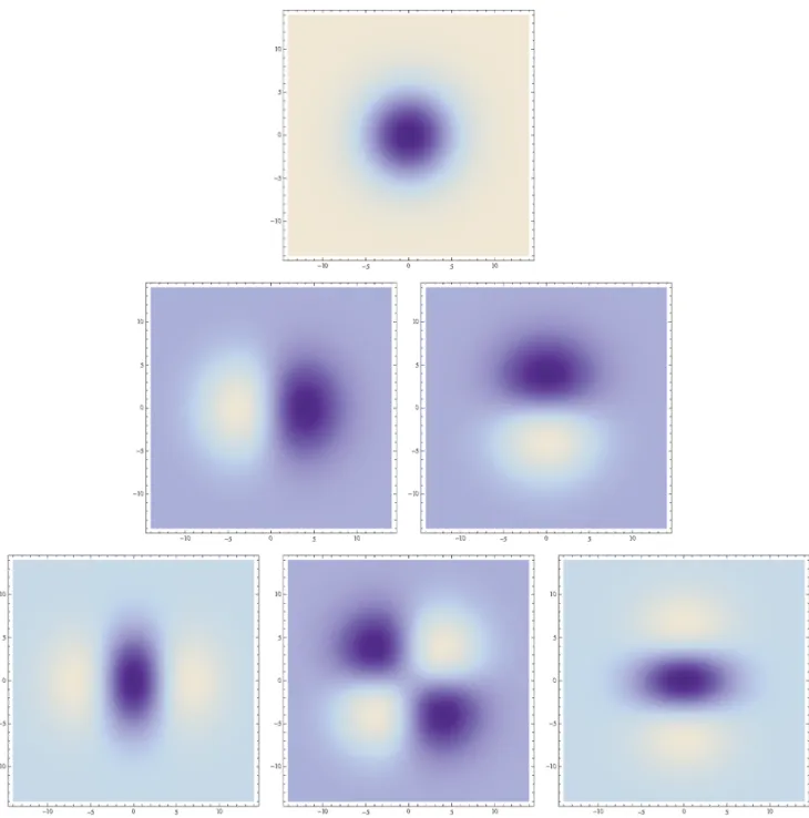
(with a~(a1,a2) wherea1 and a2 denote the order of differen-tiation in the x1- and x2-directions, respectively) as shown in figure 2 with the corresponding one-dimensional Gaussian kernel and its Gaussian derivatives of the form
g g(x1;s)~
1 ffiffiffiffiffiffiffi 2ps
p e{x21=2s, ð26Þ
g
gx1(x1; s)~{
x1
s gg(x1; s)~{ x1 ffiffiffiffiffiffi 2p p
s3=2e
{x21=2s ,
g
gx1x1(x1; s)~ (x2
1{s)
s2 gg(x1; s)~ (x2
1{s) ffiffiffiffiffiffi 2p p
s5=2e
{x21=2s : ð28Þ
Such Gaussian functions have been previously used for modelling biological vision by Koenderink and van Doorn [32,53–55] who proposed the Gaussian derivative model for visual operations and pioneered the modelling of visual operations using differential geometry, by Young [33] who showed that there are receptive fields in the striate cortex that can be well modelled by Gaussian derivatives up to order four, by Lindeberg [56] who extended the Gaussian derivative model for receptive fields with corresponding idealized discretizations and by Petitot [57,58] who expressed a differential geometric model for illusory contours and the singularities in the orientation fields in the primary visual cortex known as pinwheels; see also Sartiet al.[59] for extensions of the latter model to rotations and rescalings of non-Gaussian receptive field profiles.
More generally, these Gaussian derivative operators can be used as ageneral basisfor expressing image operations such as feature detection, feature classification, surface shape, image matching and image-based recognition (Witkin [60]; Koenderink [61]; Koenderink and van Doorn [62]; Lindeberg [63–65]; Florack [66]; ter Haar Romeny [67]); see specifically Schiele and Crowley [68], Linde and Lindeberg [69,70], Lowe [71], and Bayet al.[72] for explicit approaches for object recognition based on Gaussian receptive fields or approximations thereof.
Affine-adapted Gaussian receptive fields. If we relax the requirement of rotational symmetry and relax it into the requirement of mirror symmetry through the origin, then it follows that the convolution kernels must instead beaffine Gaussian kernels(Lindeberg [63])
x
L
Figure 1. The requirement of non-enhancement of local extrema is a way of restricting the class of possible image operations by formalizing the notion that new image structures must not be created with increasing scale, by requiring that the value at a local maximum must not increase and that the value at a local minimum must not decrease.
doi:10.1371/journal.pone.0066990.g001
T(x;s)~g(x; S)~ 1 2p ffiffiffiffiffiffiffiffiffiffiffi
detS
p e{xTS{1x=2
ð29Þ
where S denotes any symmetric positive semi-definite 2|2 matrix. This affine scale-space concept is closed under affine transformations, meaning that if we for affine related images
fL(j)~fR(g) where g~Ajzb, ð30Þ
(which may represent images of a local image patch seen from two
different views, either byLandRrepresenting the left and right views of a binocular observer or L and R representing two different views registered by a monocular observer by translating and/or rotating the object and/or the observer) define corre-sponding scale-space representationsLandRaccording to
L(:;SL)~g(:; SL)fL(:) ð31Þ
R(:; SR)~g(:;SR)fR(:)
Figure 2. Spatial receptive fields formed by the 2-D Gaussian kernel with its partial derivatives up to order two.The corresponding family of receptive fields is closed under translations, rotations and scaling transformations.
doi:10.1371/journal.pone.0066990.g002
then these scale-space representations will be related according to (Lindeberg [63]; Lindeberg and Ga˚rding [40])
L(x; SL)~R(y;SR) ð33Þ
where
SR~ASLAT and y~A xzb: ð34Þ
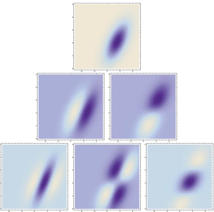
In other words, given that an imagefLis affine transformed into an image fR it will always be possible to find a transformation between the scale parameterssLand sRin the two domains that makes it possible to match the corresponding derived internal representations L(:;sL) and R(:;sR). Figure 3 shows a few examples of such kernels in different directions with the covariance matrix parameterized according to
S ~ l1cos 2hzl
2sin2h (l1{l2) coshsinh (l1{l2) coshsinh l1sin2hzl2cos2h
!
ð35Þ
withl1 and l2 denoting the eigenvalues and hthe orientation. Directional derivatives of these kernels can in turn be obtained from linear combinations of partial derivative operators according to
LQmL ~( cosQLx
1zsinQLx2) mL
~ P m
k~0
m k
coskQsinm{kQL xk1xm{k
2
: ð36Þ
With respect to biological vision, these kernels can be used for modelling receptive fields that are oriented in the spatial domain, as will be described in connection with equation (71) in the section on ‘‘Computational modelling of biological receptive fields’’. For computer vision they can be used for computing affine invariant image descriptorsfore.g.cues to surface shape, image-based matching and recognition (Lindeberg [63]; Lindeberg and Ga˚rding [40]: Baumberg [73]; Mikolajczyk and Schmid [74]; Tuytelaars and van Gool [75]; Lazebniket al.[76]; Rothgangeret al.[77]).
Note on receptive fields formed from derivatives of the convolution kernels. Due to the linearity of the differential equation (23), which has been derived by necessity from the structural requirements, it follows that also the result of applying a linear operatorDto the solutionLwill also satisfy the differential equation, however, with a different initial condition
lim s;0(DL)(
:; s)~Df: ð37Þ
The result of applying a linear operatorD to the scale-space representation L will therefore satisfy the above mentioned structural requirements of linearity, shift invariance, the weaker form of rotational invariance at the group level and non-enhancement of local extrema, with the semi-group structure (6) replaced by the cascade property
(DL)(:;s2)~T(:; s2{s1)(DL)(:; s1): ð38Þ
Then, one may ask if any linear operator D would be reasonable? From the requirement of scale invariance, however, if follows that that the operatorDmust not be allowed to have non-infinitesimal support, since a non-infinitesimal supports0w0 would violate the requirement of self-similarity over scale (9) and it would not be possible to perform image measurements at a scale level lower than s0. Thus, any receptive field operator derived from the scale-space representation in a manner compatible with the structural arguments must correspond to local derivatives. In the illustrations above, partial derivatives and directional deriva-tives up to order two have been shown.
For directional derivatives that have been derived from elongated kernels whose underlying zero-order convolution kernels are not rotationally symmetric, it should be noted that we have aligned the directions of the directional derivative operators to the orientations of the underlying kernels. A structural motivation for making such an alignment can be obtained from a requirement of a weaker form of rotational symmetry at the group level. If we would like the family of receptive fields to be rotationally symmetric as a group, then it is natural to require the directional derivative operators to be transformed in a similar way as the underlying kernels.
Receptive fields in terms of derivatives of the convolution kernels derived by necessity do also have additional advantages if one adds a further structural requirement of invariance under additive intensity transformations f(x).f(x)zC. A zero-order receptive field will be affected by such an intensity transformation, whereas higher order derivatives are invariant under additive intensity transformations. As will be described in the section on ‘‘Invariance property under illumination variations’’, this form of invariance has a particularly interesting physical interpretation with regard to a logarithmic intensity scale.
Spatio-temporal image data
For spatio-temporal image data f(x,t) defined on a 2+12D
spatio-temporal domain with (x,t)~(x1,x2,t) it is natural to inherit the symmetry requirements over the spatial domain. In addition, the following structural requirements can be imposed motivated by the special nature of time and space-time:
Galilean covariance
For time-dependent spatio-temporal image data, we may have
relative motionsbetween objects in the world and the observer, where a constant velocity translational motion can be modelled by a
Galilean transformation
f0~Gvf ð39Þ
corresponding to
f0(x0,t0)~f(x,t) with x0~xzv t: ð40Þ
L0(x0,t0;s0)~L(x,t;s) ð41Þ
corresponding to
TGv(s)Gvf~GvTsf: ð42Þ
Such a property is referred to asGalilean covariance.
Temporal causality. For a vision system that interacts with the environment in a real-time setting, a fundamental constraint
on the convolution kernels (the spatio-temporal receptive fields) is that they cannot access data from the future. Hence, they must be
time-causalin the sense that convolution kernel must be zero for any relative time moment that would imply access to the future:
T(x,t;s)~0 if tv0: ð43Þ
Time-recursivity. Another fundamental constraint on a real-time system is that it cannot keep a record of everything that
Figure 3. Spatial receptive fields formed by affine Gaussian kernels and directional derivatives of these.The corresponding family of receptive fields is closed under general affine transformations of the spatial domain, including translations, rotations, scaling transformations and perspective foreshortening.
has happened in the past. Hence, the computations must be based on a limited internaltemporal bufferM(x,t), which should provide:
N
a sufficient record of past information andN
sufficient information to update its internal state when new information arrives.A particularly useful solution is to use the internal representa-tionsLat different temporal scales also used as the memory buffer of the past. In (Lindeberg [21, section 5.1.3, page 57]) it is shown that such a requirement can be formalized by a time-recursive updating rule of the form
L(x,t2;s2,t)~
~Ð
j[RN Ð
f§0U(x{j,t2{t1;s2{s1,t,f)
L(j,t1; s1,f)dfdj
zÐ
j[RN Ðt2
u~t1B(x{j,t2{u;s2,t)f(j,u)djdu ð44Þ
which is required to hold for any pair of scale levelss2§s1and any two time momentst2§t1, where
N
the kernelU updates the internal state,N
the kernel Bincorporates new image data into the represen-tation,N
tis the temporal scale andfan integration variable referring to internal temporal buffers at different temporal scales.Non-enhancement of local extrema in a time-recursive setting. For a time-recursive spatio-temporal visual front-end it is also natural to generalize the notion of non-enhancement of local extrema, such that it is required to hold both with respect to increasing spatial scales sand evolution over time t. Thus, if at some spatial scales0and time momentt0a point(x0,t0)is a local maximum (minimum) for the mapping
(x,t)?L(x,t0; s0,t) ð45Þ
then for every positive directionu~(u1,. . .,uN,uNz1) in the Nz1 -dimensional space spanned by (s,t), the directional derivative (DuL)(x,t; s,t)must satisfy
(DuL)(x0,t0;s0,t0)ƒ0 at any local maximum, ð46Þ
(DuL)(x0,t0; s0,t0)§0 at any local minimum: ð47Þ
Necessity results concerning spatio-temporal receptive fields
We shall now describe how these structural requirements restrict the class of possible spatio-temporal receptive fields.
Non-causal spatio-temporal receptive fields
If one disregards the requirements of temporal causality and time recursivity and instead requires (i) linearity, (ii) shift invariance over space and time, (iii) semi-group property over spatial and temporal scales, (iv) sufficient regularity properties over space, time and spatio-temporal scales and (v) non-enhancement of local extrema for a multi-parameter scale-space, then it follows from (Lindeberg [21, theorem 5, page 42]) that the scale-space representation over a 2+1-D spatio-temporal domain must satisfy
LsL~1 2+
T
(x,t) S0+(x,t)L
{dT0+(x,t)L ð48Þ
for some3|3covariance matrixS0and some 3-D vectord0with
+(x,t)~(Lx
1,Lx2,Lt) T.
In terms of convolution kernels, the zero-order receptive fields will then bespatio-temporal Gaussian kernels
g(p;Ss,ds)~ 1 (2p)3=2 ffiffiffiffiffiffiffiffiffiffiffiffi
detSs
p e{(p{ds)TSs{1(p{ds)=2s ð49Þ
withp~(x,t)T~(x1,x2,t)T,
Ss ~ f3|3 matrix as shown in table1g ð50Þ
ds ~ v1t
v2t
d
0
B @
1
C A
where (i)l1,l2andhdetermine thespatial extent, (ii)ltdetermines thetemporal extent, (iii)v~(v1,v2)denotes theimage velocityand (iv)d represents atemporal delay. From the correspondingGaussian spatio-temporal scale-space
L(x,t; Sspace,v,t)~(g(:,:; Sspace,v,t)f(:,:))(x,t) ð52Þ
spatio-temporal derivatives can then be defined according to
Lxatb(x,t; Sspace,v,t)~(LxatbL)(x,t; Sspace,v,t) ð53Þ
with corresponding velocity-adapted temporal derivatives
Ltt~vT+xzLt~v1Lx1zv2Lx2zLt ð54Þ
as illustrated in figure 4 and figure 5 for the case of a 1+12D
space-time.
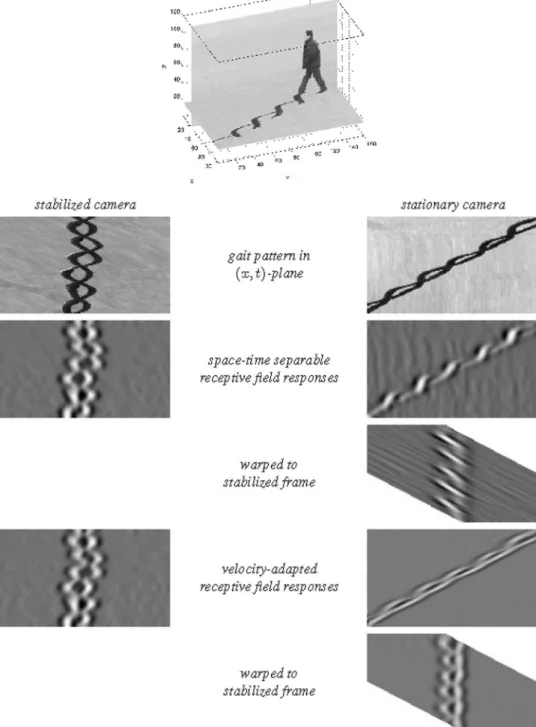
Motivated by the requirement of Galilean covariance, it is natural to align the directions v in space-time for which these velocity-adapted spatio-temporal derivatives are computed to the velocity values used in the underlying zero-order spatio-temporal kernels, since the resulting velocity-adapted spatio-temporal derivatives will then be Galilean covariant. Such receptive fields can be used for modelling spatio-temporal receptive fields in biological vision (Lindeberg [21,56]; Younget al.[34,35]) and for computing spatio-temporal image features and Galilean invariant image descriptors for spatio-temporal recognition in computer
vision (Laptev and Lindeberg [78–80]; Laptevet al.[81]; Willems
et al.[82]).
Transformation property under Galilean
transformations. Under a Galilean transformation of space-time (40), in matrix form written
p0~Gvp ð55Þ
corresponding to
x10
x20
t0
0
B @
1
C
A~
1 0 v1 0 1 v2 0 0 1 0
B B B @
1
C C C A
x1
x2
t 0
B @
1
C
A, ð56Þ
the corresponding Gaussian spatio-temporal representations are related in an algebraically similar way (30–33) as the affine Gaussian scale-space with the affine transformation matrix A replaced by a Galilean transformation matrixGv. In other words, if two spatio-temporal image patternsfL andfRare related by a
Figure 4. Non-causal and space-time separable spatio-temporal receptive fields over 1+12D space-time as generated by the
Gaussian spatio-temporal scale-space model withv~0.This family of receptive fields is closed under rescalings of the spatial and temporal dimensions. (Horizontal axis: spacex. Vertical axis: timet.)
Galilean transformation encompassing a translation
Dp~(Dx1,Dx2,Dt)T in space-time
fL(j)~fR(g) where g~GvjzDp, ð57Þ
(which may represent time-dependent image data registered of an object under different relative motions between the object and the observer) and if corresponding spatio-temporal scale-space repre-sentationsLandRoffL andfRare defined according to
Figure 5. Non-causal and velocity-adapted spatio-temporal receptive fields over 1+1-D space-time as generated by the Gaussian spatio-temporal scale-space model for a non-zero image velocityv. This family of receptive fields is closed under rescalings of the spatial and temporal dimensions as well as Galilean transformations. (Horizontal axis: spacex. Vertical axis: timet.)
doi:10.1371/journal.pone.0066990.g005
Table 1.Spatio-temporal covariance matrix for the Gaussian spatio-temporal scale-space used for modelling non-causal spatio-temporal receptive fields in equation (50).
l1cos2hzl2sin2hzv21lt (l2{l1) coshsinhzv1v2lt v1lt
(l2{l1) coshsinhzv1v2lt l1sin2hzl2cos2hzv22lt v2lt
v1lt v2lt lt
0
B @
1
C A
L(:; SL) ~g(:;SL)fL(:) ð58Þ
R(:; SR) ~g(:;SR)fR(:) ð59Þ
for general spatio-temporal covariance matricesSLandSRof the form (50), then these spatio-temporal scale-space representations will be related according to
L(x; SL)~R(y;SR) ð60Þ
where
SR~GvSLGTv and y~GvxzDp: ð61Þ
Given two spatio-temporal image patterns that are related by a Galilean transformation, such as arising when an object is observed with different relative motion between the object and the viewing direction of the observer, it will therefore be possible to perfectly match the spatio-temporal receptive field responses computed from the different spatio-temporal image patterns. Such a perfect matching would, however, not be possible without velocity adaptation, i.e., if the spatio-temporal receptive fields would be computed using space-time separable receptive fields only.
Time-causal spatio-temporal receptive fields
If we on the other hand with regard to real-time biological vision want to respect both temporal causality and temporal recursivity, we obtain a different family of time-causal spatio-temporal receptive fields. Given the requirements of (i) linearity, (ii) shift invariance over space and time, (iii) temporal causality, (iv) time-recursivity, (v) semi-group property over spatial scalessand timet Ts1,t1Ts2,t2~Ts1zs2,t1zt2, (vi) sufficient regularity properties over space, time and spatio-temporal scales and (vii) non-enhancement of local extrema in a time-recursive setting, then it follows that the time-causal spatio-temporal scale-space must satisfy thesystemof diffusion equations (Lindeberg [21, equations (88–89), page 52, theorem 17, page 78])
LsL ~1 2+
T
x(S+xL) ð62Þ
LtL ~{vT+ xLz
1
2LttL ð63Þ
for some 2|2 spatial covariance matrix S and some image velocityvwithsdenoting thespatial scaleandtthetemporal scale. In terms of receptive fields, this spatio-temporal scale-space can be computed by convolution kernels of the form
h(x,t; s,t;S,v)~g(x{vt;s; S)w(t; t)~
~ 1
2ps ffiffiffiffiffiffiffiffiffiffiffi detS
p e{(x{vt)TS{1(x{vt)=2s 1
ffiffiffiffiffiffi 2p p
t3=2te
{t2=2t ð64Þ
where
N
g(x{vt;s; S)is avelocity-adapted 2-D affine Gaussian kernelwith covariance matrixSandN
w(t; t) is a time-causal smoothing kernel over time with temporal scale parametert.From these kernels, spatio-temporal partial derivatives and velocity-adapted derivatives can be computed in a corresponding manner (53) and (54) as for the Gaussian spatio-temporal scale-space concept; see figure 6 and figure 7 for illustrations in the case of a 1+12D space-time.
Concerning the relations between the non-causal spatio-temporal model in section "Non-causal spatio-spatio-temporal receptive fields", and the time-causal model in section ‘‘Time-causal spatio-temporal receptive fields’’, please note that requirement of non-enhancement of local extrema is formulated in different ways in the two cases: (i) For the non-causal scale-space model, the condition about non-enhancement condition is based on points that are local extrema with respect to both spacexand timet. At such points, a sign condition is imposed on the derivative in any positive direction over spatial scalessand temporal scalet. (ii) For the time-causal scale-space model, the notion of local extrema is based on points that are local extrema with respect to spacexand the internal temporal buffers at different temporal scalest. At such points, a sign condition is imposed on the derivatives in the parameter space defined by the spatial scale parameterssand time t. Thus, in addition to the restriction to time-causal convolution kernels (43) the derivation of the time-causal scale-space model is also based on different structural requirements.
Other time-causal temporal scale-space models have been proposed by Koenderink [83] based on a logarithmic transfor-mation of time in relation to a time delay relative to the present moment and by Lindeberg and Fagerstro¨m [84] based on a set of first-order integrators corresponding to truncated exponential filters with time constantsmicoupled in cascade
hcomposed(t; m)~ki~1 1
mie
{t=mi ð65Þ
with the composed kernel having temporal variance
tk~ Xk
t~1
m2
i: ð66Þ
Such first-order temporal integrators satisfy weaker scale-space properties in the sense of guaranteeing non-creation of local extrema or zero-crossings for a one-dimensional temporal signal, although they do not permit true covariance under rescalings of the temporal axis. Moreover, they are inherently time recursive and obey a temporal update rule between adjacent temporal scale levelstk{1andtkof the following form:
LtL(t; tk)~ 1
mk
L(t; tk{1){L(t;tk)
Such kernels can also be used as an idealized computational model for temporal processing in biological neurons (Koch [85, Chapters 11–12]). If we combine these purely temporal smoothing kernels with the general form of spatio-temporal kernels
Tspace{time(x,t;s,t; S,v)~
~g(x{vt; s; S)Ttime(t; t) ð68Þ
as obtained from a principled treatment over the joint space-time domain, we obtain an additional class of causal and time-recursive spatio-temporal receptive fields with the additional restrictions that the temporal scale parameter has to be discretized already in the theory and that temporal covariance cannot hold
Figure 6. Time-causal and space-time separable spatio-temporal receptive fields over a 1+12D space-time as generated by the
time-causal spatio-temporal scale-space model withv~0.This family of receptive fields is closed under rescalings of the spatial and temporal dimensions. (Horizontal axis: spacex. Vertical axis: timet.)
exactly for temporal scale levels that have been determined beforehand. For the logarithmic scale-time approach by Koender-ink [83], there is, however, not any known time-recursive implementation suitable for real-time processing.
Computational modelling of biological receptive fields
An attractive property of the presented framework for early receptive fields is that it generates receptive field profiles in good
Figure 7. Time-causal and velocity-adapted spatio-temporal receptive fields over a 1+12D space-time as generated by the
time-causal spatio-temporal scale-space model withv~0. This family of receptive fields is closed under rescalings of the spatial and temporal dimensions as well as Galilean transformations. (Horizontal axis: spacex. Vertical axis: timet.)
agreement with receptive field profiles found by cell recordings in the retina, LGN and V1 of higher mammals. DeAngeliset al.[26] and DeAngelis and Anzai [27] present overviews of (classical) receptive fields in the joint space-time domain. As outlined in (Lindeberg [21, section 6]), the Gaussian and time-causal scale-space concepts presented here can be used for generating predictions of receptive field profiles that are qualitatively very similar to all the spatial and spatio-temporal receptive fields presented in these surveys.
LGN neurons
In the LGN, most cells (i) have approximately circular-center surround and most receptive fields are (ii) space-time separable
(DeAngeliset al.[26]; DeAngelis and Anzai [27]). A corresponding idealized scale-space model for such receptive fields can be expressed as
hLGN(x1,x2,t;s,t)~
+(Lx
1x1zLx2x2)g(x1,x2;s)Lt0nh(t; t)
ð69Þ
where
N
+ determines the polarity (on-center/off-surround vs: off-center/on-surround),N
Lx1x1zLx2x2 denotes the spatial Laplacian operator,N
g(x1,x2;s)denotes a rotationally symmetric spatial Gaussian,N
Lt0 denotes a temporal derivative operator with respect to a possibly self-similar transformation of timet0~taort0~logt such thatLt0~tkLtfor some constantk[21, section 5.1, pages 59–61],N
h(t; t)is a temporal smoothing kernel over time corresponding to the time-causal smoothing kernelw(t; t)~ 1ffiffiffiffiffiffi
2p p
t3=2te
{t2=2t
in (64) or a non-causal time-shifted Gaussian kernel
g(t; t,d)~ ffiffiffiffiffiffiffiffi1 2pt
p e{(t{d)2=2t
according to (49), alternatively a
time-causal kernel of the form (65) corresponding to a set of first-order integrators over time coupled in cascade,
N
nis the order of temporal differentiation,N
sis the spatial scale parameter andN
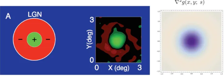
tis the temporal scale parameter.Figure 8 shows a comparison between the spatial component of a receptive field in the LGN with a Laplacian of the Gaussian. This model can also be used for modelling on-center/off-surround and off-center/on-surround receptive fields in the retina.
Regarding the spatial domain, the model in terms of spatial Laplacians of Gaussians(Lx1x1zLx2x2)g(x1,x2; s)is closely related
to differences of Gaussians, which have previously been shown to be good approximation of the spatial variation of receptive fields in the retina and the LGN (Rodieck [31]). This property follows from the fact that the rotationally symmetric Gaussian satisfies the isotropic diffusion equation
1 2+
2L(x
;t) ~LtL(x;t)
&L(x; tzDt){L(x; t)
Dt
~DOG(x; t,Dt)
Dt ð70Þ
which implies that differences of Gaussians can be interpreted as approximations of derivatives over scale and hence to Laplacian responses.
Simple cells in V1
In V1 the receptive fields are generally different from the receptive fields in the LGN in the sense that they are (i)oriented in the spatial domainand (ii)sensitive to specific stimulus velocities(DeAngelis
et al.[26]; DeAngelis and Anzai [27]).
Spatial dependencies
We can express a scale-space model for thespatial componentof this orientation dependency according to
hspace(x1,x2; s)~( cosQLx1zsinQLx2)mg(x1,x2; S) ð71Þ
where
N
LQ~cosQLx1zsinQLx2 is a directional derivative operator,N
mis the order of spatial differentiation andN
g(x1,x2; S) is an affine Gaussian kernel with spatial covariance matrixSas can be parameterized according to (35)where the directionQof the directional derivative operator should preferably be aligned to the orientation h of one of the eigenvectors of S. Figure 9 shows a comparison between this idealized receptive field model over the spatial domain and the spatial response properties of a simple cell in V1.
In the specific case when the covariance matrix is proportional to a unit matrix S~s I, with s denoting the spatial scale parameter, these directional derivatives correspond to regular Gaussian derivatives as proposed as a model for spatial receptive fields by Koenderink and van Doorn [32,62]. The use of non-isotropic covariance matrices does on the other hand allow for a higher degree of orientation selectivity. Moreover, by having a family of affine adapted kernels tuned to a family of covariance matrices with different orientations and different ratios between the scale parameters in the two directions, the family as a whole can represent affine covariance which makes it possible to perfectly match corresponding receptive field responses between different views obtained under variations of the viewing direction in relation to the object.
Figure 10 shows illustrations of affine receptive fields of different orientations and degrees of elongation as they arise if we assume that the set of all 3-D objects in the world have an approximately uniform distribution of surface orientations in 3-D space and if we furthermore assume that we observe these objects from a uniform distribution of viewing directions that are not directly coupled to properties of the objects.
This idealized model of elongated receptive fields can also be extended to recurrent intracortical feedback mechanisms as formulated by Somerset al. [86] and Sompolinsky and Shapley [87] by starting from the equivalent formulation in terms of the non-isotropic diffusion equation (23)
LsL~1 2+
T
xðS0+xLÞ ð72Þ
image data in a neighbourhood of each image point; see Weickert [88] and Almansa and Lindeberg [89] for applications of this idea to the enhancement of local directional image structures in computer vision.
By the use of locally adapted feedback, the resulting evolution equation does not obey the original linearity and shift-invariance (homogeneity) requirements used for deriving the idealized affine Gaussian receptive field model, if the covariance matricesS0are determined from a properties of the image data that are determined in a non-linear way. For a fixed set of covariance matricesS0at any image point, the evolution equation will still be linear and will specifically obey non-enhancement of local extrema. In this respect, the resulting model could be regarded as a simplest form of non-linear extension of the idealized receptive field model.
Relations to modelling by Gabor functions. Gabor functions have been frequently used for modelling spatial receptive fields (Marcˇelja [28]; Jones and Palmer [29,30]), motivated by their property of minimizing the uncertainty relation. This
motivation can, however, be questioned on both theoretical and empirical grounds. Stork and Wilson [90] argue that (i) only complex-valued Gabor functions that cannot describe single receptive field minimize the uncertainty relation, (ii) the real functions that minimize this relation are Gaussian derivatives rather than Gabor functions and (iii) comparisons among Gabor and alternative fits to both psychophysical and physiological data have shown that in many cases other functions (including Gaussian derivatives) provide better fits than Gabor functions do.
Conceptually, the ripples of the Gabor functions, which are given by complex sine waves, are related to the ripples of Gaussian derivatives, which are given by Hermite functions. A Gabor function, however, requires the specification of a scale parameter and a frequency, whereas a Gaussian derivative requires a scale parameter and the order of differentiation. With the Gaussian derivative model, receptive fields of different orders can be mutually related by derivative operations, and be computed from each other by nearest-neighbour operations. The zero-order receptive fields as well as the derivative based receptive fields
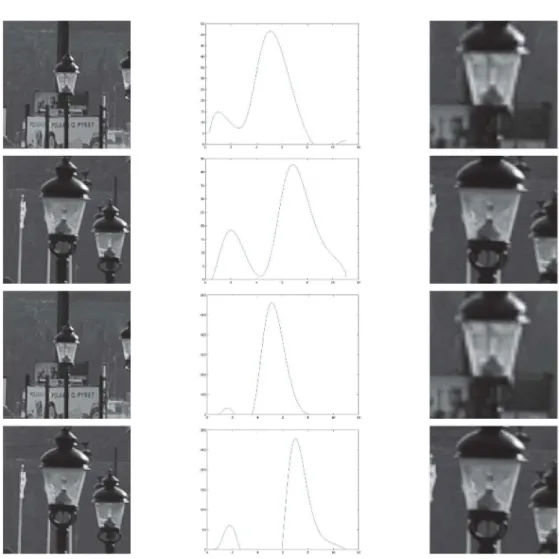
Figure 8. Spatial component of receptive fields in the LGN.(left) Receptive fields in the LGN have approximately circular center-surround responses in the spatial domain, as reported by DeAngeliset al.[26]. (right) In terms of Gaussian derivatives, this spatial response profile can be modelled by the Laplacian of the Gaussian+2g(x,y; s)~(x2zy2{2s)=(2ps3) exp ({(x2zy2)=2s), here withs~0:35deg2.
doi:10.1371/journal.pone.0066990.g008
Figure 9. Spatial component of receptive fields in V1.(left) Simple cells in the striate cortex do usually have strong directional preference in the spatial domain, as reported by DeAngeliset al.[26]. (right) In terms of Gaussian derivatives, first-order directional derivatives of anisotropic affine Gaussian kernels, here aligned to the coordinate directionsLxg(x,y; S)~Lxg(x,y;lx,ly)~{x
lx
1=(2p ffiffiffiffiffiffiffiffiffi
lxly
p
) exp ({x=2lx{y2=2ly)and here with
lx~0:2deg2andly~1:9deg2, can be used as a model for simple cells with a strong directional preference.
can be modelled by diffusion equations, and can therefore be implemented by computations between neighbouring computa-tional units.
In relation to invariance properties, the family of affine Gaussian kernels is closed under affine image deformations, whereas the family of Gabor functions obtained by multiplying rotationally symmetric Gaussians with sine and cosine waves is not closed under affine image deformations. This means that it is not possibly to compute truly affine invariant image representations from such Gabor functions. Instead, given a pair of images that are related by a non-uniform image deformation, the lack of affine covariance implies that there will be a systematic bias in image representations derived from such Gabor functions, corresponding to the difference between the backprojected Gabor functions in the two image domains. If using receptive profiles defined from directional derivatives of affine Gaussian kernels, it will on the other hand be possible to compute affine invariant image representations.
In this respect, the Gaussian derivative model can be regarded as simpler, it can be related to image measurements by differential geometry, be derived axiomatically from symmetry principles, be computed from a minimal set of connections and allows for provable invariance properties under non-uniform (affine) image deformations. Young [33] has more generally shown that spatial receptive fields in cats and monkeys can be well modelled by Gaussian derivatives up to order four.
Spatio-temporal dependencies
To model spatio-temporal receptive fields in thejoint space-time domain, we can then state scale-space models of simple cells in V1 using either
N
non-causal Gaussian spatio-temporal derivative kernelshGaussian(x1,x2,t;s,t,v,d)~
~(La1
Q La\2QLttng)(x1,x2,t; s,t,v,d) ð73Þ
N
time-causal spatio-temporal derivative kernelshtime{causal(x1,x2,t; s,t,v)~
~(L
xa1 1 x
a2
2
Lttnh)(x1,x2,t; s,t,v)
ð74Þ
with the non-causal Gaussian spatio-temporal kernels g(x1,x2,t;s,t,v,d) according to (49), the time-causal spatio-temporal kernels h(x1,x2,t;s,t,v) according to (64) and spatio-temporal derivatives L
xa1 1 x
a2
2
L
tb or velocity-adapted derivatives
L
xa11xa22Lttb of these according to (53) and (54).
For a general orientation of receptive fields with respect to the spatial coordinate systems, the receptive fields in these scale-space models can be jointly described in the form
hsimple{cell(x1,x2,t; s,t,v,S)~
~( cosQLx
1zsinQLx2)
a1( sinQL
x1{cosQLx2)a2
(v1Lx1zv2Lx2zLt)n
g(x1{v1t,x2{v2t;sS)h(t; t) ð75Þ
where
N
LQ~cosQLx1zsinQLx2 and L\Q~sinQLx1{cosQLx2 de-note spatial directional derivative operators according to (36) in two orthogonal directionsQand\Q,N
a1§0anda2§0denote the orders of differentiation in the two orthogonal directions in the spatial domain with the overall spatial order of differentiationm~a1za2,N
v1Lx1zv2Lx2zLt denotes a velocity-adapted temporal deriv-ative operator,N
v~(v1,v2)denotes the image velocity,Figure 10. Affine Gaussian receptive fields generated for a set of covariance matricesSthat correspond to an approximately uniform distribution on a hemisphere in the 3-D environment, which is then projected onto a 2-D image plane.(left) Zero-order receptive fields. (right) First-order receptive fields.
N
ndenotes the order of temporal differentiation,N
g(x1{v1t,x2{v2t;S)denotes a spatial affine Gaussian kernel according to (29) that translates with image velocityv~(v1,v2) in space-time,N
Sdenotes a spatial covariance matrix that can be parameter-ized by two eigenvaluesl1andl2as well as an orientationhof the form (35),N
h(t; t)is a temporal smoothing kernel over time corresponding to the time-causal smoothing kernelQ(t; t)~ ffiffiffiffiffiffi12p p
t3=2te
{t2=2t
in (64) or a non-causal time-shifted Gaussian kernel
g(t; t,d)~ 1
ffiffiffiffiffiffiffiffi
2pt
p e{(t{d)2=2t
according to (49), alternatively a
time-causal kernel of the form (65) corresponding to a set of first-order integrators over time coupled in cascade,
N
sdenotes the spatial scale andN
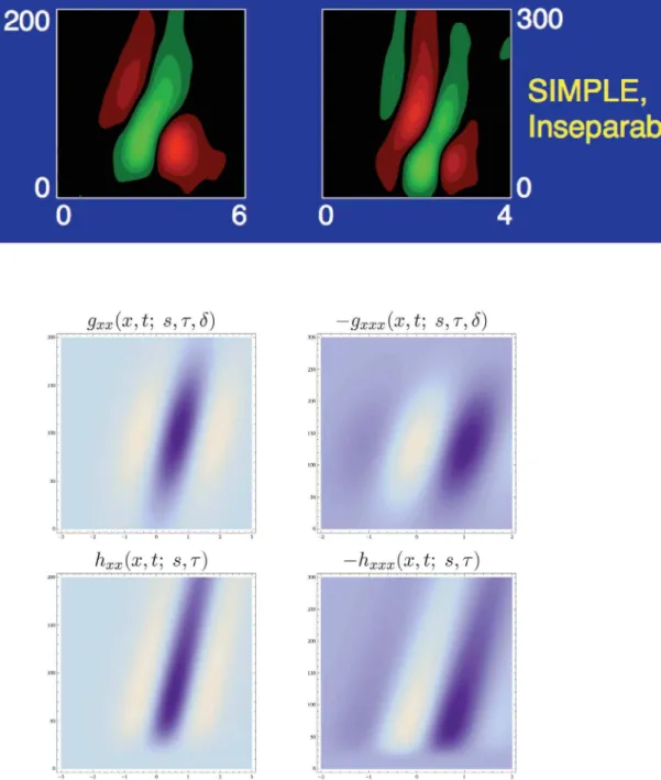
tdenotes the temporal scale.Figure 11 shows examples of non-separable spatio-temporal receptive fields measured by cell recordings in V1 with corresponding velocity-adapted spatio-temporal receptive fields obtained using the Gaussian space and the time-causal scale-space; see also Younget al.[34] and Young and Lesperance [35] for a closely related approach based on Gaussian spatio-temporal derivatives although using a different type of parameterization and Lindeberg [56] for closely related earlier work. These scale-space models should be regarded asidealized functional and phenomenological models of receptive fields that predict how computations occur in a visual system and whose actual realization can then be implemented in different ways depending on available hardware or wetware.
Work has also been performed on learning receptive field properties and visual models from the statistics of natural image data (Field [44]; van der Schaaf and van Hateren [45]; Olshausen and Field [46]; Rao and Ballard [47]; Simoncelli and Olshausen [48]; Geisler [49]) and been shown to lead to the formation of similar receptive fields as found in biological vision. The proposed theoretical model on the other hand makes it possible to determine such receptive fields from theoretical first principles that reflect symmetry properties of the environment and thus without need for any explicit training stage or selection of representative image data. This normative approach can therefore be seen as describing the solution that an idealized learning based system may converge to, if exposed to a sufficiently large and representative set of natural image data.
An interesting observation that can be made from the similarities between the receptive field families derived by necessity from the assumptions and receptive profiles found by cell recordings in biological vision, is that receptive fields in the retina, LGN and V1 of higher mammals are very close toidealin view of the stated structural requirements/symmetry properties (Linde-berg [22]). In this sense, biological vision can be seen as having adapted very well to the transformation properties of the outside world and the transformations that occur when a three-dimen-sional world is projected to a two-dimenthree-dimen-sional image domain.
Mechanisms for obtaining true geometric invariances
An important property of the above mentioned families of spatial and spatio-temporal receptive fields is that they obey basic
covariance propertiesunder
N
rescalingsof the spatial and temporal dimensions,N
affine transformationsof the spatial domain andN
Galilean transformations of space-time;see (Lindeberg [21, section 5.1.2, page 56]) for more precise statements and explicit equations. These properties do in turn allow the vision system to handle:
N
image data acquired with different spatial and temporal sampling rates, including image data that are sampled with differentspatial resolutionon a foveated sensor with decreasing sampling rate towards the periphery and spatio-temporal events that occur atdifferent speed(fastvs.slow),N
image structures of different spatial and/or temporal extent, including objects of differentsizein the world and events with longer or shorterdurationover time,N
objects at differentdistancesfrom the camera,N
the linear component ofperspective deformations(e.g.perspective foreshortening) corresponding to objects or events viewed from different viewing directions andN
the linear component of relative motions between objects or events in the world and the observer.In these respects, the presented receptive field models ensure that visual representations will bewell-behavedunderbasic geometric transformationsin the image formation process.
This framework can then in turn be used as a basis for defining
truly invariant representations. In the following, we shall describe basic approaches for this that have been developed in the area of computer vision, and have been demonstrated to be powerful mechanisms for achieving scale invariance, affine invariance and Galilean invariance for real-world data. Since these mechanisms are expressed at a functional level of receptive fields, we propose that corresponding mechanisms can be applied to neural models and a for providing a mathematically well-founded framework for explaining invariance properties in computational models.
Scale invariance
Given a set of receptive fields that operate over some range of scale, a general approach for obtaining scale invariance is by performing scale selection from local extrema over scale of scale-normalized derivatives(Lindeberg [39,63])
Lj
1~s
c=2L
x1 Lj2~sc=2Lx
2 ð76Þ
wherec[½0,1is a free parameter that can be adjusted to the task and in some cases be chosen asc~1. Specifically, it can be shown that if a spatial imagef(x)has a local extremum over scale at scale s0for some positionx0in image space, then if we define a rescaled imagef0(x0)byf0(x0)~f(x)wherex0~axfor some scaling factor