www.atmos-chem-phys.net/14/913/2014/ doi:10.5194/acp-14-913-2014
© Author(s) 2014. CC Attribution 3.0 License.
Chemistry
and Physics
A global climatology of stratosphere–troposphere exchange using
the ERA-Interim data set from 1979 to 2011
B. Škerlak, M. Sprenger, and H. Wernli
ETH Zurich, IAC, Universitätstrasse 16, 8092 Zürich, Switzerland
Correspondence to:B. Škerlak ([email protected])
Received: 15 March 2013 – Published in Atmos. Chem. Phys. Discuss.: 2 May 2013 Revised: 21 September 2013 – Accepted: 11 December 2013 – Published: 27 January 2014
Abstract. In this study we use the ERA-Interim reanaly-sis data set from the European Centre for Medium-Range Weather Forecasts (ECMWF) and a refined version of a previously developed Lagrangian methodology to compile a global 33 yr climatology of stratosphere–troposphere ex-change (STE) from 1979 to 2011. Fluxes of mass and ozone are calculated across the tropopause, pressure surfaces in the troposphere, and the top of the planetary boundary layer (PBL). This climatology provides a state-of-the-art quantifi-cation of the geographical distribution of STE and the pre-ferred transport pathways, as well as insight into the temporal evolution of STE during the last 33 yr.
We confirm the distinct zonal and seasonal asymmetry found in previous studies using comparable methods. The subset of “deep STE”, where stratospheric air reaches the PBL within 4 days or vice versa, shows especially strong ge-ographical and seasonal variations. The global hotspots for deep STE are found along the west coast of North America and over the Tibetan Plateau, especially in boreal winter and spring. An analysis of the time series reveals significant pos-itive trends of the net downward mass flux and of deep STE in both directions, which are particularly large over North America.
The downward ozone flux across the tropopause is dom-inated by the seasonal cycle of ozone concentrations at the tropopause and peaks in summer, when the mass flux is nearly at its minimum. For the subset of deep STE events, the situation is reversed and the downward ozone flux into the PBL is dominated by the mass flux and peaks in early spring. Thus surface ozone concentration along the west coast of North America and around the Tibetan Plateau are likely to be influenced by deep stratospheric intrusions.
We discuss the sensitivity of our results on the choice of the control surface representing the tropopause, the horizon-tal and vertical resolution of the trajectory starting grid, and the minimum residence timeτused to filter out transient STE
trajectories.
1 Introduction
Stratosphere–troposphere exchange (STE) has important im-pacts on atmospheric chemistry: it changes the oxidative ca-pacity of the troposphere (e.g. Kentarchos and Roelofs, 2003) and potentially also affects the climate system because ozone and water vapour are potent greenhouse gases (e.g. Gauss et al., 2003; Forster et al., 2007).
Although it has been known for roughly 50 yr that strato-spheric ozone can be brought into the troposphere during STE events (Junge, 1962; Danielsen, 1968) and add to local photochemical production, the relative importance of these sources is not yet entirely certain. Modelling studies (e.g. Roelofs and Lelieveld, 1997) indicate that the stratospheric contribution to ozone in the troposphere could be as large as that from net photochemical production, which was also confirmed in a more recent multi-model ensemble simula-tion (Stevenson et al., 2006). This contribusimula-tion, albeit only known with rather large uncertainty (Wild, 2007), is likely to increase over the next decades (Zeng and Pyle, 2003; Collins et al., 2003; Hegglin and Shepherd, 2009), which further em-phasizes the importance of STE for tropospheric chemistry.
(e.g. Lippmann, 1989; Knowlton et al., 2004). It is therefore not only important to quantify the global net ozone flux across the tropopause but also to investigate the transport and mixing after the crossing (e.g. Bourqui and Trepanier, 2010). The question of where and how often stratospheric in-trusions can reach the planetary boundary layer and to what extent STE contributes to total ozone levels at the surface is a topic of ongoing research (e.g. Davies and Schuepbach, 1994; Stohl et al., 2000; Vingarzan, 2004; Cooper et al., 2005; Trickl et al., 2010; Cristofanelli et al., 2010; Lefohn et al., 2011, 2012; Kuang et al., 2012; Lin et al., 2012).
The current study provides a global climatology of STE from 1979 to 2011 based on a refined version of the La-grangian method introduced by Wernli and Bourqui (2002) and the state-of-the-art reanalysis data set ERA-Interim from the European Centre for Medium-Range Weather Forecasts (ECMWF). This methodology allows for study of the trans-port pathways from the stratosphere to the troposphere (STT) and from the troposphere to the stratosphere (TST). Of par-ticular interest are so-called “deep” exchange events where stratospheric air, which typically is rich in ozone, reaches the planetary boundary layer (PBL) (deep STT) or poten-tially polluted air from the PBL is rapidly transported into the stratosphere (deep TST).
Climatologies using meteorological data with a spatial and temporal resolution high enough to capture important synoptic systems (e.g. Sprenger and Wernli, 2003; James et al., 2003b) nicely complement global-scale estimates (e.g. Holton et al., 1995) and synoptic-scale modelling case stud-ies (e.g. Lamarque and Hess, 1994; Bourqui, 2006). The La-grangian method used in this study also has several advan-tages over other methods such as the budget approach (Ap-penzeller et al., 1996), which does not allow for study of the transport pathways; the Eulerian Wei method (Wei, 1987), which additionally suffers from errors due to the cancellation of large terms (Wirth and Egger, 1999) and large sensitivity to errors in the input fields (Gettelman and Sobel, 2000); and isentropic trajectory calculations (Seo and Bowman, 2001), which are frequently limited to a few isentropes and thus miss a significant amount of exchange events (Sprenger and Wernli, 2003). A good overview of previous climatologies of STE, the methods used, and their limitations is given in the review paper of Stohl et al. (2003) and the studies of Wirth and Egger (1999) and Wernli and Bourqui (2002).
The tropopause definition used in our study is the combination of the ±2 pvu potential vorticity (PV)
(Er-tel, 1942) isosurfaces and the 380 K isentrope, which is a well-established definition for the dynamical tropopause (Hoskins et al., 1985; Holton et al., 1995) (1 pvu=
10−6K m2kg−1s−1). Since PV is conserved in adiabatic, frictionless flow, the dynamical tropopause is a generally well-defined continuous surface with a quasi-material char-acter. Air parcels can only cross the dynamical tropopause if diabatic or other non-conservative processes such as friction change the PV (or the potential temperature2in the
trop-ics). This definition captures the complex, three-dimensional structure of the tropopause which is often observed near jet streams, cyclones, and cut-off lows (e.g. Bithell et al., 1999) and enables the calculation of cross-tropopause fluxes in situations when other control surfaces such as the lapse-rate tropopause are discontinuous. Many other tropopause definitions exist (e.g. Hoinka, 1997), and evidently, fluxes across a control surface crucially depend on its definition (see Sect. 5).
This paper is structured as follows: we first describe the data set and the methodology in Sect. 2. Then we present the climatology of the cross-tropopause mass flux in Sect. 3, followed by the results for the cross-tropopause ozone flux in Sect. 4. The sensitivity of our results to various parame-ters and the choice of control surface is explored in Sect. 5. In Sect. 6, we discuss caveats of the methodology, compare our results to the findings of Sprenger and Wernli (2003) and other studies, and elaborate some regional aspects. Finally, we present our conclusions in Sect. 7.
2 Data and methodology
2.1 Overview
The reanalysis data set ERA-Interim from the ECMWF (Simmons et al., 2006; Dee et al., 2011) is continuously up-dated and covers the time from 1 January 1979 to the present day. Our analysis covers the first 33 yr from 1979 up to and including 2011. The primary analysis fields (e.g. wind and temperature) were interpolated on a regular grid with 1◦
hor-izontal resolution and the secondary fields such as2and PV
were then calculated on the original hybrid model levels as described in Sprenger and Wernli (2003). The Lagrangian methodology presented in Wernli and Bourqui (2002) and applied to the ERA-15 data set in Sprenger and Wernli (2003) was further developed and used to calculate mass and ozone fluxes across the tropopause, pressure surfaces in the middle and lower troposphere (500, 600, 700, and 800 hPa) and the top of the PBL.
This methodology is based on a large set of trajectories started every 24 h on a regular grid spanning the whole globe between 650 and 50 hPa. The spacing of this grid is approxi-mately1x=80 km in the horizontal and1p=30 hPa in the
vertical. In the tropics (between 30◦S and 30◦N) the
verti-cal grid spacing is 10 hPa to accommodate for the typiverti-cally slower vertical motion. The kinematic trajectories are calcu-lated with the tool developed by Wernli and Davies (1997) using the three-dimensional wind fields from ERA-Interim.
Only trajectories that cross the tropopause (2 pvu/380 K) within the first 24 h are selected, and these are extended for 4 days forward and backward, resulting in a total length of 9 days. To remove trajectories representing transient ex-changes, a two-way minimum residence time (τ) criterion is
least τ=48 h on one side of the tropopause before
cross-ing and then remain on the other side for at least 48 h. Thus, only “significant” exchange events are taken into account. Each trajectory represents a fixed amount of mass given by the spacing of the starting grid:1m≈1g(1x)21p≈6.52×
1011kg (in the extratropics). The mass flux across a sur-face is thus calculated by counting the number of crossing trajectories and multiplying by 1m. Note that trajectories
started in the tropics have a smaller1pand thus a smaller 1m. The STT ozone flux is calculated accordingly with 1mO3≈
MO3
Md ·1m· [O3], whereMO3 andMdrepresent the
molecular weights of ozone and dry air, respectively. The ozone concentration at the crossing,[O3], is obtained from
linear spatial and temporal interpolation to the trajectory lo-cation.
The two main enhancements of this methodology intro-duced in the current study are a more elaborated distinction between the troposphere and the stratosphere using a 3-D la-belling algorithm and an altered definition of vertically deep exchange events, which is more relevant for understanding surface ozone concentrations.
2.2 3-D labelling
Outside the tropics, an STE event can in principle be detected as a transition of the trajectory’s PV from below to above 2 pvu (−2 pvu in the Southern Hemisphere) or vice versa.
However, there are diabatically produced PV structures in the troposphere and low-level PV anomalies due to friction, for instance near mountains. If their PV value exceeds 2 pvu, they may be mistaken as stratospheric air. We have there-fore used a refined version of the 3-D labelling algorithm in-troduced in Sprenger et al. (2003) to separate tropospheric and stratospheric air more objectively. This algorithm not only combines the±2 pvu and the 380 K criterion but also
checks the connectivity of grid points with|PV|>2 pvu to
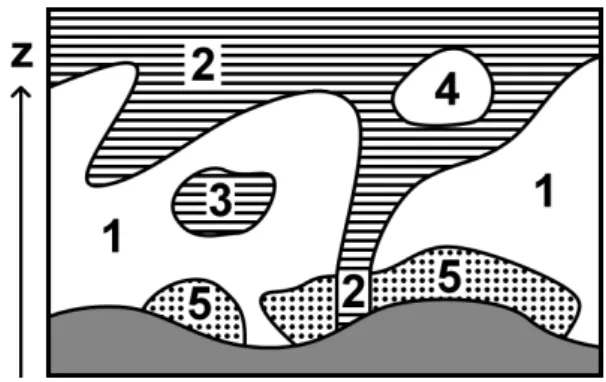
the stratosphere or the surface and assigns labels from 1 to 5 to every grid point, as illustrated in Fig. 1. The label 2 (strato-sphere) is initialized above 380 K and iteratively given to all horizontally, vertically, or diagonally connected grid points with |PV|>2 pvu. Analogously, the label 1 (troposphere)
is initialized at the lowest model level at all points where
|PV|<2 pvu and distributed to all connected grid points.
Grid points with |PV|>2 pvu which were not reached by
the label 2 are assigned the label 3 (three-dimensional strato-spheric cut-offs or diabatically produced PV anomalies) and analogous for tropospheric cut-offs (label 4). STE events are thus identified as transitions from label 2 to 1 (STT) and 1 to 2 (TST) within 24 h.
Over Greenland and especially over Antarctica, very sta-ble air masses just above the surface often have high PV val-ues. Because these PV anomalies are of different nature than stratospheric cut-offs, they are assigned a separate label 5, which is initialized at all grid points on the lowest model
Fig. 1.The 3-D labelling algorithm assigns labels from 1 to 5 to
ev-ery grid point based on PV,2, and the “connectivity” to the top
of the ERA-Interim data set or the surface. The labels used are as follows: 1, troposphere; 2, stratosphere; 3, stratospheric cut-off in the troposphere or other cyclonic PV anomaly not connected to the stratosphere; 4, tropospheric cut-off in the stratosphere; and 5, surface-bound PV anomaly. In the special cases where label 2 merges with label 5, the label 2 is attributed to grid points in the vertical column below the area of contact. The label 2 can only propagate horizontally if the contact occurs in the upper half of the troposphere (in this vertical column). See Sect. 2.2 for a more de-tailed description of this algorithm.
level with|PV|>2 pvu. If such a surface-bound PV anomaly
comes in contact with a low tropopause, distinguishing be-tween the anomaly and the stratosphere requires an addi-tional criterion. Instead of the threshold in specific humidity chosen by Sprenger et al. (2003) and Gray (2003), which is problematic in the case of very dry air masses above Antarc-tica, our new criterion is of geometric nature. We impose that label 2 can always propagate vertically and overrides label 5. As a consequence, all grid points with |PV|>2 pvu in the
vertical column below an area of contact between label 2 and label 5 are given the label 2. The horizontal propagation of label 2 in such cases, however, is limited to the upper half of the troposphere (calculated for every column) which pre-vents the label 2 from being spread over a large area near the surface. The very few cases where a trajectory originat-ing within a surface-bound PV anomaly (label 5) meets such a “stratospheric funnel” (label 2) and then enters the tropo-sphere (label 1) are filtered out by requiring that the label remain constant along the trajectory for 48 h before and after the tropopause crossing.
2.3 Deep exchange events
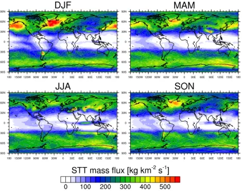
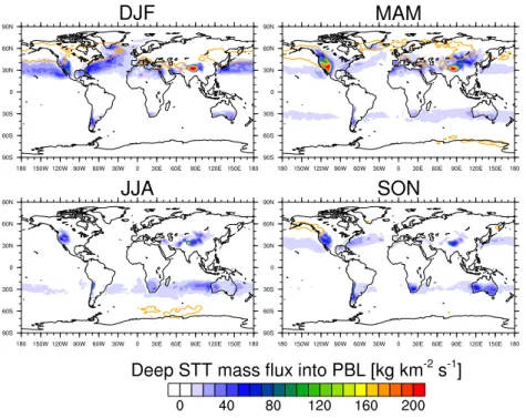
Fig. 2.Seasonally averaged STT mass flux for 1979–2011 (DJF: December, January, February; MAM: March, April, May; JJA: June, July, August; SON: September, October, November).
a minimum height lower than 3 km (James et al., 2003b). These are crude approximations to the PBL height, which ignore its diurnal cycle and geographical variation and limit the investigation to areas without high topography. There-fore, in this study, we use the PBL height from ERA-Interim 6-hourly forecasts to identify deep exchange events. A tra-jectory is thus only selected as a deep exchange if its pres-sure exceeds the prespres-sure at the PBL top at any time step af-ter the exchange (for deep STT) or before the exchange (for deep TST). If multiple crossings of the PBL top occur along a trajectory, only the first one is selected for deep STT (and the last one for deep TST). The PBL height in the ECMWF model is determined as the height at which the bulk Richard-son number reaches the critical value 0.25, following Troen and Mahrt (1986). This typically selects the top of stratocu-mulus clouds but is closer to the cloud base in shallow con-vection situations (Dee et al., 2011). For the calculation of the deep STT ozone flux, the ozone concentration is kept con-stant along a trajectory after having crossed the tropopause since the ozone field in ERA-Interim agrees better with in-dependent observations in the stratosphere than in the tropo-sphere (Dragani, 2011), as further discussed in Sect. 6.3.
3 STE climatology: mass flux
The global mass fluxes in our study amount to 8.89×
1010kg s−1 (STT) and 8.75×10¹⁰kg s−1 (TST), yield-ing a downward net flux of 1.33×10⁹kg s−1, which is
roughly two orders of magnitude smaller than the gross flux (STT+TST). This net downward flux is further discussed in
Sect. 3.5.
3.1 Geographical distribution
3.1.1 Total STT mass flux
The geographical distribution of the STT mass flux is shown in Fig. 2. In the Northern Hemisphere (NH), the storm tracks over the North Atlantic and North Pacific are the dominant regions for STT during all seasons (around 500 kg km−2s−1; peak value in DJF: 625 kg km−2s−1) except for JJA (around 350 kg km−2s−1). This agrees well with previous findings (e.g. Sprenger and Wernli, 2003). The mountain chains in Asia such as the Himalayas (DJF, MAM), the Pamirs (DJF, MAM, JJA), and the Tian Shan (MAM, JJA) are also associ-ated with an intense STT flux (above 450 kg km−2s−1). The
elevated STT flux over the north-central US, Anatolia, and the northern side of the Tibetan Plateau in JJA are likely due to intense tropopause folding activity (Sprenger et al., 2003). In the Southern Hemisphere (SH), two zonal bands around 35 and 65◦S show an enhanced STT mass flux. The band
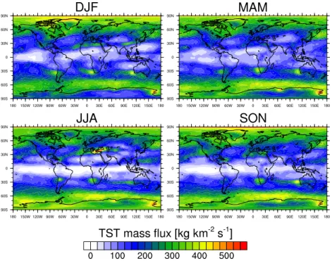
Fig. 3.Seasonally averaged TST mass flux for 1979–2011.
to 350 kg km−2s−1) in all seasons. STT along the storm
track over the Southern Ocean is quite uniform in SON and DJF and becomes more localized over Wilkes Land in East Antarctica during MAM and JJA (up to 450 kg km−2s−1). This is also when the most deep tropopause folds are found in this region (Sprenger et al., 2003).
3.1.2 Total TST mass flux
The annually averaged TST mass flux (Fig. 3) mainly shows large values poleward of approximately 55◦latitude in both
hemispheres and preferentially over the oceans and coastal regions. Distinct peaks are found along the north coast of Greenland (up to 475 kg km−2s−1 in DJF and around 400 kg km−2s−1in MAM and SON) and along the coast of Antarctica, especially over Mac. Robertson land near 70◦E
(reaching 500 kg km−2s−1 in MAM) and the
Transantarc-tic Mountains around 165◦E (peaking at 550 kg km−2s−1
in MAM, around 475 kg km−2s−1in other seasons). As
dis-cussed above, the deep tropopause folding activity is high in these regions in JJA, but since it is very low in DJF, this can-not be the only explanation for the quasi-permanent peaks observed.
In the subtropics, notable peaks are found over the east-ern Mediterranean and Anatolia (up to 525 kg km−2s−1 in JJA), the regions upstream of the continents around 30◦S
(all seasons), and over northern Africa (JJA, SON, DJF). Tropopause folds are quite frequent in all these regions and are especially deep over Anatolia (Sprenger et al., 2003). The importance of the western Pacific for tropical TST during
the Asian monsoon period is well known (e.g. Fueglistaler et al., 2004; Gettelman et al., 2004). Indeed, enhanced TST is visible on the eastern flank of the upper-level anticyclone in Fig. 3 in JJA and to a lesser extent also in SON.
3.1.3 STT mass flux through pressure surfaces
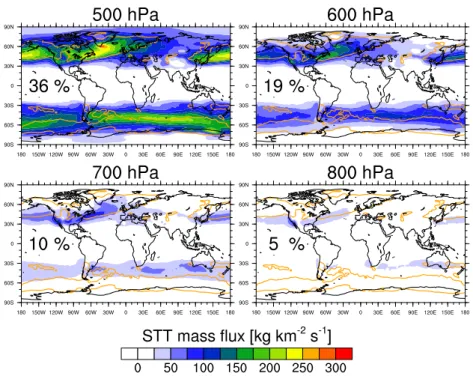
As mentioned in the Introduction, it is important to not only investigate the flux across the tropopause but also follow the STT air parcels as they descend into the troposphere. This is of course also true for TST air parcels in the stratosphere, but due to the focus of this study on quantifying the strato-spheric contribution to tropostrato-spheric ozone, we only discuss STT here. In Fig. 4, the mass flux across four pressure sur-faces is depicted and the areas with strongest fluxes across the tropopause are indicated with contours. For every tra-jectory, only the first crossing of a pressure surface is taken into account. One clearly visible feature is the equatorward transport of the air parcels as they descend. The peaks in the flux across the 700 hPa surface are on average located 10–15◦
closer to the Equator in the NH and approximately 20◦in the
SH than the peaks in the flux across the tropopause. This is readily explained by quasi-isentropic transport on isentropes sloping downwards towards the Equator due to the strong baroclinicity in the extratropics.
The flux across the 700 hPa surface is dominated by ex-changes in the North Atlantic and North Pacific storm tracks, a zonal band around 40◦S originating from exchanges along
Fig. 4.STT mass flux through the 500, 600, 700, and 800 hPa pressure surfaces of all STT events averaged over the period from 1979 to 2011 (annual mean). The orange contours indicate areas where the STT mass flux across the tropopause is greater than 300 kg km−2s−1.
The percentage values indicated in the panels are calculated with respect to the globally integrated STT mass flux across the tropopause.
also be seen from these plots is that only a small amount of exchange events are vertically deep and reach a pressure of 700 hPa or more (roughly 10 %). Also, for obvious reasons, there is no flux below 700 hPa in areas with high orography such as the Himalayas. This illustrates the need for a refined criterion for deep exchange events, compared to Wernli and Bourqui (2002), Sprenger and Wernli (2003) and James et al. (2003b), that is also applicable in mountain areas.
3.1.4 Mass flux from deep STT events into the PBL
The especially interesting cases where stratospheric air reaches the PBL within a few days (deep STT) are shown in Fig. 5. The flux into the PBL is depicted in colours and the contours indicate where the flux across the tropopause is largest. Note that these contours do not directly correspond to the flux shown in Fig. 2 because only the subset of deep exchanges is taken into account here.
Since the largest boundary layer heights in ERA-Interim are found over subtropical desert areas (Von Engeln and Teixeira, 2013), it is clear that dry regions with high orogra-phy in these latitudes facilitate the transport from the strato-sphere into the PBL and vice versa. Indeed, in both hemi-spheres, the subtropics around 30◦ and especially
moun-tain ranges near these latitudes are preferred regions of deep STT into the PBL. Very distinct maxima are found over the Rocky Mountains and the northern Sierra Madre (up to 220 kg km−2s−1 in MAM) as well as over the Himalayas
and the Tibetan Plateau (up to 250 kg km−2s−1in DJF and MAM).
The latter maximum is explained by the mechanism de-scribed above, which allows for a near-horizontal exchange of air between the stratosphere and the PBL. The high orog-raphy combined with intense heating leads to very high boundary layers, especially in the semiarid western part of the Tibetan Plateau and before the onset of the Asian mon-soon (Yanai and Li, 1994; Yang et al., 2004; Chen et al., 2013). The air masses transported to this region cross the tropopause over an area stretching from northern Africa to the Pamirs. The peak over the Rocky Mountains is of differ-ent nature since both the topography and the PBL height are lower, such that there more vertical transport is needed in or-der to reach the PBL. The air masses cross the tropopause at the end of the North Pacific storm track and slide down the isentropes in a southeastward direction. This roughly corre-sponds to the situation shown by Sprenger and Wernli (2003, their Fig. 6a).
The storm tracks in the North Atlantic and North Pacific are also areas of enhanced deep STT, which is especially in-teresting because of the relatively shallow marine PBL. The entrance into the PBL is shifted approximately 20◦
equator-ward from the crossing of the tropopause due to transport along sloping isentropes as discussed before. This implies that even areas south of 30◦N can be affected by
Fig. 5.Seasonally averaged deep STT mass flux into the PBL for 1979–2011. The orange contours indicate areas where the mass flux across the tropopause due to deep STT is higher than 25 kg km−2s−1.
MAM. We can confirm the finding of Sprenger and Wernli (2003) that a significant amount of air entering the PBL over and near the Mediterranean crosses the tropopause over the European Alps (their Fig. 6c). In MAM and JJA, there is also some deep STT reaching the PBL around the Hindu Kush, the Pamirs, the Altay Mountains, the Mongolian Plateau, and Gobi Desert. In the SH, most deep STT occurs in the subtrop-ics in JJA and SON with peaks over the Andes (between 20 and 30◦S), the Karroo in South Africa, and both over and
upstream of Australia.
Note that Fig. 5 is comparable with the “destinations” plot in Sprenger and Wernli (2003, their Fig. 5a). An obvious ex-ample of how the 700 hPa criterion (used in the above study) and the PBL criterion (used here) for deep exchanges differ is the fact that the peak over the Tibetan Plateau in DJF is only visible in our study.
3.1.5 Mass flux from deep TST events out of the PBL
The flux of air masses out of the PBL that will reach the stratosphere within 4 days (deep TST) is shown in Fig. 6. Clearly, the entrance of the North Atlantic and North Pacific storm tracks are preferred areas of deep TST in DJF (up to 125 kg km−2s−1) and to a lesser extent in MAM and SON. The air masses then cross the tropopause roughly 20◦
pole-ward, which agrees very well with the findings of Sprenger and Wernli (2003) in DJF (their Fig. 6d).
The Tibetan Plateau emerges as a distinct peak in DJF (350 kg km−2s−1) and especially in MAM
(450 kg km−2s−1). A closer look at the data reveals that these air masses mainly cross the tropopause over the northwestern Pacific (contour in Fig. 6), which corresponds to a fast upward and long-range eastward transport of approximately 6500 km in less than 4 days. In JJA, this eastward transport is slower and the air masses also cross the tropopause over eastern Siberia and the northwestern Pacific around 50◦N.
The Rocky Mountains and the adjacent areas to the east are regions with a strong deep TST flux out of the PBL during nearly the whole year with a maximum in MAM (175 kg km−2s−1) and a minimum in DJF. Additional anal-ysis reveals that most of this air crosses the tropopause over the Hudson Bay in JJA and SON, whereas this peak is shifted south over the Great Lakes area and the Canadian Shield in DJF and MAM (cf. contours in Fig. 6).
Fig. 6.Seasonally averaged deep TST mass flux out of the PBL for 1979–2011. The orange contours indicate areas where the mass flux across the tropopause due to deep TST is higher than 25 kg km−2s−1.
timescales used could also explain why the signal over north-ern Africa and the Arabian Peninsula visible in Berthet et al. (2007), where 30-day backward trajectories were calculated, is not present in our study.
In the SH, the flux out of the PBL occurs predominantly between 20 and 50◦S. In SON and DJF, mainly the
conti-nents are affected, especially the region east of the southern Andes (up to 110 kg km−2s−1) and the south coasts of Africa
and Australia. In MAM and JJA, areas of intense deep TST fluxes are also found along the storm track over the Southern Ocean.
3.2 Zonally integrated fluxes
The meridional profiles of the zonally integrated values of STT, TST, and net (STT-TST) mass fluxes are shown in Fig. 7. Also depicted are the fluxes due to deep exchange events across the tropopause (TP) and the top of the PBL. Overall, there is remarkably little interannual variability, in-dicating very robust patterns.
3.2.1 All exchanges
The STT mass flux features a broad peak in the extratropics in both hemispheres. The distribution in the NH is of trian-gular shape with a maximum around 45◦N, whereas the SH
exhibits a smeared-out double-peak structure caused by the superposition of two separate peaks near 30◦S (main peak,
due to the STJ) and near 60◦S (secondary peak, due to the
−100 −50 0 50 100
−90
−60
−30
0
30
60
90
STT TST
−8 −4 0 4 8
−90
−60
−30
0
30
60
90 Deep
STT Deep TST
TP
−8 −4 0 4 8
−90
−60
−30
0
30
60
90 Deep
STT Deep TST
PBL
Mass flux [105kg s−1km−1]
Latitude
Fig. 7. Meridional distribution of zonally integrated
STT NH a 12 %
J F M A M J J A S O N D
3.6
4.0
4.4
4.8
5.2
STT SH b 3%
J A S O N D J F M A M J
3.6 4.0 4.4 4.8 5.2 TST NH c 5%
J F M A M J J A S O N D
3.6
4.0
4.4
4.8
5.2 TST SH
d 9%
J A S O N D J F M A M J
3.6 4.0 4.4 4.8 5.2 Month
Mass flux [
10
10
kg s
−
1]
Fig. 8.Seasonal cycle of hemispherically integrated STT (blue, top)
and TST (red, bottom) mass fluxes by all exchange events in the NH (left) and SH (right) averaged from 1979 to 2011. The shading shows the 5th and 95th (light) and the 25th and 75th (dark) per-centiles of the monthly values, and the solid white line is the mean value of the 33 yr. The seasonality is quantified byS=maxmax−min
+min,
where max and min denote the maximum and minimum value of the mean cycle. Percentages ofSare shown in the individual plots.
storm track over the Southern Ocean, cf. Fig. 2). The sec-ondary peak in this superposition is clearly visible in the sea-sonal averages and especially in DJF, when the main peak is comparatively low (not shown).
The TST mass flux shows a complex structure consisting of two main peaks and one secondary peak in both hemi-spheres: one main peak is found around 55◦N and 60◦S due
to exchanges along the storm tracks (North Atlantic, North Pacific, Southern Ocean) and the other around 30◦N and
30◦S mainly due to exchanges near the STJ in the
Mediter-ranean (NH) and upstream of the continents (NH and SH) (cf. Fig. 3). In addition, there are two secondary tropical peaks around 10–15◦latitude in both hemispheres that are
better visible in the seasonal averages and are smeared out by the meridional displacement of the Intertropical Conver-gence Zone (not shown).
The net mass flux is directed downward between 30 and 70◦N and between 25 and 60◦S and upward in the tropics
between 25◦S and 25◦N, except for a narrow band with
near-zero net fluxes right at the Equator. Poleward of 70◦N and
60◦S, the net flux is very small and directed upward, which
agrees well with earlier studies (Juckes, 1997; Sprenger and Wernli, 2003, their Fig. 8).
3.2.2 Deep exchanges
Deep exchange trajectories cross the tropopause in the ex-tratropics and low polar regions in both directions (STT and TST) and hemispheres (NH and SH). The distributions for deep STT and deep TST indeed look very similar. The deep TST peak is shifted about 5◦to the north with respect to the
peak of deep STT in the NH, whereas in the SH the peaks are
Deep STT NH
a 83 %
J F M A M J J A S O N D
0
1
2
3 Deep STT SH
b 69 %
J A S O N D J F M A M J
0
1
2
3
Deep TST NH
c 33 %
J F M A M J J A S O N D
0
1
2
3 Deep TST SH
d 29 %
J A S O N D J F M A M J
0
1
2
3
Month
Mass flux [
10
9kg s
−
1]
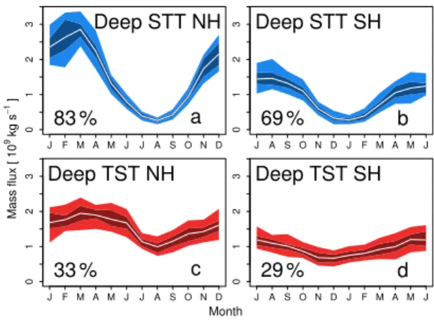
Fig. 9. Seasonal cycle of hemispherically integrated deep STT
(blue, top) and deep TST (red, bottom) mass fluxes in the NH (left) and SH (right) averaged from 1979 to 2011. The shading shows the 5th and 95th (light) and the 25th and 75th (dark) percentiles of the monthly values, and the solid white line is the mean value of the 33 yr. The seasonality is quantified and displayed as in Fig. 8.
very well aligned. The peaks in the SH are located around 60◦S, whereas the ones in the NH are located closer to the
Equator, around 50◦N. The peaks of the mass flux into (STT)
and out of (TST) the PBL are shifted, relative to the peaks of the TP crossings, towards the Equator by roughly 15◦in the
NH and 20–30◦in the SH. This shift is qualitatively in line
with the slope of the isentropes, which is particularly steep in the NH storm track regions. Note also that, in particular in the SH, the shift is larger for STT than TST, indicating that deep STT occurs on dry isentropes, whereas deep TST can be associated with saturated motion on moist isentropes from the PBL to the upper troposphere.
An interesting hemispheric difference is the greater inten-sity of deep STT and deep TST in the NH. The reason for this might be the more vigorous PBL dynamics over the more abundant NH continents.
3.3 Seasonal cycles
Monthly averages of STT and TST mass fluxes are calculated for the 33 yr covered in this climatology. As a simple mea-sure of the seasonality within a year, we consider the quotient
S=maxmax−+minmin, where max and min denote the maximum and
minimum averaged monthly values of the averaged annual cycle. This measure is essentially the ratio of the amplitude of the cycle and its mean value, such thatS=1 for a cycle
with a minimum value of zero.
3.3.1 All exchanges
around August and September. The minimum value is ap-proximately 22 % smaller than the peak value and the seasonality as defined above isS=12 %. In the SH (Fig. 8b),
the seasonal cycle is more sinusoidal in shape and much weaker (S=3 %) but its timing is roughly the same as in the
NH with a peak in winter (July) and a minimum in summer (December and January).
The seasonal cycle of the TST mass flux in the NH (Fig. 8c) also shows a rather sinusoidal cycle with a maxi-mum in November and a minimaxi-mum in May (S=5 %). In the
SH (Fig. 8d), a clear peak in March dominates the seasonal cycle. It is followed by a steep drop between April and June (due to fewer exchanges in the tropics) and a slow increase throughout the rest of the year (S=9 %).
Note that in contrast to the NH and SH cycles of STT, which peak in the same season, the NH and SH cycles of TST have quite different timing. In the NH, the maximum in TST is reached in late autumn, whereas in the SH, TST peaks in early autumn, corresponding to a shift of two months. The minima, on the other hand, occur nearly in the same month, namely in May (NH, late spring) and June (SH, early winter). In the NH, the STT and TST cycles are shifted by two to four months with TST occurring earlier in the year than STT. In the SH, the cycles of STT and TST are nearly re-versed with the minimum of TST being close to the max-imum of STT and vice versa. This asynchronous behaviour indicates that different meteorological phenomena contribute to the peaks in STT and TST.
The comparison of our seasonal cycles to previous stud-ies is not straightforward because some authors used either a different tropopause definition (Schoeberl, 2004) or inves-tigated only the extratropics (Sprenger and Wernli, 2003; James et al., 2003a), or even both (Olsen et al., 2004). Our results also do not fully agree with the classical study of Ap-penzeller et al. (1996), in which the net mass flux was found to have maxima in May (NH) and June (SH) and minima in September (NH) and October (SH). Our net mass flux (not shown) has broad maxima between January and March (NH) and June and August (SH) and minima in September (NH) and February (SH). The timing of our minimum in the NH and maximum in the SH thus agrees nicely with the men-tioned previous studies, and both our maximum in the NH and minimum in the SH are, although not being the main peaks, clearly visible in Appenzeller et al. (1996). When we restrict our analysis to the extratropics, as done in Sprenger and Wernli (2003) and James et al. (2003a), we obtain a sea-sonal cycle whose timing agrees quite well with their results (not shown).
3.3.2 Deep exchanges
The seasonal cycle of the mass flux due to deep STT events is shown in Fig. 9. The cycle for deep STT is much more pro-nounced than the one for all exchanges and shows a more si-nusoidal shape. The maxima occur in winter and early spring
260 280 300 320 340 360 380
0
10
20
30
STT
NH
DJF MAM JJA SON
260 280 300 320 340 360 380
0
10
20
30
STT
SH
260 280 300 320 340 360 380
0
10
20
30
TST
NH
260 280 300 320 340 360 380
0
10
20
30
TST
SH
Potential temperature [K]
A
ver
age mass flux [
10
7kg s
−
1K
−
1]
Fig. 10.Potential temperature distribution for STT (top) and TST
(bottom) in the NH (left) and SH (right) averaged from 1979 to 2011. The seasons are indicated by different line patterns as listed in the legend.
(March in the NH and August in the SH) and the minima in summer (August in the NH and January in the SH). The mini-mum in summer in the NH is less than 10 % of the maximini-mum value (S=83 %), whereas in the SH the minimum reaches
roughly 20 % of the peak value (S=69 %). Our seasonal
cy-cle of deep STT mass flux in the NH agrees very well with the results of Sprenger and Wernli (2003) and James et al. (2003b).
The deep TST mass flux shows a less regular seasonal cy-cle in the NH: the flux is relatively constant from January to June, followed by a sharp decrease with a minimum in Au-gust, after which it steadily increases until January. In the SH, the deep TST mass flux shows a broad maximum between March and July and a minimum in December. The minimum is roughly 55 % of the maximum value in both hemispheres, which shows that the seasonal cycle of deep TST (S=33 %
in the NH and 29 % in the SH) is much less pronounced than the one of deep STT. The deep TST mass flux in the NH is quite sinusoidal in Sprenger and Wernli (2003), whereas we observe a steep drop in early summer. This difference is due to the intense mass flux out of the PBL over the Tibetan Plateau in spring (not shown), which is not captured in the former study.
3.4 Potential temperature distributions
3.4.1 All exchanges
The distributions of2for all exchange events are depicted
in Fig. 10. Due to the seasonal cycle of the isentropes, ex-change in summer occurs on higher isentropes than in win-ter in both hemispheres and for both STT and TST. The2
260 280 300 320 340 360 380
0
1
2
3
Deep STT
NH
DJF MAM JJA SON
260 280 300 320 340 360 380
0
1
2
3
Deep STT
SH
260 280 300 320 340 360 380
0
1
2
3
Deep TST
NH
260 280 300 320 340 360 380
0
1
2
3
Deep TST
SH
Potential temperature [K]
A
ver
age mass flux [
10
7kg s
−
1K
−
1]
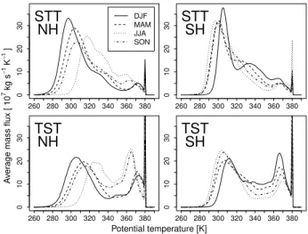
Fig. 11.Potential temperature distribution for deep STT (top) and
deep TST (bottom) in the NH (left) and SH (right) averaged from 1979 to 2011. The seasons are indicated by different line patterns as listed in the legend.
at2 >340 K than MAM. The reason for this is the intense
TST mass flux in the subtropics over the West Indies and the Caribbean in this season (not shown). There is a clear rela-tionship between2and the latitude at the exchange location.
In the tropics, exchanges occur at high potential temperatures above 350 K, and as the tropopause slopes down towards the polar regions, exchanges in the extratropics occur at lower potential temperatures, mainly between 280 and 350 K.
All distributions show a clear main peak below 350 K, varying from 295 K (STT NH DJF) to 325 K (TST NH JJA). Additionally, a smaller peak between 330 and 340 K is vis-ible for STT in the SH, especially in DJF, which is mainly due to exchanges over the Andes (see Fig. 2). The vast ma-jority of exchange events above 350 K occur in the tropics and subtropics between 25◦S and 30◦N (STT) and between
35◦S and 40◦N (TST) (not shown).
As expected, TST is larger than STT at high2, which
con-curs with a net upward transport in the tropics (cf. Fig. 7). Both for STT and TST, a prominent peak occurs at 380 K due to our tropopause definition. However, less than 1 % (STT) and 3 % (TST) of all exchanges take place at 380 K. As expected, this peak is much stronger for TST than for STT and its geographical distribution is limited to a narrow band between 10◦S and 10◦N (not shown).
As already discussed in Sprenger and Wernli (2003), stud-ies of STE that are limited to specific isentropes, such as 330 and 350 K (Seo and Bowman, 2001), capture only a fraction of all STE events and might produce a seasonal cycle that is not representative of total STE.
3.4.2 Deep exchanges
The2distributions for deep exchange events only are shown
in Fig. 11. All peaks are sharper and limited to the region
be-1980 1985 1990 1995 2000 2005 2010
80
90
100 STT −1.83e+06
p = 2.92e−01
1980 1985 1990 1995 2000 2005 2010
−5
0
5
10
STT−TST 7.46e+06 p = 2.02e−07
1980 1985 1990 1995 2000 2005 2010
80
90
100 TST −9.29e+06
p = 1.34e−07
1980 1985 1990 1995 2000 2005 2010
2
3
4
Deep STT 9.84e+05 p = 1.07e−03
1980 1985 1990 1995 2000 2005 2010
2
3
4
Deep TST 3.98e+05 p = 4.33e−02
Mass flux [
10
9kg s
−
1 ]
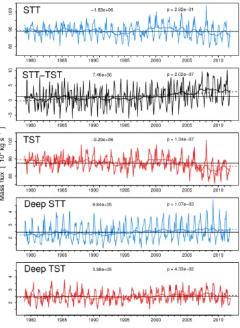
Fig. 12.Time series of globally integrated STT, net (STT–TST),
TST, deep STT, and deep TST mass fluxes (monthly averages) from 1979 to 2011. The bold line is a 12-month moving average, the thin horizontal line (solid) is the mean value of the 33 yr, and the thin sloping line (dashed) is the fit from a linear regression over the whole period. The trends (top middle) in kg s−1month−1andp
val-ues (top right) are shown within the individual figures.
low 350 K, which is mainly due to the fact that very few deep exchange events occur in the tropics (cf. Fig. 7). A notable exception of the otherwise dominating single-peak structure is the deep STT distribution in the NH in JJA, which features a second, smaller peak around 330 K due to exchanges over the eastern Mediterranean and Anatolia (not shown). Again, the summer peaks are found at higher 2 than the winter
peaks. The seasonal variation of the most likely2is larger
in the NH (20–25 K) than in the SH (10–15 K).
3.5 Time series
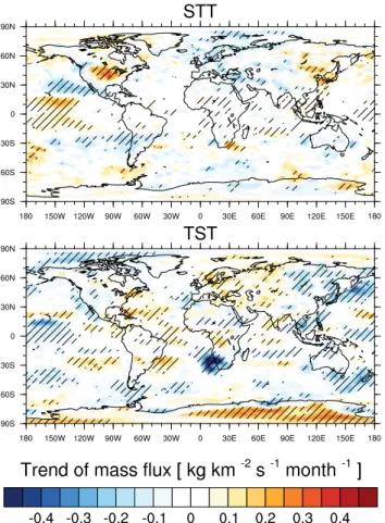
Fig. 13.Trends of STT (top) and TST (bottom) mass flux from 1979 to 2011. Linear regression is applied to monthly averages at every grid point, and regions where the trends are significant on a 1 % level are dashed. The trend west of South Africa is approximately
−0.75 kg km−2s−1month−1.
and Wernli (2003) for the ERA-15 period); thereafter both fluxes decline. The upward flux declines more strongly than the downward flux, resulting in a small increase in the net downward flux after 2000. Linear regression analysis for the whole time series yields highly significant (pvalue∼10−7)
trends for TST (−9.29×10⁶kg s−1month−1) and STT-TST
(7.46×10⁶kg s−1month−1).
Since our study covers the whole globe, the non-zero global net downward mass flux has two possible interptations: either the real net mass flux is zero and our re-sult is due to numerical and methodological errors or the mass of the troposphere is increasing. The latter case would go along with a rise in tropopause heights which was re-ported in previous studies (e.g. Steinbrecht et al., 1998; Sei-del and RanSei-del, 2006; Schmidt et al., 2008). To further analyse this, we have calculated the area-weighted average pressure at the tropopause and the mass of the troposphere for every 6-hourly time step of ERA-Interim from 1979 to 2011. Linear regression analysis reveals highly signifi-cant (p <2×10⁻¹⁶) trends of−0.050±0.016 hPa yr−1and
2.843±0.083×10¹⁴kg yr−1, in agreement with the studies
mentioned above. This calculation thus suggests that the non-zero net downward mass flux is not a numerical artefact.
In addition to the trends of globally integrated mass fluxes, we have also analysed local trends. To this end, at every grid point (1◦×1◦), time series of monthly averaged mass
fluxes from 1979 to 2011 are used to perform a linear re-gression. As can be seen from Fig. 13, there are large dif-ferences between regions. While the STT mass flux shows no significant trend globally (see above and Fig. 12), sig-nificant (p <0.01, dashed areas in Fig. 13) and
compara-tively strong trends are found in many regions. The most intense positive trend is observed over central North Amer-ica (0.38 kg km−2s−1month−1, accompanied by a zonally
aligned dipole structure over the North Pacific of magnitude
±0.25 kg km−2s−1month−1), indicative of an equatorward
shift. Negative trends are most notably found over Anatolia, the southwestern tip of Scandinavia, and the Andes around 30◦S (approximately−0.30 kg km−2s−1month−1).
The geographical distribution of trends in TST mass flux (bottom plot in Fig. 13) shows significant and strong positive trends over Antarctica, especially on its east-ern side (up to 0.32 kg km−2s−1month−1), even stronger negative trends over the northwestern Pacific (up to
−0.41 kg km−2s−1month−1), and southwest of southern
Africa (up to−0.76 kg km−2s−1month−1). The dipole
struc-ture over the North Pacific is again visible but the sign is re-versed when compared to the STT mass flux trend. These zonally aligned dipole structures can also be found over the South Pacific and the Indian oceans, indicating a systematic poleward shift of the TST mass flux in the subtropics. The reason for these patterns is not clear and thus requires more detailed future investigation.
Both the globally integrated deep STT and deep TST mass fluxes increase over time (see Fig. 12). The trend ob-tained from linear regression analysis for the whole time series is more than twice as strong and much more signifi-cant for the deep STT mass flux (9.84×10⁵kg s−1month−1, p≈0.001) than for the deep TST mass flux (3.98×
105kg s−1month−1, p≈0.04). These trends are heavily influenced by positive trends over central and western North America (see Fig. S1 in the Supplement), with magnitudes of approximately 0.13 kg km−2s−1month−1and
0.17 kg km−2s−1month−1 for deep STT and deep TST,
re-spectively.
4 Ozone flux into the troposphere
Fig. 14.Seasonally averaged ozone mixing ratios per volume (ppbv) at the 2 pvu/380 K dynamical tropopause for 1979–2011.
ozone concentrations at the tropopause in boreal spring and summer over the eastern US, the North Atlantic, the Mid-dle East, and large parts of central Asia. In this section, due to the importance of investigating the stratospheric influence on near-surface ozone concentrations, we focus on the STT ozone flux. A brief discussion of the TST ozone flux can be found in Sect. 6.3.
The globally integrated STT ozone flux calculated in our study amounts to 420 Tg yr−1, which is within the estimates
from models (556±154 Tg yr−1; Stevenson et al., 2006) and
observations (550±140 Tg yr−1; Solomon et al., 2007). All
calculations with the ozone field of ERA-Interim of course crucially depend on its quality. Dragani (2011) found that overall the ozone field agrees well with independent obser-vations and performs better than in the earlier ERA-40 re-analysis. The relative errors in total column ozone are within
±2 % between 50◦S and 50◦N, but the vertical profiles show
errors of up to 20 % in the lower stratosphere. Therefore, our results have to be interpreted with these limitations in mind.
4.1 Geographical distribution
The geographical distribution of the STT ozone flux through the tropopause is shown in Fig. 16. Areas of intense STT
mass flux such as the storm tracks in the North Atlantic, the North Pacific, and the Southern Ocean also tend to show elevated values of the STT ozone flux. Nevertheless, there are some differences when comparing the mass flux (Fig. 2) with the ozone flux (Fig. 16) that originate from the strong seasonal and geographical variation of ozone at the tropopause (Fig. 14). In DJF, the ozone concentrations over the NH storm tracks are rather small, such that the domi-nant peak in ozone flux is located over the Andes in the SH (nearly 240 kg km−2month−1), where tropopause ozone
con-centrations are nearly twice as high. The peak over south-ern Greenland in the mass flux in MAM and SON is less prominent in the ozone flux due to the low ozone concen-trations in this region. In JJA, the same areas show high mass and ozone fluxes (e.g. central North America, Anato-lia, Pamirs, Tian Shan, northern China, Korea), with peaks up to 300 kg km−2month−1. The JJA ozone flux is dominant in the NH, whereas the mass flux is more balanced between the hemispheres, a consequence of the strong hemispheric contrast in ozone concentration at the tropopause. An addi-tional peak in the STT ozone flux is found along the Equator over the Indian Ocean (nearly 220 kg km−2month−1) due to
Fig. 15.Zonal and annual average of ozone mixing ratio and dif-ferent tropopause definitions in ERA-Interim for 1979–2011. The blue, red, and white lines show the lapse-rate tropopause as de-fined by the WMO (“LRT”), the 3.5 pvu/380 K control surface (“3.5 pvu”) and the 2 pvu/380 K dynamical tropopause (“2.0 pvu”), respectively. Note the non-linear colour scale.
The global peaks of the STT ozone flux are thus found over the Andes around 35◦S in DJF, over the Himalayas
and the southern side of the Tibetan Plateau in MAM (up to 260 kg km−2month−1), and over central North America,
Anatolia, the Pamirs, Tian Shan as well as large parts of eastern Asia in JJA (also up to 290 kg km−2month−1). These
findings are consistent with the studies of Hsu et al. (2005) and Tang et al. (2011).
The geographical distribution of the deep STT ozone flux into the PBL shown in Fig. 17 indicates the re-gions where surface ozone levels are most likely af-fected by stratospheric intrusions. Western North Amer-ica (in MAM) and the Tibetan Plateau (in DJF, MAM, and JJA) are the global hotspots with peaks values of more than 120 kg km−2month−1. For the calculation of this flux, the ozone concentration was kept constant within the troposphere (that is, any loss due to chemical processes and mixing was neglected) and therefore these values provide an upper boundary estimate. Nevertheless, our findings are in agreement with observational studies in these areas, which find a significant stratospheric influence (e.g. Langford et al., 2009; Cristofanelli et al., 2010; Lefohn et al., 2011, 2012; Lin et al., 2012).
4.2 Seasonal cycle
The seasonal cycle of the STT ozone flux (top row in Fig. 18), withS=25 % in the NH and S=13 % in the SH, shows
a very different pattern than the STT mass flux (top row in Fig. 8). Indeed, maxima of the ozone flux occur when the mass flux is nearly at its minimum and vice versa. The ex-planation for this result is that the ozone concentration at the tropopause during STT events (bottom row in Fig. 18) shows a nearly sinusoidal seasonal cycle with a maximum in sum-mer (around 130 ppbv in the NH and 105 ppbv in the SH) and a minimum in winter (around 75 ppbv in the NH and 80 ppbv in the SH). Even though the mass flux in summer is about 20 % smaller than in winter, the ozone concentration is around 65 % larger and thus overcompensates for the reduc-tion in mass flux. This can also be quantified in terms of the seasonalityS: for the STT mass flux,S=12 % in the NH and S=3 % in the SH (cf. Sect. 3.3), whereas the ozone
concen-trations at the tropopause have a larger seasonality, namely
S=25 % in the NH andS=13 % in the SH.
In contrast to the total ozone flux, the ozone flux for deep exchange events only (middle row in Fig. 18) largely agrees in its timing with the mass flux (top row in Fig. 9). This is because the seasonality of the mass flux is large enough to dominate the ozone flux: its value in summer is reduced by approximately 90 % compared to winter (S=83 % in the
NH andS=69 % in the SH, cf. Sect. 3.3). The peak in the
deep STT ozone flux is slightly shifted (one month later com-pared to the mass flux) in both hemispheres. This is due to the increase of ozone concentrations at the tropopause dur-ing sprdur-ing (cf. bottom row in Fig. 18). A remarkable conse-quence is that while the seasonal cycle of deep STT is simi-lar to the whole STT mass flux, this is not true for the ozone flux. In fact, the deep STT ozone flux is shifted by roughly 4 months with respect to the STT ozone flux and peaks in early spring.
4.3 Time series
The global STT ozone flux shown in Fig. 19 slightly in-creases from 1979 to late 1991. It then is reduced during 3 yr and increased notably between 1994 and late 2001. Between early 2002 and mid-2003, there is a striking jump and the ozone flux is roughly halved. Afterwards, it recovers again in 2004, stays nearly constant for 4 yr, and begins to decrease slightly after 2009. Details on these spurious jumps and pos-sible explanations are discussed in Sect. 6.3.
5 Sensitivity studies
Fig. 16.Seasonally averaged STT ozone flux for 1979–2011.
Fig. 17.Seasonally averaged deep STT ozone flux into the PBL for 1979–2011. For this calculation, the ozone concentration is kept constant
STT NH a
25%
J F M A M J J A S O N D
10
14
18
22
26 STT SH b
13%
J A S O N D J F M A M J
10
14
18
22
26
Deep STT NH c
75%
J F M A M J J A S O N D
0
0.2
0.4
0.6
0.8
1
1.2
1.4
Deep STT SH d
63%
J A S O N D J F M A M J
0
0.2
0.4
0.6
0.8
1
1.2
1.4
J F M A M J J A S O N D
50
70
90
110
130
150
NH e
25%
J A S O N D J F M A M J
50
70
90
110
130
150
SH f
14%
Month
Oz
one at TP [ ppb
v ] Oz
one flux [ Tg month
−
1]
Fig. 18.Seasonal cycles of hemispherically integrated STT ozone
flux (top) and deep STT ozone flux (middle) in the NH (left) and SH (right) averaged from 1979 to 2011. The bottom row shows the ozone mixing ratios at the 2 pvu/380 K dynamical tropopause. The shaded areas show 5th and 95th (light) as well as 25th and 75th (dark) quantiles of the monthly values. The solid white lines show the mean values of the 33 yr. The seasonality is quantified by
S=maxmax−min
+min, where max and min denote the maximum and
min-imum value of the mean cycle. Percentages ofSare shown in the
individual plots.
sensitivity, we calculated STE fluxes for the year 2010 using various combinations of the parameters mentioned above. Despite the noisiness of the results (due to the consideration of only one year), systematic effects are clearly visible.
5.1 Choice of control surface
STE fluxes critically depend on the choice of the control sur-face. To emphasize the quasi-material character of the dy-namical tropopause, we use a fixed value of PV and note that the choice of the “best” PV value representing the trans-port barrier between the troposphere and the stratosphere is non-trivial and varies between different isentropes and sea-sons (Kunz et al., 2011). In our opinion, among all the pos-sible control surfaces used to indicate the position of the tropopause, there exists no definition which is superior in all aspects and situations. The choice of a constant PV sur-face as the dynamical tropopause is meaningful and, when combined with the analysis of additional PV surfaces, allows for the three-dimensional structure of STE to be understood. Bourqui (2006) studied transport across PV surfaces ranging from 1 to 5 pvu but in this section, we focus on the “classical” values of 2.0 and 3.5 pvu. The “3.5 pvu” STE data set is thus
1980 1985 1990 1995 2000 2005 2010
15
20
25
30
35
40
45
50
Oz
one flux [ Tg month
−
1]
STT Ozone
Fig. 19. Time series of the globally integrated STT ozone flux
(monthly averages) from 1979 to 2011. The bold line shows a 12-month moving average and the mean value of the whole time series is indicated with a horizontal line.
obtained by choosing the combination of the ±3.5 pvu PV
isosurfaces and the 380 K isentrope as the control surface. In the zonal average, this choice corresponds well to the lapse-rate tropopause as defined by the World Meteorological Or-ganization (WMO, 1957; Hoinka, 1998). While this is also true for the temporally and zonally averaged ERA-Interim data set used in this study (see Fig. 15), the degree of agree-ment varies strongly for different synoptic flow systems.
● ● ● ● ● ● ● ● ● ● ● ●
STT NH a
J F M A M J J A S O N D
0.8
0.9
1
max control = 4.63 max highres = 4.69 max 3.5 pvu = 2.81 ● control highres 3.5 pvu ● ● ● ● ● ● ● ● ● ● ● ●
STT SH b
J A S O N D J F M A M J
0.8
0.9
1
max control = 4.75 max highres = 4.76 max 3.5 pvu = 3.03
● ● ● ● ● ● ● ● ● ● ● ● STT NH c
max control = 21.83 max highres = 22.2 max 3.5 pvu = 19.37
J F M A M J J A S O N D
0.4 0.5 0.6 0.7 0.8 0.9 1 ● ● ● ● ● ● ● ● ● ● ● ● STT SH d
max control = 15.85 max highres = 15.9 max 3.5 pvu = 13.74
J A S O N D J F M A M J
0.4 0.5 0.6 0.7 0.8 0.9 1 ● ● ● ● ● ● ● ● ● ● ● ● max control = 118.08
max highres = 118.08 max 3.5 pvu = 162.38
J F M A M J J A S O N D
40 60 80 100 120 140
160 NH e
● ● ● ● ● ● ● ● ● ● ● ● max control = 85.39
max highres = 85.39 max 3.5 pvu = 126.01
J A S O N D J F M A M J
40 60 80 100 120 140
160 SH f
Month
Oz
one at TP [ ppb
v ] Oz
one flux [ Tg month
−
1] Mass flux [ 10
10
kg s
−
1 ]
Fig. 20.Seasonal cycles of hemispherically integrated STT fluxes
of mass (top) and ozone (middle) for the year 2010. The three dif-ferent data sets (“control”, “highres”, and “3.5 pvu”) are described in Sect. 5. In the bottom row, the average mixing ratio of ozone at the corresponding control surface is shown. The seasonal cycles are scaled to their maximum values shown within the individual figures, facilitating the comparison of amplitude and shape of the cycles.
effect of the higher ozone concentrations, leading to a re-duction of more than 60 % of the deep STT ozone flux (see Fig. S2 in the Supplement). The shapes of the seasonal cycles are very similar in both data sets. For TST, the situation is similar (see Fig. S3): the mass flux across the 3.5 pvu surface is reduced by approximately 34 % in both hemispheres. The deep TST mass flux is strongly reduced by approximately 70 %. Although STT and TST are slightly differently affected by the change in control surface, the shape of the seasonal cycle of the net (STT-TST) mass flux is very similar in both data sets (see top row in Fig. S4) and the maximum values are reduced by 43 % (NH) and 27 % (SH).
We have further compared the geographical patterns of the STE mass fluxes by scaling the fluxes in both data sets to their respective global maximum (see Figs. S5–S8). Sim-ilarly to the hemispherically integrated values mentioned above, the global maxima of STT and TST mass fluxes are reduced by 27 and 44 %, respectively. Patterns of the STT mass flux are very similar for the two control surfaces, while for the TST mass flux, the relative importance of the tropics is strongly increased in the 3.5 pvu data set. This is due to the combination of identical STE fluxes across the 380 K isen-trope in both data sets and an overall reduction of the STE
● ● ● ● ● ● ● ● ● ● ● ● ● ● ● ● ● ● ● ● ● ● ● ● ● ● ● ● ● ● ● ● ● ● ● TP
κ = −0.76
400 hPa −0.58 500 hPa −0.5 600 hPa −0.48 700 hPa −0.48 800 hPa −0.49 PBL −0.5
48 60 72 84 96
0.25 0.5 1 2 3 4 5 7 9
Minimum residence time τ [h]
T
otal STT mass flux [
10
19
kg ]
Fig. 21.Globally integrated STT mass flux across the tropopause,
pressure surfaces from 400 to 800 hPa, and into the PBL aver-aged for 1979–2011. Note the double-logarithmic scale. The flux decreases with increasing minimum residence time thresholdτ as
a power law (that is, the flux is proportional toτκ). The fitted
ex-ponentsκ(R2>0.995 for all fits) are listed adjacent to the corre-sponding curves.
flux across the higher PV isosurface. The fact that this effect is not visible for STT suggests that even in the tropics, STT occurs predominantly across the PV isosurface and not the 380 K isentrope, in agreement with the potential temperature distribution shown in Fig. 10.
The net upward transport in the polar regions across the 2 pvu tropopause (see Fig.7) is strongly reduced in the 3.5 pvu data set, mainly due to a relative decrease in TST compared to STT (see Fig. S9). This result is not in con-flict with the large-scale subsidence in polar regions related to the Brewer–Dobson circulation, because the latter applies to pressure levels around 100 hPa (Holton et al., 1995), while both PV isosurfaces used in this study are typically situated far below (between 275 and 350 hPa; see Fig. 15). Therefore, the reduced upward net flux in the 3.5 pvu data set indicates that the majority of TST events in polar regions are vertically shallow.
While the hemispherically integrated deep STE fluxes are reduced by more than 68 % (see above), the global maxima are only reduced by 59 and 45 % for deep STT and deep TST, respectively. The regions with strong deep STE flux across both the 2 pvu and the 3.5 pvu isosurfaces are predominantly
located in the extratropics (not shown) and the location of the “hot spots” of deep STE flux across the PBL top is not affected by the different control surfaces used.
5.2 Trajectory spacing
dp=15 hPa in the extratropics, and dp=5 hPa in the
trop-ics). As a consequence, the number of trajectories calcu-lated is increased by a factor of 8. The seasonal cycles are only very slightly affected by this increase in resolution (see Figs. 20, S2, and S3) and the geographical patterns are also robust (not shown). Thus the trajectory starting grid used in our study (see Sect. 2) is already sufficiently dense.
5.3 Minimum residence time
The quantitative results for all fluxes in this study strongly depend on the choice of the minimum residence time τ
(Bourqui, 2001; Wernli and Bourqui, 2002; Bourqui, 2006). This is a fundamental property of any advective–diffusive flow across a control surface such as the tropopause (Hall and Holzer, 2003; Orbe et al., 2012). Clearly, the flux across a chosen surface decreases with increasingτand vanishes for τ→ ∞. In the limitτ →0 the flux diverges due to
molecu-lar diffusion (Hall and Holzer, 2003).
We have studied the globally integrated fluxes of mass and ozone across the tropopause, pressure surfaces between 400 and 800 hPa, and the PBL top forτ between 48 and 96 h.
The results depicted in Fig. 21 show that the dependency onτ is, to very good approximation, a power law, i.e.
pro-portional to τκ. The fitted exponents κ for the mass flux
across the pressure surfaces below 500 hPa and into the PBL are very close to−0.5 (−0.49±0.01), and for the 400 hPa
surface and the tropopause the values are−0.58±0.01 and −0.76±0.02, respectively. For the STT ozone, TST mass
and TST ozone fluxes, the fitted exponents are of similar magnitude and can be found in Table 1 of the Supplement. The power law applies with remarkable precision: all coef-ficients of determination,R2, are greater than 0.995. These
results are in agreement with theory, which suggests that for any advective–diffusive flow, the (mass) flux across a control surface such as the tropopause is proportional toτ−0.5 for
smallτ in the continuum limit (Hall and Holzer, 2003; Orbe
et al., 2012). Note though that theτ used in these studies is
only a one-sided criterion – that is, it is only required that the air parcels stay for at leastτ in the stratosphere (in the case
of STT) – whereas our minimal residence timeτ is a
two-sided criterion (before and after the exchange). The findings of Bourqui (2006) and Wernli and Bourqui (2002) support the assumption that this power law fit can be extended to the range ofτ between 12 and 48 h. Thus our calculated STE
flux, at least for the lower pressure surfaces and the PBL, is clearly in the diffusive regime described in Hall and Holzer (2003) for a large range ofτ up to 96 h.
While the amplitude of STE fluxes of mass and ozone are highly sensitive to this parameter, this is not true for the geographical patterns (now shown), such that our choice of
τ=48 h (see Sect. 2), well above the lower limit of 8 h
sug-gested by Bourqui (2006), does not limit the generality of the conclusions reached in this manuscript.
6 Discussion
In this section, we want to address caveats of the method, compare our results to previous studies and discuss our re-sults in selected regions.
6.1 Caveats of the method
Caveats of our method are related, for instance, to the quality of the PBL height parameter and the ozone field in the ERA-Interim data, as well as to the poor representation of sub-grid-scale processes.
Our methodology to quantify deep STE relies strongly on the quality of the diagnosed PBL height in the ECMWF model. The method used in the ERA-Interim forecasts, following Troen and Mahrt (1986), is based on the bulk Richardson number and is suitable for global model output. Seidel et al. (2012) reported that the PBL height in ERA-Interim is likely up to several 100 m too high, especially over high-elevation regions. We have investigated this influence by limiting the pressure at the PBL top to a minimum of 330 hPa, which roughly corresponds to the PBL height mea-sured over the Tibetan Plateau in Yang et al. (2004). This limitation only affects the amplitudes of the deep STE fluxes in this region (a reduction of∼25 % in DJF and∼35 % in
MAM), but the influence on the hemispherically integrated seasonal cycles is negligible (not shown). The importance of the Tibetan Plateau for deep STE is thus not fundamentally questioned by this investigation, but a considerable amount of deep STE in this region occurs when the PBL top reaches very high altitudes, and thus a possible bias of a few hun-dred metres can have a large impact on the exact values of the peak. Considering the recent measurements of very high boundary layers over the Tibetan Plateau (Chen et al., 2013), we chose not to restrict the PBL height in our study.