Molecular Structure Dynamics by Cryo-Electron
Tomography of a Single-Molecule Structure
Lei Zhang, Gang Ren*
Molecular Foundry, Lawrence Berkeley National Laboratory, Berkeley, California, United States of America
Abstract
The dynamic personalities and structural heterogeneity of proteins are essential for proper functioning. Structural determination of dynamic/heterogeneous proteins is limited by conventional approaches of X-ray and electron microscopy (EM) of single-particle reconstruction that require an average from thousands to millions different molecules. Cryo-electron tomography (cryoET) is an approach to determine three-dimensional (3D) reconstruction of a single and unique biological object such as bacteria and cells, by imaging the object from a series of tilting angles. However, cconventional reconstruction methods use large-size whole-micrographs that are limited by reconstruction resolution (lower than 20 A˚), especially for small and low-symmetric molecule (,400 kDa). In this study, we demonstrated the adverse effects from image distortion and the measuring tilt-errors (including tilt-axis and tilt-angle errors) both play a major role in limiting the reconstruction resolution. Therefore, we developed a ‘‘focused electron tomography reconstruction’’ (FETR) algorithm to improve the resolution by decreasing the reconstructing image size so that it contains only a single-instance protein. FETR can tolerate certain levels of image-distortion and measuring tilt-errors, and can also precisely determine the translational parameters via an iterative refinement process that contains a series of automatically generated dynamic filters and masks. To describe this method, a set of simulated cryoET images was employed; to validate this approach, the real experimental images from negative-staining and cryoET were used. Since this approach can obtain the structure of a single-instance molecule/particle, we named it individual-particle electron tomography (IPET) as a new robust strategy/approach that does not require a pre-given initial model, class averaging of multiple molecules or an extended ordered lattice, but can tolerate small tilt-errors for high-resolution single ‘‘snapshot’’ molecule structure determination. Thus, FETR/IPET provides a completely new opportunity for a single-molecule structure determination, and could be used to study the dynamic character and equilibrium fluctuation of macromolecules.
Citation:Zhang L, Ren G (2012) IPET and FETR: Experimental Approach for Studying Molecular Structure Dynamics by Cryo-Electron Tomography of a Single-Molecule Structure. PLoS ONE 7(1): e30249. doi:10.1371/journal.pone.0030249
Editor:Wenqing Xu, University of Washington, United States of America
ReceivedJuly 6, 2011;AcceptedDecember 14, 2011;PublishedJanuary 24, 2012
This is an open-access article, free of all copyright, and may be freely reproduced, distributed, transmitted, modified, built upon, or otherwise used by anyone for any lawful purpose. The work is made available under the Creative Commons CC0 public domain dedication.
Funding:This work was supported by the Office of Science, Office of Basic Energy Sciences of the United States Department of Energy (contract no. DE-AC02-05CH11231) and partially supported by the William Myron Keck Foundation (#011808). The funders had no role in study design, data collection and analysis, decision to publish, or preparation of the manuscript.
Competing Interests:The authors have declared that no competing interests exist.
* E-mail: [email protected]
Introduction
The dynamic character of proteins dictates their functions and ultimately represents an accurate portrayal of their many ‘‘personalities’’ [1,2]. A snapshot of proteins frozen in crystals reveals a single, unique structure that is often used as a blueprint for studies in structure–function relationships. However, these structures fail to encompass the dynamic nature of proteins in solution. Protein dynamics involves both equilibrium fluctuations that regulate biological function and other non-equilibrium effects of biological motors, which convert chemical energy to mechanical energy.
Although the experimental approach to determine the dynamic structure at atomic-resolution level is not available, molecular dynamics (MD) simulations have been widely used to link structure and dynamics by enabling the exploration of the conformational energy landscape accessible to protein molecules [1,2]. MD simulations could provide detailed dynamics and function in structure, but one of the major obstacles of MD is a potential
energy barrier to determine global protein conformations and equilibrium fluctuations.
and the high-density lipoprotein (HDL), the classification and orientation determination of subvolumes are challenging. More-over, the average of hundreds of different conformational structures could be detrimental to elucidate the structural equilibrium fluctuations of a protein.
We believe, there are adverse effects from image distortion and measuring tilt-errors in conventional tomography reconstruction methods, which play a major role in limiting the resolution of the large-size whole micrograph reconstruction. The image distortions (introduced by lens astigmatism [8], energy filter [9,10], radiation-induced deformations [11] and defocus-related distortion) can generate the displacement (translational errors) and measuring tilt-errors (including tilt-axis and tilt-angle tilt-errors). Since measuring tilt-angle is usually performed by tracking the movements of gold fiducial markers between the tilt micrographs, the inconsistency of displacement introduced by image distortion results in the inconsistency of movement of markers during tilting, therefore resulting in an inconsistency of tilt-angles. The final determined tilt-angle is actually an average of tilt-angles suggested from different areas of the micrograph. Greater distortion results in greater displacement, thus producing a larger tilt-angle error. Image distortion is generally a large-scale deformation/displace-ment, in which different areas within a micrograph present a different amount of displacement. Mathematically, large-scale deformation/distortion can be represented by a combination of local displacement (translational error), rotation (tilt-axis error) and tilting (tilt-angle error). For example, in two-dimensional (2D) cryo-crystallography, the uneven supporting substrate can fre-quently introduce a large-scale distortion of 2D crystal. The distortion introduces a displacement and rotation against space. The distortion can be determined and corrected by a so-called ‘‘unbending’’ image-processing method [12,13]. In brief, the whole micrograph image is broken into a series of small-size images to calculate the translation/displacement and rotation of each small image via a comparison of each small image to the average image/reference. Shifting and rotating back each small image according to its determined displacement and rotational parameters can correct the distortion of large-size crystal/ micrograph by merging these shifted/rotated small-images together. However, in cryoET reconstruction, either the lattice or the averaged reference is not available to correct the distortion of the large-size micrograph. The measuring tilt-errors (including the displacement-introduced tilt-error and the distortion-intro-duced small rotation and tilting) can limit the resolution of the large-size whole micrograph reconstruction. A simple model to estimate the tilt-errors is to treat them as a random vibration within a small range, such as60.5u. This requires a new strategy that can tolerate these tilt-errors and can precisely determine/ correct the translational errors/displacement for high-resolution cryoET reconstruction.
Here, we report a new strategy and robust algorithm, focused ET reconstruction (FETR) that can tolerate small tilt-errors and accurately determine two translational parameters of each image. FETR is an iterative refinement procedure that includes a series of automatically generated dynamic filters and masks for enhancing the convergence of the reconstruction. To limit the adverse effects from the tilt-errors, we reduced the size of reconstruction ET images by containing only a single-instance of a protein particle, rather than large whole-micrograph images that contain dozens of proteins from conventional methods. Hence, we named this approach individual-particle electron tomography (IPET) [14]. We believe that, with the same uncorrectable tilt-errors, the maximum translational error (displacement) within a small image is much smaller than within a large whole-micrograph. The small
image-size can limit the translational error from measuring tilt-errors, which can further limit the adverse effects from tilt-errors in the 3D reconstruction.
To describe the IPET method and FETR algorithm, a set of simulated cryoET images were generated and used. To validate this reconstruction method, four sets of real experimental ET data consisting of two sets of an antibody (molecular weight:
,150 kDa) imaged by negative-staining ET, and two sets of
nascent HDL (molecular weight: 140–240 kDa, protein portion: 56–84 kDa) imaged by cryoET [15] were used for 3D reconstruc-tion of each targeted single-instance protein. All four 3D reconstructions displayed abundant structural details, such as the domains. The most interesting feature of this method is that the 3D reconstruction of each individually targeted molecule instance is free of conformational dynamics and heterogeneity, proving that the 3D structure can be treated as a snapshot of the dynamic structure of the macromolecule. By comparing these ‘‘snapshot’’ structures, this method could allow the study of macromolecular structural dynamics [16,17,18]. The global protein conformations and equilibrium fluctuations can be used as a constraint for MD simulation to reveal the structural detail in protein function and mechanism.
Methods
1 Generating simulated cryoET data
Build-up of a targeted object: To introduce the IPET method and FETR algorithm, a set of simulated cryoET data was generated from a known-answer object. The targeted object is a single instance of protein, a fragment (A–D chains, molecular weight: ,108 kDa) of molybdate transporter (ModB2C2) from Archaeoglobus fulgidus(PDB entry 2ONK [19]). The 3D density map of the object was generated at a resolution of 2 A˚ within a box of 16061606160 voxels by the ‘‘pdb2mrc’’ command (EMAN software package) [20], in which each pixel corresponds to 1 A˚ in the specimen (a magnification of ,100 kX when using a
4 k64 k CCD camera). The feature of using this targeted object is that it contains various structural features that can be used to evaluate the reconstruction at various resolutions, such as a donut-like overall shape (,100 A˚ in longest diameter), central hole (a
diameter of,30 A˚ ), 12 transmembrane a-helix domains (,10–
20 A˚ ), and shorta-helices andb-strands (,8 A˚ and beyond). Simulating cryoET images: CryoET images are the snapshots of the structure of a single-instance biological specimen viewed from a series of angles. To simulate the cryoET angles (including tilt-axis angles and tilt-angles), the following simple model is used. We assumed that the ‘‘measured/reconstruction’’ tilt-axis angle is 0u
since the tilt-axis is pre-aligned and parallel to the Y-axis of CCD, and assumed the ‘‘measured/reconstruction’’ tilt-angle used for 3D reconstruction is a set of integral numbers from270uto+70u
indefinable/uncorrectable random tilt-error (Figure 1A). The tilt-axis error may also contain a systematic tilt-tilt-axis error (1u–5u) because not all tilt-axis can be pre-aligned to Y-axis of CCD, and the effect of this systematic tilt-axis error is discussed in subsection 1 of Discussion Section.
EM images always contain the effects of defocus-related contrast transfer function (CTF). To simulate CTF effects on the cryoET images, a common CTF curve is convoluted to each projection as a simple approach to simulate the CTF effect to demonstrate the
cryoEM reconstruction methodologies [20,22]. The CTF curve parameters were chosen based on the parameters of our real cryoET experimental images of nascent HDL [15]. Nascent HDL is a ,140–240 kDa small particle embedded in a physiological
buffer and imaged under the defocus of,1.5mm and total dose of
,140 e2/A˚2 by a high-tension of 120 kV (2.2 mm spherical
aberration) FEI T12 cryoEM [15]. Notably, using a low defocus value (,1.5mm) instead of a commonly used high defocus value (,4mm) is a part of our optimizing strategy, because we believe, at
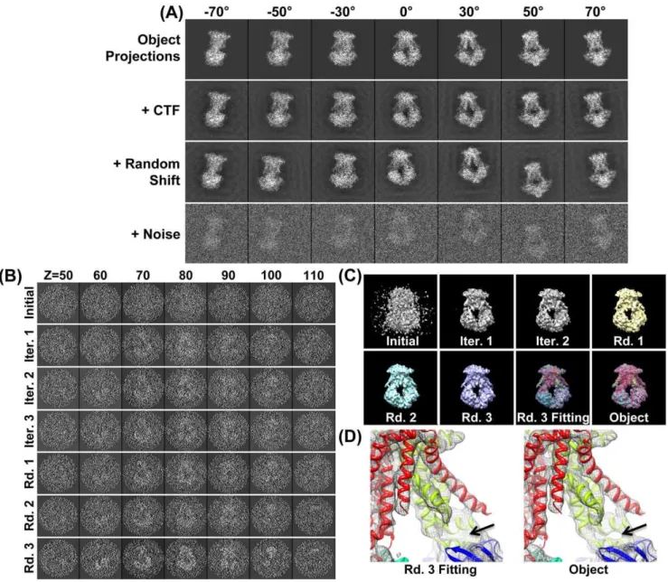
Figure 1. Simulating cryoET images and 3D reconstruction by IPET/FETR.(A) An object, a 3D density map of a single-instance protein (molybdate, portion of PDB entry 2ONK) was projected into a total of 141 tilt series of 2D images by following the simulated cryoET tilt-angles (containing both tilt-axis and tilt-angle errors in a range of60.5u), in which seven projections were presented (first row); to simulate contrast transfer function (CTF), CTF at a defocus of 1.5mm was applied to each image and then deconvoluted (second row); to simulate the translation errors, each image was randomly shifted with a maximal radius range of 30 pixels (third row); to simulate the noise, Gaussian noise (SNR = 0.2) was added to each image (last row). These images were used as the cryoET ‘‘raw’’ images for 3D reconstruction. (B) By FETR, the reference-free initial model was generated by directly back-projecting the ‘‘raw’’ images according to the measuring tilt-angles (containing immeasurable tilt-errors). The convergence of 3D reconstruction was approached by iterations through three major rounds. Selected ET slices of the 3D reconstruction of initial model, iteration one to three, round one to three, were displayed. (C) The isosurfaces of the corresponding 3D reconstructions were also displayed after they were low-pass filtered to 8 A˚ . The initial model displayed as a globular noisy blob, while the quality of reconstructions had been greatly improved after the 1–2 iterations. The reconstructions of each round contained many structural details, such as thea-helices. Docking the crystal structure into the isosurface from the final reconstruction displayed a near perfect match and no distinguishing differences from the object. (D) Zoom-in views of docked final reconstruction and object displayed slight difference as indicated by the arrows.
a lower defocus, CTF reversed the phases less frequently in reciprocal space than at a high defocus, and can provide more complete structural information for 3D reconstruction. For CTF correction, the CTF curve is deconvoluted from each simulated cryoET image by the ‘‘TF CTS’’ command in SPIDER software (Figure 1A) [21]. Although, the real cryoET experimental images at tilt angles contain a focus gradient across the image perpendicular to the tilt-axis, considering the image size we used is relatively small (160 A˚ in size) and the maximum defocus difference across the image is no more than,0.015mm under a tilt angle of 70u (the maximum defocus variation is less than
,1%) it is reasonable to ignore the defocus gradient across the image by using a common CTF curve in simulating cryoET images.
The particle centers in cryoET images normally do not overlap with the image centers. The difference between the particle center and image center is the translational error. To simulate translational errors, we randomly shifted particle centers within a radius of 30 pixels (Figure 1A). Considering that the image size was only 160 pixels, translational errors of up to 30 pixels are rather significant in the simulated cryoET images.
To simulate the noise in the cryoET images, Gaussian type noise was used, despite the limitations representing the noise as real cryoEM images. For instance, the variation in tilting angles produce different ice thicknesses that can result in a variation of signal-to-noise ratio (SNR) among the tilting images, while the different parts of the particle along the projection direction include different amounts of water molecules, resulting in an uneven distribution of SNR within an image. Although the variation of SNR among the tilting images can be minimized by an ‘‘exponential’’ exposure time scheme on a constant ice thickness area [23], the constant thickness of ice cannot be obtained in the real cryoET experiment. The uneven distribution of SNR within the image cannot be simulated by addition of Gaussian noise. Considering the sole purpose of using the simulation cryoET data is only for reporting a new reconstruction method, the Gaussian noise, a simple model, is chosen to roughly represent the noise in the cryoET images as that conventionally used in reporting the single-particle cryoEM reconstruction methods [20,22].
A Gaussian noise SNR of,0.2 is chosen and applied to all of the above simulated images, and since SNR = 0.2 it is within the range of our real cryoET experimental image measurement of 0.1–0.2 (the standard deviation (SD) of density measured by the SPIDER ‘‘fs’’ command, is,58.3–65.1 in the HDL particle area and is,53.7 in the background area) (Figure S2). To simulate
this SNR = 0.2 noise, a Gaussian noise with SD 5 times higher than the particle was added to each image (Figure 1A) using the ‘‘MO’’ and ‘‘AD’’ commands in the SPIDER software package [21,24].
The final simulated cryoET images (Figure 1A) contain geometric tilt-errors (including tilt-axis and tilt-angle errors) within 60.5u, translational errors within 630 pixels, high-level noise (SNR = 0.2), a missing wedge (tilt up to670u, the details of the missing-wedge effect to 3D reconstruction is discussed in Information S1) and CTF effects (defocus 1.5mm). Although the simulation has limitations in simulating real cryoET images, such as the defocus gradient, variation of SNR, the envelope function related to the particular EM instrument, the error in determination the CTF, and the real noise, the simulation data still has its value for verifying the program and evaluating the variation between the reconstruction and the known object considering that the simulation data will be used to demonstrate the reconstruction methodology only.
2. Basic tools for image processing basic tools
The IPET method/FETR algorithm includes an iterative refinement computational process. Each iteration contains several image-processing steps (Figure 2), such as generating the filter and mask to reduce noise, computing the new parameters for next iteration, and analyzing the 3D reconstruction variation/conver-gence. Some of the most important tools used are described below. Fourier shell correlation (FSC): To quantitatively analyze the variation and convergence of 3D reconstruction generated in each iteration, FSC analyses were used [25,26,27] in conventional single-particle reconstruction [20,21,28]. Instead of splitting the class averages into two groups in single-particle reconstruction, the raw ET images are split into two groups based on having an odd-or even-numbered index in the odd-order of tilt angle. Each group is used to generate a 3D reconstruction and then the two 3D reconstructions are used to compute the FSC curve over the corresponding spatial frequency shells in Fourier space (‘‘RF 3’’ command in SPIDER). Since this FSC computation uses a single set of ET images, we call it intra-FSC to distinguish it from the regular FSC computed between the 3D reconstruction and object. The frequency at which the intra-FSC curve falls to a value of 0.5 (called intra-f0.5) was used to represent the resolution of an iterated 3D reconstruction [20,21,29]. The intra-f0.5value will be used to generate related parameters in the next iteration (details described below).
Dynamic Gaussian low-pass filter: Our strategy to determine the translational errors/parameters is to use low-resolution information for initial searching, and then gradually use increasingly higher resolution information for further searching. To control the resolution information contributed by each iteration, a set of automatically generated Gaussian low-pass filters were used to reduce unnecessary structural details (Figure 2B). A series of 21 filters was used sequentially. A pair of boundary frequencies, the low-pass frequency (flow) and cut-off frequency (fcut), are defined as below, as
flow(i)~ 2 3|f0:5z
i
20|(fnyquist{ 2 3|f0:5),
fcut(i)~ 2 3|f0:5z
iz2
20 |(fnyquist{ 2 3|f0:5),
where i = 0, 1, …, 20. f0.5 is the intra-f0.5 defined in the previous iteration. Filters with increasingly higher pairs of boundary frequencies (i = 0,1,…,20) were used in subsequent iterations for progressively increasing high-frequency information and accuracy to determine the translational parameters. Notably, the filter is dynamic, as the filter boundary frequencies are a function of the intra-f0.5 value that is a reflection of the quality of 3D reconstruction in the previous iteration. If the reconstruction of the previous iteration converged well (i.e., intra-f0.5 moved to a higher frequency), the filter automatically moves to including higher-frequency image information during translational search-ing. In contrast, if the reconstruction converged poorly (i.e., intra-f0.5 moved to lower frequency), the filter automatically moves to include lower frequencies to increase the weight of low-resolution information during translational searching. As a result, the filter automatically corrects for poorly defined translation parameters in the previous iteration.
[20,31,32]. In the first round of our reconstruction iterations, a circular mask with a Gaussian edge was applied to each tilt image to reduce the effects of noise and remove excess background areas (Figure 2). The mask is generated based on the rough size and shape of the object. The mask should keep the intensity/density of raw image within object area, but reduce (not cut off) the density outside the object (mostly background noise). For example, a protein molecule with a size of roughly 100 pixels can generate a circular mask with a density value of 1.0 within a 120-pixel-diameter circle and density of 0.5 outside a 160-pixel-120-pixel-diameter circle (the largest circle that can fit in the image). The density value between these two circles is defined by the gradient of a Gaussian function.
Dynamic particle-shaped mask: A particle-shaped 3D mask and its projections (2D masks) were used to further reduce the noise and unnecessary background in iterations (Figure 2). In contrast to circular masks, the particle-shaped masks are generated based on the low-resolution structure of 3D reconstruction. The 3D reconstruction is filtered by a Gaussian low-pass filter based on the intra-f0.5value of the previous iteration. The density is modified as follows: a) the densities outside an isosurface (described below) are reset to 0.0, while densities inside the isosurface are reset to 1.0; b)
the modified density map is low-pass filtered to very low resolution (such as,60–80 A˚ ) to generate the particle-shaped mask (thus, the
densities near the mask boundary are modified as a gradient boundary by this low-pass filter). A total of six isosurfaces is used to generate the 3D masks that are sequentially used in the following iterations. The major difference among the masks is their isosurface containing space volume. The largest volume is defined as half the volume of the largest sphere that can fit within a box of 16061606160 voxels. The smallest volume is defined as three times the mass volume of the targeted protein molecule (the volume calculation is based on an estimated weight-to-volume ratio of 1.35 g/ml, i.e. 0.81 Da/A˚3[20]). Our experience was that a tight/small mask can reduce the noise efficiently, but an overly tight mask may result in truncation of the edges of targeted object. Thus, the smallest mask we used should be safe enough to avoid this truncation. The remaining four isosurface volumes are interpolated between those of the largest and smallest masks by the following rule: The inverse values of these four volumes are evenly distributed between the inverse values of the maximum and minimum mask volumes. The 2D mask that will be applied to a tilt image is generated by projecting the 3D mask according to a corresponding tilt angle of the tilt image, with one 2D mask Figure 2. Flow diagram of individual-particle electron tomography (IPET) method and focused electron tomography reconstruction (FETR) algorithm.(A) The IPET method contains two phases: the electron tomography (ET) data collection with image preprocessing, and a focused electron tomography reconstruction (FETR) algorithm. In the first phase, the single-instance of particle was imaged by ET. The contrast transfer function (CTF) of the whole-micrograph-size tilt images was determined, and then corrected after tilt images were aligned. The small images containing only a targeted particle were selected and windowed from each of tilt whole-micrograph, and then directly back-projected into 3D as the initial/starting model for refinement. The 3D reconstruction refinement procedure contains three rounds of refinement loops in the FETR algorithm. Each round was essentially the same, except different masks were applied. In the first round, a series of automatically generated circular Gaussian-edge masks was used; in the second round, the automatically generated particle-shaped masks were used and while, in the third round, the last mask in second round was used with association of an additional interpolation method during determining the translation parameters. (B) Each round of refinement loops contains the same iteration algorithm, FETR. 3D reconstruction from the previous iteration (or initial model for the first iteration) was projected, and the projections were used as references for the next iteration. Before translational parameter searching, a dynamic Gaussian low-pass filter and automatically generated mask were applied to both the references and tilt images.
applied to each tilt image. Since the 3D masks are generated by a Gaussian low-pass filter and the filter parameters are dependent on the intra-f0.5value of the previous iteration and the 2D and 3D masks depend on the convergence of the previous iteration (evaluated by the intra-f0.5value), we call these dynamic masks.
3. Focused electron tomography reconstruction algorithm
3.1 Image distortion and measurement tilt-errors are major obstacles in achieving high resolution in conventional electron tomographic reconstruction methods. Image distortion limits cryoET reconstruction resolution [33]. Image distortion has numerous causes, such as astigmatism [8], projector lens [34], pincushion and spiral [35,36], energy filter [9,10], and even radiation-induced deformations [11] along with defocus of non-parallel beam conditions. The distortion can result in measurement errors of tilt-axis and a tilt-angle that can never be eliminated.
Taking the example of defocus-introduced distortion, images under different defocus have slightly different magnification under non-parallel-beam EM operation conditions. To quantitatively demonstrate the change in magnification resulting from change in defocus, we imaged nanogold particles with a Gatan UltraScan 4 k64 k CCD camera equipped on a Tecnai 20 transmission electron microscope (Philips Electron Optics/FEI) operating at 200 kV. The 5 nm gold particles were deposited on the carbon-film coating on an EM grid. Tracking the coordinate changes of
,70 nanogold particles under defocus changes from 0.0mm to
10mm in steps of 0.5mm we were able to determine the changing ratio. In brief details, the micrographs under different defocus were aligned together based on their cross-correlation calculation (Video S1), and then the coordinates of,70 nanogold particles in
each aligned micrograph were fitted with a second-degree polynomial function by a least squares fitting method using MATLAB. The fitted parameters shown inTable S1suggest that, other than the constant numbers, a0 and b0, only two linear parameters,a1andb2have substantial change against defocus. By plottinga1and b2 against defocus, the distributions ofa1and b2 were similar to each other and flowing in a line, suggesting the particle coordinate change is nearly a linear relationship to focus change. Thus, a linear equation was used to fit thosea1andb2data and shown inFigure S3.The analysis showed that magnification changed ,8% as the defocus changed by 10mm (Figure S3).
Within a tilt image, the defocus is different only along the direction perpendicular to the tilt axis. The defocus difference can be as large as ,1.1mm from image edge to image center
(4096 pix65.6 A˚ /pix6tan(45u)/2) for a 4 k CCD image at a tilt-angle of 45u(imaged under a magnification of 20 kX with a pixel ratio of 5.6 A˚ /pix). The ,1.1mm defocus could result in a
maximum of ,0.85% distortion that corresponds to ,0.5u
measuring tilt-angle error. The calculation is based on the equation:Dh= cos21
[(1–0.85%)6cos(45u)]245u<0.5u(details dis-cussed in Figure S4). Similarly, other distortions can also introduce the tilt angle error in measuring tilt angles, and these tilt-errors can limit the reconstruction resolution when using whole micrographs.
The magnification changed by,8% when the defocus changed ,10mm as measured by our Tecnai T20 microscope under a
specific illuminatinga-angle condition (spot size = 7, illumination area is just covering the CCD size for a desired brightness and coherence beam). Note that the magnification change can be different depending on the microscope and illumination condition (including non-parallel beam, and even misalignment). For instance, using the T20 microscope under the parallel beam
condition, the magnification change can be less than 1%. However, the parallel beam condition does not fit to our desired condition in cryoET image acquisition because the beam is either too large in size, too weak in brightness or too poor in coherence (too large spot-size for a desired brightness). If the parallel beam is a necessary condition for cryoET imaging or the 8% defocus-related magnification change is defocus-related to misalignment of microscope, the experimental observation (Video S1, Figure S3 and Table S1) suggests the defocus-related magnification changes needs to be addressed during reconstruction, especially for high-resolution cryoET reconstruction. Our purpose in discussion of the defocus-introduced image distortion is to provide an example for many other image distortions (such as astigmatism, projector lens, pincushion and spiral, energy filter and radiation-induced deformations) to demonstrate how the image distortion can lead to a tilt-angle measurement error.
Conventional cryoET reconstruction methods call for using the whole micrograph for reconstruction [37,38,39,40,41,42] because it is believed that more signal in whole micrographs can provide more information for more accurate determination of the tilt-angle of each micrograph. We believe that image distortion limits the accuracy in determining the tilt-angles. The tilt-errors can directly affect the accuracy of the particle centers in whole micrograph reconstruction. Given the same tilt-errors, much less displacements occur near the reconstructing center than near the corner, and the reduction of displacement within the reconstructing subvolume, which yields a better quality 3D reconstruction. For example, a 0.5u error in tilt-axis will result in ,25-pixel (0:50=1800|
p|4096= ffiffiffi 2
p
) displacement error in the particle center at the corner of a 4 k64 k image, which will definitely induce errors in the reconstruction. In contrast, the 0.5uerror in tilt-axis will result in less than 1.6-pixel (0:50=1800|p|256= ffiffiffi
2
p
) displacement error in the particle center at the corner of a 2566256 pixel small-image, which will induce much less error in the 3D reconstruction. A similar experience in the cryoEM single-particle reconstruction is the reconstructed subvolume near the central area has generally better quality than far from the center (i.e. corner and edge areas). More detailed discussion about how tilt-error affects the cryoEM 3D reconstruction is given in subsection 1 of Discussion Section. According to the above statements, we developed this IPET/ FETR to limit the effects from tilt-error by reducing reconstruc-tion image-size to a small size that includes only a single-instance protein particle for 3D reconstruction.
majorly among tilt images. Although the tilt-anglehcan be read from the goniometer of the microscope or measured by tracking the movement of fiducial markers, neither of the methods can provide an accurate value for h, as h must contain an error resulting from the image distortions described above. A conservative estimate of the tilt-angle error is similar to tilt-axis error, i.e. within a range of 60.5u, so we used these ranges to generate simulated cryoET images. Our tomography reconstruction strategy in reducing the adverse effects from the tilt-errors (tilt-axis and tilt-angle errors) is to reduce the reconstruction image size by including only the targeted particle, hence the name: focused ET reconstruction (FETR) process, where only two translation parameters (Dx andDy) need to be defined.
The key procedure in FETR is to accurately determine the translational parameters (Dx and Dy) of each particle in each image that is precisely aligned to a global center (Figure 2). The 3D reconstruction obtained from the previous iteration (or initial model) is tilted and projected by the measured tilt-angles (that contain immeasurable errors). The generated projections are used as the references to search for the translation parameters (Dx and Dy) by a reciprocal space cross-correlation calculation (‘‘CC N’’ command in SPIDER). Notably, each projection is used only once as a reference for the tilt image that shares the same tilt-angle. Prior to searching, a dynamic filter and a mask were applied to both the references and the tilt images.
Three rounds of refinement (the coarse refinement round, the fine refinement round, and the oversampling refinement round) were used to determine two translation parameters (Dx andDy) (Figure 2). Each round contains multiple iterative refinement procedures as described below.
3.3 Focused electron tomography reconstruction. Gener-ating a reference-free initial model is necessary to start the iterative refinement. A reference-free initial model was generated from the raw (original) ET images themselves by a reciprocal space back-projection algorithm (‘‘BP 3F’’ command in SPIDER). The reference-free initial model in ET slices displayed a noisy reconstruction with no obvious structural details, except a slightly higher density region near the center (Figure 1B). Its isosurface showed a central globular blob with a noisy surface and suggested no useful structural information other than the rough size of the object (Figure 1C). The intra-FSC analysis of the initial model showed that the value of intra-f0.5was,1/40 A˚21(Figures 3B and S5A). The first round is a coarse refinement with circular masks and dynamic filters. In this round, a total of 21 dynamic Gaussian low-pass filters and a set of circular Gaussian-edge masks were automatically generated and applied to both the reference and tilted image.
In the first iteration, we generated the references by projection from the initial model, and then we applied the first Gaussian low-pass filter (i = 0) and the circular mask to both the references and raw images to compute their cross-correlation peaks to determine the translation parameters of each raw image (Figure 3A, top left corner). The determined translation parameters (after rounding to integers in order to avoid the error from interpolation) were applied to the corresponding raw images to generate the first-iteration 3D reconstruction (Figure 1B and 1C). The translation-shifted raw images were split into two groups and used to generate two independent 3D reconstructions to compute the variation and determine the first-iteration intra-f0.5 value (Figure 3B, blue points). The intra-f0.5value was used for the related parameters to generate the second-iteration filter (i = 0). A further analysis of the convergence was to calculate the mean of the translation parameters (before rounding) in the current iteration. The
translation mean, 14.45 pixels/image, suggested that the first iteration had dramatically recovered error in the particle centers (Figure 3A). Thus, it was not surprising that the first-iteration 3D reconstruction revealed the overall shape of the object (Figure 1B and 1C).
The second iteration was essentially the same as the first iteration, except for i) using the first-iteration 3D reconstruction rather than reference-free initial model to generate the references; and ii) using the first-iteration intra-f0.5to automat-ically generate the second-iteration filter parameters by the equations shown in the subsection 2 of Methods Section. Although the second-iteration filter (i = 0) equation was identical to that of the first iteration, the second-filter parameter intra-f0.5 was modified by the first-iteration intra-f0.5instead of the initial intra-f0.5, which normally allows for better resolution. The second-iteration filter would actually include more high-resolu-tion informahigh-resolu-tion during the second iterahigh-resolu-tion. The determined translation parameters (after rounding to integers) were used to generate the second-iteration images and 3D reconstruction (Figure 1B and 1C). The second-iteration 3D reconstruction had no obvious visual difference from the first-iteration 3D reconstruction after both 3D reconstructions were filtered to 8 A˚ . However, analysis of the intra-f0.5 value suggested the second-iteration reconstruction had better resolution and significantly less variation than the first-iteration reconstruction (Figure 3B, blue points).
We repeated the above iteration procedure a minimum of four times until the change of translation mean was below 0.01 pixels per image (termination criteria). After the 13th iteration, the change had decreased dramatically from 14.45 pixels to below 0.01 pixels for the first time (Figure 3A). The iteration process was restarted with more high-resolution information by automat-ically replacing the first filter (i = 0) with the second filter (i = 1) and using a finer Gaussian low-pass filter. The iterations hit the termination criteria again after 17th iteration, during which the change dropped to below 0.01 pixels (Figure 3A).
Iteration continued through low-pass filters, including higher and higher resolution structural information. However, past a certain point, higher-resolution information does not necessarily contribute to greater accuracy in determining the translational parameters. The same termination criteria (,0.01 pixel per image) were used after the first three filters were used. In this round, a total of 21 iterations were conducted before hitting the termination criteria (Figure 3A).
The ET slices of the 21st-iteration 3D reconstruction displayed a clear density in the center slices (Figure 1B). The isosurface of the 3D reconstruction (after filtered to 8 A˚ ), at the contour level that contains a volume equal to the initial model volume (70% space volume of the protein molecule, at which level the secondary structure could clearly be seen), showed significant structural detail, such as a hole and somea-helices (Figure 1C). Intra-FSC analysis showed that intra-f0.5 improved significantly (from 1/ 40 A˚21
to 1/16.6 A˚21
) (Figure 3B, blue points). This analysis suggests that the 3D reconstruction gradually converged and the translation parameters were determined precisely.
In this round, a total of six particle-shaped 3D masks were generated and applied sequentially from largest volume to smallest volume (Figures 3Atop panel andS6). Other than the difference in shape among the 3D masks, the major difference among the masks was their space volumes. Their mask volumes corresponded to protein molecular weights of 800 kDa, 600 kDa, 480 kDa, 400 kDa, 340 kDa, and 300 kDa (Figure S6). These mask volumes were chosen such that the inverse numbers of these volumes were evenly distributed.
(Figure 1B). The 3D reconstruction showed more structural detail than the reconstruction from the first round (Figure 1C).
The translation mean changes demonstrated that these masks were very effective for translation parameter determination. However, the masks should be monitored and confirmed that no portion of the particle was truncated (Figure S6). Although the last 3D mask contained the smallest volume (3 times the object volume) (Figures 3A and S6), considering the iteration nearly converged (the average change was significantly below 1.0 pixel/ image), this mask is still safe to be used.
The third round is an oversampling refinement. In the above two rounds, the translation parameters were converted to integers before being applied to the images. This was important in order to avoid the error introduced from the multiple interpolations. However, the accuracy of determining these translation param-eters was also limited by the use of integer values. In this round, we released the integer restriction by using an oversampling technique to further improve the reconstruction (Figure 2). Expansion of the image size by 10 times in each dimension was performed using the triangular interpolation technique (‘‘IP T’’ command in SPIDER), and then continued through the iterations following the last iteration of the second round (Figure 3A, top right corner). In this process, the corresponding 2D masks were also interpolated by 10 times before being applied to the expanded references and the images prior to determine the translational parameters. To avoid computer memory overflow, the images and masks were shrunk by a factor of 5 in each dimension before back-projection. We repeated this iteration seven times until the change of translation mean between two successive iterations was below 0.001 pixels/ image.
The center ET slices of the final 3D reconstruction showed significantly better contrast than the last reconstruction from the second round (Figure 1B), despite intra-FSC analysis showing no obvious improvement in the intra-f0.5 value (Figure 3B). The isosurface of the last 3D reconstruction (after filtered to 8 A˚ ) displayed many more important structural details (Figure 1C and 1D) than that of the last reconstruction of the second round, suggesting that the reconstruction had achieved further improve-ment with the oversampling technique.
Results
1. Variation analysis of the FETR reconstruction of simulated cryoET data
Variation analysis was conducted from two aspects: translation-al parameters and 3D reconstruction. To antranslation-alyze the deviation of translation parameters from their ‘‘ideal’’ centers, we calculated the difference between the ideal center (Figure 1A) and the center defined from IPET/FETR. A variation analysis of these ‘‘absolute translation errors’’ was performed by displaying each absolute translation error of each image against its image index. The distribution showed the absolute translation error in the initial raw images was distributed evenly in the range of 30 pixels with a mean of 14.96 pixels/image (Figure 3D, gray line). However, after the first round, the absolute translation error was significantly reduced to a mean of 1.72 pixels/image (Figure 3D, green line). After the second round, the absolute translation error continued to be reduced to a mean of 0.71 pixels (Figure 3D, purple line), and was reduced further to a mean of 0.46 pixels after the third round (Figure 3D, blue line). This analysis suggests that the absolute translation error was gradually minimized.
A further variation analysis of absolute translation error was performed by computing the histogram. The histogram showed that ,95% of the images had a translation error below ,3.5
pixels/image after the first round, reduced to,1.4 pixels/image,
and further decreased to below,1.0 pixels/image after the second
and third round, respectively. In the process, the peak population is ,4.87% with an error of ,1.48 pixels/image after the first
round (Figure 3E, green dotted line), which increased to
,11.70% with a smaller error of ,0.68 pixels/image
(Figure 3E, purple dash-dot line), and further rose to,15.72%
with an even smaller error,,0.34 pixels/image (Figure 3E, blue solid line) after the second and third round. Both the above analyses suggested that the variation of the translation parameters was relatively low after the three rounds of iterations.
Variation analysis of 3D reconstruction was also conducted by methods: Fourier space FSC analysis and real-space cross-correlation analysis. In Fourier space analysis, the FSC curve between each 3D reconstruction (Figure 1C) and the ideal object was computed, and was further used to determinef0.5value. The f0.5distribution showed that: i) in the first iteration, even though thef0.5value was,1/40 A˚21(consistent with the intra-f0.5value),
the initial model had little similarity with the object (Figure S5B, gray circle-dash line) except for roughly correct dimensions (Figure 1C); ii) in the last iteration of the first round, thef0.5 value had quickly improved to beyond,1/14 A˚21(Figure 3B,
purple circles) and the 3D reconstruction showed significantly more similarity to the object (Figure S5B, green diamond-dash line) and contained many structural details, such as the central hole and somea-helices (Figure 1C); iii) in the second and third rounds, thef0.5value further improved to beyond,1/11 A˚21. 3D
reconstructions of the object also showed further improvement (Figure S5B, purple cross-dash line and blue point-dash line). The 3D reconstruction contained more structural details than that of the first round, and remarkably showed almost alla-helices that had emerged, suggesting that the 3D reconstruction had converged to the object (Figures 1C and 1D). The intra-f0.5 value showed no significant improvement after the first round (Figures 3Bblue points andS5A), but thef0.5value calculated between the 3D reconstruction and the ideal object showed significant improvement after the first round. This suggests that the intra-f0.5value was not sensitive enough to be used for defining the 3D resolution or used as an iteration termination criterion. For this reason, we used the change in translation mean error as the termination criterion.
To minimize the mask effect on FSC calculation in the variation analysis, we used the circular-shaped mask with density-gradient boundary instead of the particle-shaped mask. The outer diameter of the circular mask equaled the size of image. The special particle-shaped mask was only used for searching for the translational parameters. Despite the mask enhancing the intra-FSC correlation, the resolution calculated from the circular-mask-applied images was significantly lower than the resolution calculated from the FSC between the reconstructed 3D map and object. Namely, even the circular mask generated an overly optimistic correlation; the resolution is still much poorer than the real resolution of the 3D map should be.
before calculating CC C, these CC C values were increased significantly (Figure 3C). In summary, both variation analyses showed that the iteration robustly corrected the translational errors and improved the 3D quality during iterations and refinements even when the immeasurable tilt-errors exist.
2. Validation of the focused ET reconstruction method by real experimental data
2.1 3D reconstruction of an antibody by negative-staining ET. To validate IPET method and FETR algorithm, we applied this method to a set of real experimental data, with antibody negative-staining (NS) images. The antibody is naturally dynamic, fluctuates frequently and is structurally heterogeneous. The structural heterogeneity makes the study of the structure and function difficult using current technologies such as x-ray crystallography, nuclear magnetic resonance (NMR), and even EM single-particle reconstruction because all of these techniques need the average signal from thousands to millions of individual particles. One of the features of our IPET method is that the 3D reconstruction is from an individually targeted, single-instance of molecule/protein that is free of conformational dynamics and heterogeneity. The 3D structure can be treated as a ‘‘snapshot’’ of the dynamic structure.
The human IgG antibody (molecular weight: ,150 kDa)
sample was prepared with an optimized NS protocol [45,46], and imaged using the ET technique on an FEI T20 microscope under 80 kX magnification and defocus of less than 2mm [18]. By tracking and windowing a targeted single-instance of an antibody particle from each tilt micrograph after CTF correction by TOMOCTF [47], we reconstructed its 3D density map
(Figures 4andS7, S8, S9, S10) with our IPET method/FETR algorithm. To further validate the method, we windowed the images of another targeted single-instance of antibody particle and reconstructed it into 3D (Figures 4andS7, S8, S9, S10). The 3D density maps contained rich structural details (Figures 4B and 4E), including the shape of each domain, and even the holes inside each domain. Intra-FSC analysis showed that the resolution was ,15 A˚ (Figure S9). Note, the actual resolutions were generally much better than that defined from the intra-FSC described in subsection 1 of Results Section. Although the resolution from intra-FSC is not as high as what we achieved in the simulated cryoET image, the resolution is, as far as we know, the highest resolution map ever obtained by tomography reconstruction.
Since a NS image involves a coating stain and the shape of the coating stain represents the surface structure of protein, we asked if the resolution measurement represented information on the protein rather than just good resolution of the stain structure. The NS protocol used in preparation of the antibody sample is from our recently published optimized protocol [45,46], and we demonstrated that with our protocol, we could generate lipoprotein particles that have similar size and shape to that of cryoEM [45,46]. All three domains of antibody show the same sort of hole in the middle—two holes are similar in size, but one hole is obviously bigger than other holes. The holes have been revealed by the crystal structure of the IgG antibody. Displaying the crystal structure of the IgG antibody (PDB entry 1IGT) by two methods— the ribbon and Van der Waals surface—both views show holes in the Fab domain (Figure S11, the top two domains) and the Fc
domain (Figure S11, the bottom domain). Remarkably, the Fc
Figure 4. 3D reconstructions with negative staining of an IgG antibody by IPET.(A) A single-instance of an IgG antibody was imaged by negative staining (NS) ET. Nine tilted views of the same single IgG particle were selected from 81 tilt micrographs that were CTF corrected by TOMOCTF, and then displayed in leftmost column. By FETR algorithm, the 3D reconstruction was iterated and converged. The corresponding tilting projections of the 3D reconstruction from major iterations were displayed beside the raw images in six columns. (B) The final 3D reconstruction of a targeted individual antibody particle was displayed in a contour level that contained a volume corresponding to 160 kDa. The reconstruction displayed three ring-shaped domains that corresponding to three domain of IgG antibody. (C) Docking the crystal structure (PDB entry 1IGT) of each domain of the IgG antibody into each ring-shaped density of IgG showed a good fit. The docking was performed by a rigid-body docking option in Chimera program [79]. The loops between the domains were simply connected by Chimera. (D) Another example of the IPET method in a 3D reconstruction of another single-instance of a targeted individual IgG antibody particle. The NS-ET images of the raw images and projections of the related reconstruction were also displayed. (E) The 3D reconstruction of this antibody particle displayed a similar structural feature to the first one, such as the three domains. (F) Docking the IgG antibody crystal structure into the density map showed a good fit as well.
domain hole is much bigger than the holes in Fab domain,
consistent with our 3D reconstruction.
To determine further if the holes were artifacts of defocus-related CTF, we imaged the antibody sample under Scherzer focus condition. The survey NS image (after filtered) and selected particles show the holes in all three domains can obviously be visualized directly (Figures S12A and S12B), and the corre-sponding holes can also be visualized from the crystal structure under similar orientation (Figure S12C). Thus, the holes were less likely caused by CTF artifacts. The NS image suggested our stain of uranyl formate (UF) can penetrate the protein surface and display the internal structure. This result was consistent with our observation in lipoproteins [45,46], but challenged the conven-tional wisdom and concept that negative staining can only show the surface structure information of coated proteins.
Despite the detailed structure of the holes, the spatial and orientation relationships among the domains are reliable. The 3D reconstruction from single-instance antibody that is free of conformational dynamics and heterogeneity can be treated as a ‘‘snapshot’’ of the dynamic structure of antibody. By comparing these ‘‘snapshot’’ IgG antibody structures, this method could allow us to study antibody dynamics. For example, by aligning two docked PDB files by aligning their Fcdomain, the Fabdomains are
different from each other in location and orientation, suggesting the equilibrium fluctuation and structural dynamic character of IgG antibody (Figures 4C and 4F,Video S2).
2.2 3D reconstruction of high-density lipoprotein by cryoET. To further validate our method on high-noise real cryoET experimental data, we applied this method to the structure determination of nascent high-density lipoprotein (HDL) [16,17]. A nascent HDL sample was prepared as described [15,45,48,49]. HDL particles in vivo vary in size, shape, components, and
biological functions [15,45,48,49,50]. A particular component of these, called nascent discoidal HDL (molecular weight: 140– 240 kDa) is the disk-shaped precursor of mature spherical HDL and contains phospholipids, and 2 to 3 apolipoprotein A-I (apoA-I, molecular weight: 28 kDa) molecules per particle. This kind of discoidal HDL is a critical intermediate between lipid-poor apoA-I and mature spherical HDL during HDL assembly. However, HDL structure determination is complicated by the dynamic nature and heterogeneity of HDL [15,45].
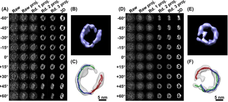
By IPET method, we used the cryoET technique to image the nascent HDL particles that were embedded in vitreous physio-logical buffer (Figure S2) under defocus of,1.5mm as described [15]. This sample contained 17 nm nascent HDL particles. To demonstrate the effectiveness of the FETR algorithm, we targeted two 17 nm nascent HDL particles for 3D reconstruction (Figures 5 and S13, S14, S15, S16). We focused on the 17 nm HDL particle because the 17 nm HDL is the only HDL fraction that has been investigated by cryoEM [51]. Dr. van Antwerpen’s group examined the 17 nm HDL particles embedded in vitreous ice from orthogonal tilt views and found that the 17 nm HDL particle has a discoidal shape (Figure S17) [51].
The cryoET images of the targeted 17 nm rHDL particle were manually windowed from CTF-corrected (by TOMOCTF) cryoET micrographs [47]. The particle images were noisy, but the particles could be visualized (Figure 5A and 5D). Using FETR, the particle centers were precisely aligned to their ‘‘global center’’ by associating them with a series of automatically generated masks. To ensure the particle-shaped masks in the second round of FETR did not cut off any portion of the particle, the raw particle images were monitored after masks were applied (Figure S16). The slices of the 3D reconstruction were also monitored before and after we applied low-pass filters and/or
Figure 5. 3D reconstructions of a cryoET 17 nm nascent HDL particle by IPET.(A) An individual targeted nascent HDL particle embedded in vitreous ice was imaged by the cryoET technique. The tilt images of a targeted particle were windowed from the tilt series of cryoET micrographs after the CTF was corrected by TOMOCTF. Nine represented tilted views of a targeted 17 nm HDL particle were shown in leftmost column. These selected tilt images were from 81 tilt micrographs that were taken at the specified tilt angles. The other six columns in each grid showed the results of progressive refinement from certain iterations. (B) Reconstructed to 3D density map. The high-density portion corresponding to proteins, apolipoprotein A-I (apoA-I), was formed in a ring shape. (C) By docking the double-helices into the ring-shaped density, the size suggests three apoA-I molecules exist in a 17 nm HDL particle. (D) Another targeted 17 nm HDL particle was imaged and reconstructed for 3D density map. (E–F) The 3D reconstruction showed the similar structural feature to the first HDL particle, suggesting our cryoET reconstructions are consistent as reported by cryoEM observation [51].
masks (Figures S13A, S13B, S13C, S13D, S14A, S14B, S15,S14D). Although the slice views are very noisy, such as with the central slice (Z = 50 shown in Figure S13A, and Z = 100 shown inFigure S14A), by simply applying a low-pass filter (50– 60 A˚ ), the particle immediately stood out from the background while the noise was immediately reduced (shown in Z = 50 of Figure S13B, and Z = 100 ofFigure S14B). This was due to the noise presented in the slice is high-frequency noise. This low-pass filtered 3D was then used to generate the particle-shaped mask with a volume of ,3–8 times greater than the HDL molecular
volume by following same procedure as described in subsection 2 of Methods Section. By applying this mask on the 3D reconstruction, the projections of the 3D reconstruction had significantly higher SNR (the 4thpanel shown inFigure 5A and 5D). The improvement of SNR in projections was due to the cut-off of these noises that were originally overlapping with the particle along the projection direction, but not overlapping in 3D space. To ensure the final mask did not cut off the particle, the final 3D reconstructions before and after applying the final mask were displayed (Figures S13EandS13F, andS14EandS14F). Only a few small isolated densities were excluded by the final mask (shown in gray,Figures S13EandS14E).
By FETR, the noise in the final 3D projections was rapidly eliminated and the particle signal was quickly enhanced (Figure 5A and 5D). Both final 3D reconstructions (Figure 5B and 5E) displayed many common features, such as a discoidal shape and a density portion in the form of a ring. The high-density portion in the high-density map corresponds to the high-high-density component of HDL, i.e., apolipoprotein A-Is. It is commonly believed that apoA-I forms a double-helical bundle that wraps around the hydrophobic portion of the lipid bilayer in HDL [15,52]. Two helices in the ring-shaped density cannot be distinguished from the reconstructions because their center distance is only,10 A˚ .
Although the intra-f0.5defined resolution is usually lower than the actual resolution (discussed in the subsection 1 of Results Section), the intra-f0.5 defined ,36–42 A˚ resolutions of nascent
HDL maps (Figure S15) are not different from the resolution obtained by conventional cryoET methods. However, considering that nascent HDL particles have molecular mass,200 kDa and
,200 kDa protein particles are rarely successfully reconstructed
by even the single-particle reconstruction method, the successful reconstruction of a 3D density map of a single-instance,200 kDa
HDL particle is remarkable. The anti-parallel a-helices formed into a ring-shape from cryoET is amazingly consistent with the structures i) shown in the raw cryoET images of nascent HDL particle (Figure S2) [15], ii) shown in conventional cryoEM images that acquired from two orthogonal tilted angles reported by van Antwerpen (Figure S17) [51], and iii) the structural model derived from the energy minimization by molecular dynamic simulations [15,52], suggesting that our IPET method/FETR algorithm is a powerful tool for cryoET reconstruction. We believe that, by further optimizing the cryoET imaging conditions to more closely match the simulated cryoET conditions, a higher resolution structure of a single-instance nascent HDL can be expected.
Despite the resolution, the 3D reconstruction from a single-instance HDL particle that is free of conformational dynamics and heterogeneity can be treated as a ‘‘snapshot’’ of the dynamic structure of protein. By comparing these ‘‘snapshot’’ HDL structures, this method could allow the study of HDL structural dynamics. By aligning two docked PDB files, the differences between two structures in location and orientation suggested the equilibrium fluctuation and the structurally dynamic character of the HDL particle (Figure 5C and 5F,Video S3).
Discussion
1. Image distortion limits high-resolution 3D reconstruction by conventional tomography reconstruction methods
The conventional method for ET reconstruction is to use the large micrograph-size images for more accurate determination of geometric tilt-angles and translation parameters [37,38,39,40, 41,42]. Unfortunately, the resolution of 3D reconstruction from these methods has rarely been better than 30 A˚ . It has been reported that image distortion limits reconstruction resolution [33]. As mentioned above, the image distortion could have numerous causes, such as defocus (details in subsection 3.1 of Methods Section), astigmatism [8], projector lens [34], pincushion and spiral [35,36], energy filter [9,10], and even radiation-induced deforma-tions [11]. We suspected that image distortion prevents the accurate determination of tilt-angle, further limiting high-resolution recon-struction from large micrograph-size tilt images by conventional cryoET reconstruction. As described in subsection 3.1 of Methods Section, defocus-related distortion could result in,0.5utilt-angle
measuring error on a 4 k CCD under 20 kX magnification. To demonstrate how tilt-error effects 3D reconstruction, we built up a large object that contains evenly distributed identical protein (Figure S18) and used it to project a set of 141 simulated micrograph-size noise-free images (,4 k64 k pixels) containing tilt-errors (both tilt-axis and tilt-angle errors) in a range of60.5u
(Figure S1). By back-projecting the set of projection to 3D reconstruction, the 3D reconstruction contained evenly distributed particles (Figure S18), but, the quality of the particle reconstruc-tions varied dramatically in term of the distance of a particle from the center of the full-size image (Figure S18 and S19A). The particles near the center of the 3D reconstruction closely resembled the actual object, while those at the corners were least similar (Figure S18 and S19A). To quantitatively evaluate the quality of each reconstructed particle against its spatial location, an FSC curve and CC C value between each reconstructed particle and object was computed. By plotting thef0.5and CC C values of the particles against their in-plane locations, both distributions showed a sharp peak at the center area, suggesting that only the particles/subvolumes near the center of reconstruction area were most similar to the object (Figure S19B).
To further examine the effects of smaller angle errors on a reconstruction, we repeated the above test using a smaller angle error (within a range of 60.1u instead of 60.5u). The particles near the central area were still the most similar to the object (Figure S19C), while the particles near the edges and corners consistently showed reduced similarity to the object (Figure S19C). F0.5 and CC distributions had center peak areas significantly larger than those from the previous test (Figure S19D), suggesting a relatively larger area of high-resolution reconstruction. Both tests demonstrated that the geometric angle error grows with increasing displacement from the particle center and has uneven influence on the reconstruction quality, with the area near the reconstruction center having the highest reconstruc-tion resolureconstruc-tion.
correlation value under the larger tilt-axis errors (60.5u) than under the smaller errors (60.1u), suggesting that the central subvolumes/particles can tolerate a higher level of tilt-axis measurement error.
For a better understanding of the effect from tilt-angle error alone, we also repeated above tests with only the tilt-angle random errors in a range of 60.5u (Figure S21A) and60.1u (Figure S21B). Both tests also showed that the particles/subvolumes along the tilt-axis had the best similarity to the object, while the particles/subvolumes far from the tilt-axis had the least similarity to the object based onf0.5and CC analyses. The distribution had a much narrower mountain ridge with a similar high correlation value in the larger tilt-angle errors test (60.5u) than the smaller error test (60.1u) (Figure S21), suggesting that the subvolumes/ particles along the tilt-axis can tolerate a higher level of tilt-angle measurement error.
Although one of reasons to add the measurement errors of tilt-angle is the image distortion by different defocus values under non-parallel illumination condition, non-parallel illumination could be achieved by using a FEI Titan Krios microscope and a Zeiss Libra microscope, which could eliminate the defocus-related distortion. However, one cannot declare that there are no tilt-angle measurement errors for the tomographic data set collected from these microscopes.
Generally believed, the accurate tilt-axis orientation determi-nation is very important for good ET reconstruction by conventional whole-micrograph tomography reconstruction meth-ods. Among the three Euler angles in tomography reconstruction, the first Euler angle w (particle angle) is equal to zero and not important. The offset value for the third Euler angleh(tilt angle), which is important for the whole specimen section reconstruction by using ART [53] or the SIRT method [54], is also not important for conventional single-particle reconstruction because it only needs relevant angles. Does the second Euler angle y (tilt-axis angle) take effect with individual particle tomography? The tilt-axis errors include two types of error, the random error (we have discussed in above) and systemic error (because not all the microscopes could be pre-aligned well and will yield a none-zero tilt-axis angle within a range of ,1u–5u). For a better
understanding of the effect from the systemic angle-error of tilt-axis alone, we repeated the above test by only introducing a fixed systemic tilt-axis error of 1.0u(no any other errors included). By same analysis, thef0.5distribution showed a center peak (Figure S22A), suggesting that only the central subvolume had the highest similarity to the model, while the subvolumes along the tilt-axis direction are generally better than those against tilt-axis direction. The FSC curve (Figure S22B, blue line) between the model and the center subvolume showed the center subvolume (Figure S22C) retains its high similarity to the model with a resolution much better than 10 A˚ . By increasing the tilt-axis systemic error to 5.0uand even 10.0urespectively, the FSC curves (Figure S22B, purple and green lines) showed the center subvolume (Figure S22DandS22E) still retains its high similarity to the model at a resolution up to 10 A˚ . After low-pass filtering to 8 A˚, all three central subvolumes are highly similar to each other in shape, but at a different tilt (Figure S22C–S22E). These tests suggest the tilt-axis orientation determination is very important for good ET reconstruction by conventional tomography reconstruction meth-ods, but not important for our FETR algorithm. In other words, our FETR algorithm can tolerate a high tilt-axis systemic error (10u), while conventional whole-micrograph reconstruction can-not.
Whether the,0.5uangle measurement error is realistic or not,
the existence of image distortion and tilt-error drove us to develop
this FETR algorithm to tolerate these image distortions and measuring angle errors for high-resolution cryoET reconstruction.
2. Roughly 100 high-noise images are sufficient for a 3D reconstruction at intermediate resolution
In our cryoET reconstruction, a mere 100 high-noise images were sufficient to achieve intermediate resolution (1–2 nm); in contrast, single-particle reconstruction requires thousands of images to achieve the same resolution. As such, we asked whether
,100 high-noise images are sufficient for a 3D reconstruction at
an intermediate resolution. To address this question, we conducted the following simulation. We generated a set of 84 projections by rotating and projecting an object from a set of 84 geometric Euler angles generated from the single-particle reconstruction method under a space-sampling angle of 15u
(‘‘VO EA’’ command in SPIDER). Then, we added eight different levels of Gaussian noise with SNR ranging from noise-free to 0.1 to each set of projections (Figure S23A, S23B, S23C). This noise range covers the noise levels often present in cryoEM images [55,56,57]. To demonstrate the effect of noise level on 3D reconstruction, we back-projected eight reconstructions from each set of images with the assumption that all five parameters in each image were perfectly defined (Figure S23D, S23E, S23F, S23G). Although perfectly defining all parameters is impossible in practice, it is a necessary test to distinguish whether the resolution of a 3D reconstruction is limited by the noise level or other reasons. All eight density maps reconstructed from eight different noise levels (SNR = 0.1, 0.2, 0.3, 0.4, 0.6, 0.8, 1.0 and noise-free) were analyzed by two methods: FSC and CC analysis, which both analyses showed that the noise was reduced, and the reconstruc-tions were similar to each other at a resolution close to or better than 10 A˚ (indicated by f0.5 values) (Figure S23H). These structural details suggest that a set of 84 high-noise images (SNR = 0.1) would be sufficient for a reconstruction at interme-diate resolution if all five parameters in each image can be perfectly defined.
Similar discussion about the minimum number of projections needed for a 3D reconstruction with a specific resolution has already been discussed by Crowther et al. [58,59,60]. Based on their equation, for the diameter of the molybdate transporter of
,100 A˚ , the minimum number of projections for a reconstruction
with,10 A˚ resolution is given byp6100 A˚ /10 A˚ = 31.
Consid-ering the calculation is based on noise-free projections, the minimum number of the noise-including projections should be higher than 31. The above simulation suggested that a set of 84 high-noise images (SNR = 0.1) would be sufficient for a recon-struction at intermediate resolution if all five parameters in each image can be perfectly defined. However, considering the accuracy of five parameters is critical plus the Gaussian noise has limitation in simulating the noise in cryoEM (discussed in subsection 1 of Methods Section), the minimum number of real experimental noise images is difficult to determine.
Another question posed is what results in real single-particle reconstruction often requiring thousands of particle images to achieve intermediate resolution [61]. We believe it is because the class-average process was used in single-particle reconstruction. To determine all five parameters, class-averaging procedure is often used to generate high-contrast class averages. With a typical single-particle reconstruction, a class average that contains ,10–20
images and a sampling angle is usually between 5.0u and 10.0u, 173–711 class averages corresponds to a total of,1,730–14,220