Hydrol. Earth Syst. Sci., 17, 1331–1363, 2013 www.hydrol-earth-syst-sci.net/17/1331/2013/ doi:10.5194/hess-17-1331-2013
© Author(s) 2013. CC Attribution 3.0 License.
Geoscientiic
Geoscientiic
Hydrology and
Earth System
Sciences
Open Access
Estimating actual, potential, reference crop and pan evaporation
using standard meteorological data: a pragmatic synthesis
T. A. McMahon1, M. C. Peel1, L. Lowe2, R. Srikanthan3, and T. R. McVicar4
1Department of Infrastructure Engineering, The University of Melbourne, Parkville, Victoria, 3010, Australia 2Sinclair Knight Merz, P.O. Box 312, Flinders Lane, Melbourne, 8009, Australia
3Water Division, Bureau of Meteorology, GPO 1289, Melbourne, 3001, Australia
4Land and Water Division, Commonwealth Scientific and Industrial Research Organisation, Clunies Ross Drive,
Acton, ACT 2602, Australia
Correspondence to:T. A. McMahon ([email protected])
Received: 19 September 2012 – Published in Hydrol. Earth Syst. Sci. Discuss.: 18 October 2012 Revised: 26 February 2013 – Accepted: 14 March 2013 – Published: 10 April 2013
Abstract. This guide to estimating daily and monthly ac-tual, potential, reference crop and pan evaporation covers topics that are of interest to researchers, consulting hydrol-ogists and practicing engineers. Topics include estimating actual evaporation from deep lakes and from farm dams and for catchment water balance studies, estimating poten-tial evaporation as input to rainfall-runoff models, and refer-ence crop evapotranspiration for small irrigation areas, and for irrigation within large irrigation districts. Inspiration for this guide arose in response to the authors’ experiences in reviewing research papers and consulting reports where es-timation of the actual evaporation component in catchment and water balance studies was often inadequately handled. Practical guides using consistent terminology that cover both theory and practice are not readily available. Here we pro-vide such a guide, which is dipro-vided into three parts. The first part provides background theory and an outline of the con-ceptual models of potential evaporation of Penman, Penman– Monteith and Priestley–Taylor, as well as discussions of ref-erence crop evapotranspiration and Class-A pan evapora-tion. The last two sub-sections in this first part include tech-niques to estimate actual evaporation from (i) open-surface water and (ii) landscapes and catchments (Morton and the advection-aridity models). The second part addresses topics confronting a practicing hydrologist, e.g. estimating actual evaporation for deep lakes, shallow lakes and farm dams, lakes covered with vegetation, catchments, irrigation areas and bare soil. The third part addresses six related issues: (i) automatic (hard wired) calculation of evaporation
mates in commercial weather stations, (ii) evaporation esti-mates without wind data, (iii) at-site meteorological data, (iv) dealing with evaporation in a climate change environment, (v) 24 h versus day-light hour estimation of meteorological variables, and (vi) uncertainty in evaporation estimates.
This paper is supported by a Supplement that includes 21 sections enhancing the material in the text, worked examples of many procedures discussed in the paper, a program list-ing (Fortran 90) of Morton’s WREVAP evaporation models along with tables of monthly Class-A pan coefficients for 68 locations across Australia and other information.
1 Introduction
Actual evaporation is a major component in the water bal-ance of a catchment, reservoir or lake, irrigation region, and some groundwater systems. For example, across all conti-nents evapotranspiration is 70 % of precipitation, and varies from over 90 % in Australia to approximately 60 % in Europe (Baumgarter and Reichel, 1975, Table 12). For major reser-voirs in Australia, actual evaporation losses represent 20 % of reservoir yield (Hoy and Stephens, 1979, p. 1). Compared with precipitation and streamflow, the magnitude of actual evaporation over the long term is more difficult to estimate than either precipitation or streamflow.
of the use of remotely sensed data to estimate actual evapo-ration is outside the scope of this paper but readers interested in the topic are referred to Kalma et al. (2008) and Glenn et al. (2010) for relevant material.
1.1 Background
The inspiration for the paper, which is a considered sum-mary of techniques rather than a review, arose because over recent years the authors have reviewed many research pa-pers and consulting reports in which the estimation of the actual evaporation component in catchment and water bal-ance studies was inadequately handled. Our examination of the literature yielded few documents covering both theory and practice that are readily available to a researcher, con-sulting hydrologist or practicing engineer. Chapter 7 Evap-otranspiration inPhysical Hydrology by Dingman (1992), Chapter 4 Evaporation (Shuttleworth, 1992) in the Hand-book of Hydrology(Maidment, 1992) and, for irrigated areas, FAO 56 Crop evapotranspiration: Guidelines for computing crop water requirements(Allen et al., 1998) are helpful ref-erences. We refer heavily to these texts in this paper which is aimed at improving the practice of estimating actual and potential evaporation, reference crop evapotranspiration and pan evaporation using standard daily or monthly meteoro-logical data. This paper is not intended to be an introduction to evaporation processes. Dingman (1992) provides such an introduction. Readers, who wish to develop a strong theo-retical background of evaporation processes, are referred to Evaporation into the Atmosphereby Brutsaert (1982), and to Shuttleworth (2007) for a historical perspective.
There are many practical situations where daily or monthly actual or potential evaporation estimates are required. For ex-ample, for deep lakes or post-mining voids, shallow lakes or farm dams, catchment water balance studies (in which ac-tual evaporation may be land-cover specific or lumped de-pending on the style of analysis or modelling), rainfall-runoff modelling, or small irrigation areas or for irrigated crops within a large irrigation district. Each of these situations il-lustrates most of the practical issues that arise in estimat-ing daily or monthly evaporation from meteorological data or from Class-A evaporation pan measurements. These cases are used throughout the paper as a basis to highlight common issues facing practitioners.
Following this introduction, Sect. 2 describes the back-ground theory and models under five headings: (i) potential evaporation, (ii) reference crop evapotranspiration, (iii) pan evaporation, (iv) open-surface water evaporation and (v) ac-tual evaporation from landscapes and catchments. Practi-cal issues in estimating actual evaporation from deep lakes, reservoirs and voids, from shallow lakes and farm dams, for catchment water balance studies, in rainfall-runoff mod-elling, from irrigation areas, from lakes covered by vegeta-tion, bare soil, and groundwater are considered in Sect. 3. This section concludes with a guideline summary of
pre-ferred methods to estimate evaporation. Section 4 deals with several outstanding issues of interest to practitioners and, in the final section (Sect. 5), a concluding summary is provided. Readers should note that there are 21 sections in the Supple-ment where more model details and worked examples are provided (sections, tables and figures in the Supplement are indicated by an S before the caption number).
1.2 Definitions, time step, units and input data
The definitions, time steps, units and input data associated with estimating evaporation and used throughout the lit-erature vary and, in some cases, can introduce difficulties for practitioners who wish to compare various approaches. Throughout this paper, consistent definitions, time steps and units are adopted.
Evaporation is a collective term covering all processes in which liquid water is transferred as water vapour to the at-mosphere. The term includes evaporation of water from lakes and reservoirs, from soil surfaces, as well as from water in-tercepted by vegetative surfaces. Transpiration is the evapo-ration from within the leaves of a plant via water vapour flux through leaf stomata (Dingman, 1992, Sect. 7.5.1). Evapo-transpiration is defined as the sum of Evapo-transpiration and evap-oration from the soil surface (Allen et al., 1998, p. 1). Al-though the term “evapotranspiration” is used rather loosely in the literature, we have retained the term where we refer to literature in which it is used, for example, when discussing reference crop evapotranspiration. This paper does not deal with sublimation from snow or ice.
Two processes are involved in the exchange of water molecules between a water surface and air. Condensation is the process of capturing molecules that move from the air towards the surface and vaporisation is the movement of molecules away from the surface. The difference between the vaporisation rate, which is a function of temperature, and the condensation rate, which is a function of vapour pressure, is the evaporation rate (Shuttleworth, 1992, p. 4.3). The rate of evaporation from any wet surface is determined by three fac-tors: (i) the physical state of the surrounding air, (ii) the net available heat, and (iii) the wetness of the evaporating sur-face. The state of the surrounding air is determined by its temperature, its vapour pressure and its velocity (Monteith, 1991, p. 12).
can be supplied by turbulent transfer from the air, or by con-duction from the soil (Dingman, 1992, Sect. 7.3.4). For evap-oration from vegetation using the combination equations of Penman and Penman–Monteith (see later Sect. 2), water ad-vection and heat storage can be neglected, and the equations are so arranged as to eliminate the need to estimate sensi-ble heat exchange explicitly, leaving net incoming radiation as the major energy term to be assessed. Loss of heat to the ground via conduction is often neglected.
For evaporation to occur, in addition to energy needed for latent heat of vaporisation, there must be a process to remove the water vapour from the evaporating surface. Here, the at-mospheric boundary layer is continually responding to large-scale weather movements, which maintain a humidity deficit even over the oceans (Brutsaert and Strickler, 1979, p. 444), and provide a sink for the water vapour.
The two processes, radiant energy and turbulent transfer of water vapour, are utilised by several evaporation equations which will be described later. According to Penman (1948, p. 122) the main resistance to evaporation flux is a thin non-turbulent layer of air (about 1 to 3 mm thick) next to the surface. This resistance is known as aerodynamic or atmo-spheric resistance. Once through this impediment the escap-ing water molecules are entrained into the turbulent airflow passing over the surface. For leaves, another resistance to the evaporation process, known as surface resistance, depends on the degree of stomatal opening in the leaves, and in turn regulates transpiration (Monteith, 1991, p. 12).
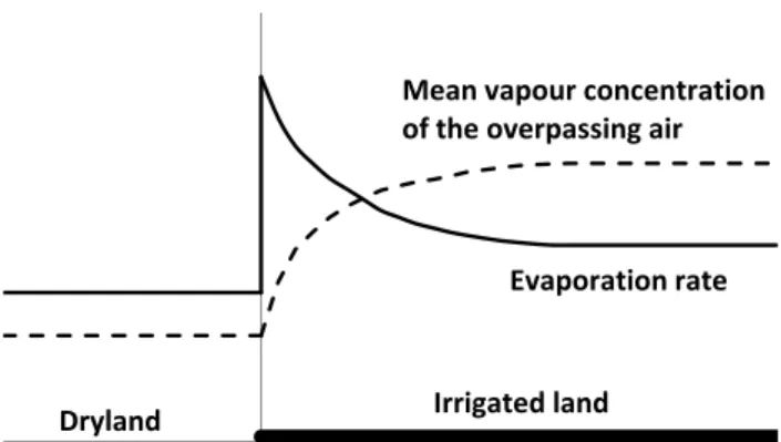
According to Monteith (1965, p. 230), when air moves across a landscape, water vapour is transported at a rate equal to the product of the water vapour content and the wind speed. This transport is known as an advective flow and is present throughout the atmosphere. As shown in Fig. 1, when air moves from a dry region to a wetter area, the con-centration of water vapour increases at the transition to a higher value downwind. On the other hand, at the transi-tion the evaporatransi-tion rate immediately increases to a much higher value compared to that over the dryland, and then de-creases slowly to a value representative of the wetter area. The low evaporation over the dryland means the overpass-ing air will be hotter and drier, thus increasoverpass-ing the available heat energy to increase evaporation in the downwind wetter area (Morton, 1983a, p. 3). In this context, it should be noted that because a lake is defined as one so wide that the effects of an upwind transition (as in Fig. 1) are negligible, overall lake evaporation is independent of the wetness of the upwind environment (Morton, 1983a, p. 17).
Throughout the paper, unless otherwise stated, pan evap-oration means a Class-A evapevap-oration pan with a standard screen. A Class-A evaporation pan, which was developed in the United States and is used widely throughout the world, is a circular pan (1.2 m in diameter and 0.25 m deep) constructed of galvanised iron and is supported on a wooden frame 30 to 50 mm above the ground (WMO, 2006, Sect. 10.3.1). In Australia, a standard wire screen covers the
Dryland Irrigated land
Evaporation rate Mean vapour concentration of the overpassing air
Fig. 1.Conceptual representation of the effect of advected air pass-ing from dryland over an irrigated area.
water surface to prevent water consumption by animals and birds (Jovanovic et al., 2008, Sect. 2).
In this paper, the term “lake” includes lakes, reservoirs and voids (as a result of surface mining) and is defined, following Morton (1983b, p. 84), as a body of water so wide that the ad-vection of air with low water vapour concentration from the adjacent terrestrial environment has negligible effect on the evaporation rate beyond the immediate shoreline or transi-tion zone. Furthermore, Morton distinguishes between shal-low and deep lakes, the former being one in which seasonal heat storage changes are insignificant. Deep lakes may also be considered shallow if one is interested only in annual or mean annual evaporation because at those time steps sea-sonal heat storage changes are considered unimportant (Mor-ton, 1983b, Sect. 3). However, for other procedures there is no clear distinction between shallow and deep lakes (see Ta-ble S5) and, therefore, we have identified them as shallow or deep in terms of the description in the relevant reference.
Because of the scope of evaporation topics across analy-ses and measurements, we deliberately restrict the content of the paper to techniques that can be applied at a daily and/or monthly time step. Under each method we set out the time step that is appropriate. Dealing with shorter time steps, say one hour, is mainly a research issue and is beyond the scope of this paper.
In the literature, there is little consistency in the units for the input data, constants and variables. Here, except for sev-eral special cases, we use a consistent set of units and have adjusted the empirical constants accordingly. The adopted units are: evaporation in mm per unit time, pressure in kPa, wind speed in m s−1 averaged over the unit time, and
ra-diation in MJ m−2 per unit time. Furthermore, we
distin-guish between measurements that are cumulated or averaged over 24 h, denoted as “daily” values, and those that are cu-mulated or measured during day-light hours, designated as “day-time” values (Van Niel et al., 2011).
Evaporation can be expressed as depth per unit time, e.g. mm day−1, or expressed as energy during a day and,
follows that 1 mm day−1of evaporation equals 2.45 MJ m−2
day−1. Furthermore, many evaporation equations described
herein express evaporation in units of mm day−1rather than
the correct unit of kg m−2 day−1. In these cases, the unit conversion is 1000 mm m−1/(ρw = ∼1000 kg m−3), which
equals one and, therefore, the conversion factor from kg m−2
to mm is not included in the equation. We remind readers of this equivalence where the equations are defined in the text.
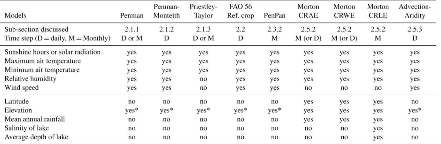
The evaporation models discussed in this paper, including Penman, Penman–Monteith, Priestley–Taylor, reference crop evapotranspiration, PenPan, Morton and advection-aridity models, require a range of meteorological and other data as input. The data required are highlighted in Table 1 along with the time step for analysis and the sections in the paper where the models are discussed. Availability of input data is dis-cussed in Sect. S1. Sections S2 and S3 list the equations for calculating the meteorological variables like saturation vapour pressure, and net radiation. Values of specific con-stants like the latent heat of vaporization, aerodynamic and surface resistances, and albedo values are listed in Tables S1, S2, and S3, respectively.
2 Background theory and models
The evaporation process over a vegetated landscape is linked by two fundamental equations – a water balance equation and an energy balance equation as follows.
Water balance:
P =EAct+Q+1S, (1a)
P = ESoil+ETrans+EInter+Q+1S. (1b)
Energy balance:
R=H+λEAct+G (2)
where, during a specified time period, e.g. one month, and over a given area,P is the mean rainfall (mm day−1),E
Act, ESoil, ETrans, and EInter are respectively the mean actual
evaporation (mm day−1), the mean evaporation from the soil
(mm day−1), the mean transpiration (mm day−1)and mean
evaporation of intercepted precipitation (mm day−1), Qis
the mean runoff (mm day−1),1Sis the change in soil
mois-ture storage (mm day−1)and deep seepage is assumed
neg-ligible,Ris the mean net radiation received at the soil/plant surfaces (MJ m−2day−1),H is the mean sensible heat flux
(MJ m−2 day−1), λE
Act is the outgoing energy (MJ m−2
day−1)as mean actual evaporation,Gis the mean heat con-duction into the soil (MJ m−2day−1), andλis the latent heat of vaporisation (MJ m−2). Models used to estimate
evapora-tion are based on these two fundamental equaevapora-tions.
This section covers five types of models. Section 2.1 (Po-tential evaporation) discusses the conceptual basis for esti-mating potential evaporation, which is followed by Sect. 2.2
(FAO-56 reference crop evapotranspiration) where estimat-ing evapotranspiration for reference crop conditions is con-sidered. Section 2.3 (Pan evaporation) deals with the mea-surement and modelling of evaporation by a Class-A evapo-ration pan. Section 2.4 (Open-surface water evapoevapo-ration) dis-cusses actual evaporation from open-surface water of shal-low lakes, deep lakes (reservoirs) and large voids. Finally, in Sect. 2.5 (Actual evaporation (from catchments)) actual evaporation from landscapes and catchments is discussed. 2.1 Potential evaporation
In 1948, Thornthwaite (1948, p. 56) coined the term “poten-tial evapotranspiration”, the same year that Penman (1948) published his approach for modelling evaporation for a short green crop completely shading the ground. Penman (1956, p. 20) called this “potential transpiration” and since then there have been many definitions and redefinitions of the term potential evaporation or evapotranspiration.
In a detailed review, Granger (1989a, Table 1) (see also Granger, 1989b) examined the concept of potential evapora-tion and identified five definievapora-tions, but considered only three to be useful, which he labelled EP2, EP3 and EP5. They are generally related as
EP5≥EP3≥EP2≥EAct, (3)
where EAct is the actual evaporation rate. EP2, which is
known as the “wet environment” or “equilibrium evapora-tion” rate (see Sect. 2.1.4), is defined as the evaporation rate that would occur from a saturated surface with a constant en-ergy supply to the surface. This represents the lower limit of actual evaporation from a wet surface, noting that for a drier surfaceEAct<EP2. EP2 is effectively the energy flux term in the Penman equation (Eq. 4). EP3 is defined as the evap-oration rate that would occur from a saturated surface with constant energy supply to, and constant atmospheric condi-tions over, the surface. This is equivalent to the Penman evap-oration from a free-water surface and is dependent on avail-able energy and atmospheric conditions. Granger (1989a, Ta-ble 1) denotes EP5 as “potential evaporation” that represents an upper limit of evaporation. It is defined as the evaporation rate that would occur from a saturated surface with constant atmospheric conditions and constantsurfacetemperature.
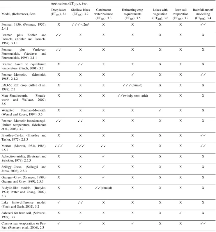
Table 1.Data required to compute evaporation using key models described in the paper.
Penman- Priestley- FAO 56 Morton Morton Morton Advection-Models Penman Monteith Taylor Ref. crop PenPan CRAE CRWE CRLE Aridity
Sub-section discussed 2.1.1 2.1.2 2.1.3 2.2 2.3.2 2.5.2 2.5.2 2.5.2 2.5.3 Time step (D=daily, M=Monthly) D or M D D or M D M M (or D) M (or D) M D Sunshine hours or solar radiation yes yes yes yes yes yes yes yes yes Maximum air temperature yes yes yes yes yes yes yes yes yes Minimum air temperature yes yes yes yes yes yes yes yes yes Relative humidity yes yes no yes yes yes yes yes yes Wind speed yes yes no yes yes no no no yes
Latitude no no no no no yes yes yes no
Elevation yes* yes* yes* yes* yes* yes yes yes yes* Mean annual rainfall no no no no no yes yes yes no Salinity of lake no no no no no no no yes no Average depth of lake no no no no no no no yes no
* To estimate the psychrometric constant.
Reference crop evapotranspiration is the evapotranspiration from a crop with specific characteristics and which is not short of water (Allen et al, 1998, p. 7). Details are given in Sect. 2.2. The second term is actual evaporation, which is defined as the quantity of water that is transferred as wa-ter vapour to the atmosphere from an evaporating surface (Wiesner, 1970, p. 5). Readers are referred to an interesting discussion by Katerji and Rana (2011), who discuss further the definitions of potential evaporation, reference crop evap-otranspiration and evaporative demand.
2.1.1 Penman
In 1948, Penman was the first to combine an aerodynamic approach for estimating potential evaporation with an energy equation based on net incoming radiation. These components of the evaporative process are discussed in Sect. 1.2. This ap-proach eliminates the surface temperature variable, which is not a standard meteorological measurement, resulting in the following equation, known as the Penman or Penman com-bination equation, to estimate potential evaporation (Pen-man, 1948, Eq. 16; see also Shuttleworth, 1992, Sect. 4.2.6; Dingman, 1992, Sect. 7.3.5):
EPen= 1
1+γ
Rn
λ +
γ
1+γEa, (4)
whereEPenis the daily potential evaporation (mm day−1≡
kg m−2day−1)from a saturated surface,R
nis net daily
ra-diation to the evaporating surface (MJ m−2 day−1) where Rn is dependent on the surface albedo (Sect. S3),Ea (mm
day−1)is a function of the average daily wind speed (m s−1), saturation vapour pressure (kPa) and average vapour pres-sure (kPa), 1 is the slope of the vapour pressure curve (kPa◦C−1)at air temperature, γ is the psychrometric
con-stant (kPa◦C−1), and λ is the latent heat of vaporization
(MJ kg−1). E
a is the aerodynamic component in the
Pen-man equation and is discussed in Sect. 2.4.1 and in more de-tail in Sect. S4. The Penman equation assumes no heat ex-change with the ground, no ex-change in heat storage, and no water-advected energy (as inflow in the case of a lake) (Ding-man, 1992, Sect. 7.3.5). Penman (1956, p. 18) and Monteith (1981, p. 4 and 5) provide helpful discussions of the depen-dence of latent heat flux on surface temperature. Application of the Penman equation is discussed in Sect. 2.4.1 with fur-ther details provided in Sect. S4.
The Penman approach has spawned many other proce-dures (e.g. Priestley and Taylor, 1972; see Sect. 2.1.3) in-cluding the incorporation of resistance factors that extend the general method to vegetated surfaces. The Penman–Monteith formulation described in the following section is an example of the latter.
2.1.2 Penman–Monteith
The Penman–Monteith model, defined as Eq. (5), is usually adopted to estimate potential evaporation from a vegetated surface. The fundamental Penman–Monteith formulation de-pends on the unknown temperature of the evaporating sur-face (Raupach, 2001, p. 1154). Raupach provides a detailed discussion of the approaches to eliminate the surface temper-ature from the surface energy balance equations. The sim-plest solution results in the following well known Penman– Monteith equation (Allen et al., 1998, Eq. 3):
ETPM=
1
λ
1(Rn−G)+ρaca(ν
∗
a−νa) ra
1+γ1+rs ra
, (5)
where ETPM is the Penman–Monteith potential evaporation
(mm day−1 ≡kg m−2day−1),R
nis the net daily radiation
at the vegetated surface (MJ m−2day−1),Gis the soil heat
flux (MJ m−2 day−1), ρ
a is the mean air density at
con-stant pressure (kg m−3), c
(MJ kg−1◦C−1),r
a is an “aerodynamic or atmospheric
re-sistance” to water vapour transport (s m−1)for neutral
con-ditions of stability (Allen et al., 1998, p. 20),rs is a “sur-face resistance” term (s m−1), (νa∗−νa)is the vapour
pres-sure deficit (kPa),λ is the latent heat of vaporization (MJ kg−1),1is the slope of the saturation vapour pressure curve
(kPa◦C−1) at air temperature, and γ is the
psychromet-ric constant (kPa◦C−1). Values of r
a and rs are discussed
in Sect. S5. The major difference between the Penman– Monteith and the Penman equations is the incorporation of the two resistance (atmospheric and surface, as described in Sect. 1.2) terms in Penman–Monteith rather than using a wind function. Although the original Penman equation (Pen-man, 1948, Eq. 16) does not include a soil heat flux term, Penman noted that for his test chamber the heat conducted through the walls of the container was negligible.
2.1.3 Priestley–Taylor
The Priestley–Taylor equation (Priestley and Taylor, 1972, Eq. 14) allows potential evaporation to be computed in terms of energy fluxes without an aerodynamic component as follows
EPT=αPT
1
1+γ
Rn
λ −
G λ
, (6)
where EPTis the Priestley–Taylor potential evaporation (mm
day−1≡kg m−2day−1),R
nis the net daily radiation at the
evaporating surface (MJ m−2day−1),Gis the soil flux into
the ground (MJ m−2 day−1),1is the slope of the vapour
pressure curve (kPa◦C−1)at air temperature,γ is the
psy-chrometric constant (kPa◦C−1), andλis the latent heat of
vaporization (MJ kg−1).α
PTis the Priestley–Taylor constant.
Based on non-water-limited field data, Priestley and Tay-lor (1972, Sect. 6) adoptedαPT=1.26 for “advection-free”
saturated surfaces. Eichinger et al. (1996, p. 163) developed an analytical expression forαPTand found that 1.26 was an appropriate value for an irrigated bare soil. Lhomme (1997) developed a theoretical basis for the Priestley–Taylor coef-ficient of 1.26 for non-advective conditions. Based on field data in northern Spain, Castellvi et al. (2001) found thatαPT
exhibited large seasonal (up to 27 %) and spatial (αPT=1.35
to 1.67) variations. Improved performance was achieved by including adjustments for vapour pressure deficit and avail-able energy. Pereira (2004), noting the analysis by Mon-teith (1965, p. 220) and Perrier (1975), considered the hy-pothesisαPT=−1whereis a decoupling coefficient and
is a function of the aerodynamic and surface resistances, im-plyingαPT is not a constant. The decoupling coefficient is
discussed in Sect. S5. Values ofαPTfor a range of surfaces
are listed in Table S8 and it is noted thatαPTvalues are
de-pendent on the observation period, daily (24 h) or day-time. Priestley and Taylor (1972, Sect. 1) adopted a daily time step for their analysis.
2.1.4 Equilibrium evaporation
Slatyer and McIlroy (1961) developed the concept of equilib-rium evaporation (EEQ)in which air passing over a saturated
surface will gradually become saturated until an equilibrium rate of evaporation is attained. Edinger et al. (1968) defined equilibrium temperature as the surface temperature of the evaporating surface at which the net rate of heat exchange (by shortwave and longwave radiation, conduction and evapora-tion) is zero. But because of the daily cycles in the meteoro-logical conditions, equilibrium temperature is never achieved (Sweers, 1976, p. 377).
Stewart and Rouse (1976, Eq. 4) interpreted the Slatyer and McIlroy (1961) concept in terms of the Priestley and Taylor (1972) equation as
EEQ=
1
αPT
EPT, (7)
whereEPT andαPTare defined in the previous section.
Mc-Naughton (1976) proposed a similar argument. However, based on lysimeter data Eichinger et al. (1996) question this concept of equilibrium evaporation and suggest that the Priestley–Taylor equation withαPT=1.26 is more
represen-tative of equilibrium evaporation under wet surface condi-tions. In 2001, Raupach (2001) carried out a historical review and theoretical analysis of the concept of equilibrium evapo-ration. He concluded that for any closed evaporating system (that is, a system in which there is no mass exchange with the external environment theoretically approximated by a large area with an inversion, provided entrainment is small) with steady energy supply, the system moves towards a quasi-steady state in which the Bowen ratio (β) takes the equi-librium value of 1/ε, whereε is the ratio of latent to sen-sible heat contents of saturated air in a closed system. Rau-pach (2001) also concluded that open systems cannot reach equilibrium.
2.1.5 Other methods for estimating potential evaporation
There are many other potential evaporation equations pro-posed and evaluated during the past 100 or so years that could have been included in this paper. Some of these, e.g. Thornth-waite (ThornthThornth-waite, 1948) and Makkink models (Keijman, 1981, p. 22; de Bruin, 1987, footnote p. 19), are discussed in Sect. S9.
2.2 FAO-56 reference crop evapotranspiration
Adopting the characteristics of a hypothetical reference crop (height=0.12 m, surface resistance=70 s m−1, and albedo
(Food and Agriculture Organization) FAO-56 reference crop or the standardized reference evapotranspiration equation, short (ASCE, 2005, Table 1), and is defined as follows
ETRC=
0.4081(Rn−G)+γTa900+273u2(ν ∗ a−νa) 1+γ (1+0.34u2)
, (8)
where ETRC is the daily reference crop evapotranspiration
(mm day−1≡kg m−2day−1),T
ais the mean daily air
tem-perature (◦C) at 2 m, andu
2is the average daily wind speed
(m s−1) at 2 m. Other symbols are as defined previously.
Allen et al. (1998) provide a detailed explanation of the de-velopment of Eq. (8) from Eq. (5) including an explanation of the units of 0.408 (kg MJ−1), 900 (kg m−3s day−1)and 0.34
(s m−1). A detailed explanation of the theory of reference
crop evapotranspiration is presented by McVicar et al. (2005, Sect. 2). It should be noted that a second reference crop evap-otranspiration equation has been developed for a 0.5 m tall crop (ASCE, 2005, Table 1). Further details are included in Sect. S5.
The time step recommended by Allen et al. (1998, Chap-ter 4) for analysis using Eq. (8) is one day (24 h). Equations for other time steps may be found in the same reference.
A detailed discussion of the variables is given in Sect. S5.
Gis a function of successive daily temperatures and, there-fore, ETPMand ETRCare sensitive toGwhen there is a large
difference between successive daily temperatures. An algo-rithm for estimatingGis presented in Sect. S5. It should be noted that the Penman–Monteith equation assumes that the actual evaporation does not affect the overpassing air (Wang et al., 2001).
There are other equations for estimating reference crop evapotranspiration, e.g. FAO-24 Blaney and Criddle (Allen and Pruitt, 1986), Turc (1961), Hargreaves–Samani (Harg-reaves and Samani, 1985), and the modified Harg(Harg-reaves ap-proach (Droogers and Allen, 2002). These are included in Sect. S9.
2.3 Pan evaporation
2.3.1 Class-A evaporation pan
Evaporation data from a Class-A pan, when combined with an appropriate pan coefficient or with an adjustment for the energy exchange through the sides and bottom of the tank, can be considered to be open-water evaporation (Dingman, 1992, p. 289). Pan data can be used to estimate actual evap-oration for situations that require free-water evapevap-oration as follows
Efw,j=KjEPan,j, (9)
where Efw,j is an estimate of monthly (or daily)
open-surface water evaporation (mm/unit time),j is the specific month (or day),Kj is the average monthly (or daily)
Class-A pan coefficient, andEPan,j is the monthly (or daily)
ob-served Class-A pan value (mm/unit time). Usually, pan co-efficients are estimated by comparing observed pan evapo-rations with estimated or measured open-surface water esti-mates, although Kohler et al. (1955) and Allen et al. (1998, p. 86) proposed empirically derived relationships. These are described in Sect. S16. Published pan coefficients are avail-able for a range of regions and countries. Some of these are reported also in Sect. S16 and associated tables. In addition, monthly Class-A pan coefficients are provided for 68 loca-tions across Australia (Sect. S16 and Table S6). In China, micro-pans (200 mm diameter, 100 mm high that are filled to 20 or 30 mm) are used to measure pan evaporation. Based on an analytical analysis of the pan energetics (McVicar et al., 2007b, p. 209), the pan coefficients for a Chinese micro-pan are lower than Class-A pan coefficients but with a seasonal range being similar to those of a Class-A pan.
Masoner et al. (2008) compared the evaporation rate from a floating evaporation pan (which estimated open-surface water evaporation – see Keijman and Koopmans, 1973; Ham and DeSutter, 1999) with the rate from a land-based Class-A pan. They concluded that the floating pan to land pan ratios were similar to Class-A pan coefficients used in the United States.
The disaggregation of an annual actual or potential evapo-ration estimate into monthly or especially daily values is not straightforward, assuming there is no concurrent at-site cli-mate data which could be used to gain insight into how the annual value should be partitioned. One approach is to use monthly pan coefficients if available, as noted above. An-other approach, that is available to Australian analysts, is to adopt average monthly values of point potential evapotran-spiration for the given location (maps for each month are pro-vided in Wang et al., 2001) and pro rata the values to sum to the annual values ofEfw. This suggestion is based on the
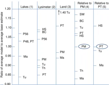
re-cent analysis by Kirono et al. (2009, Fig. 3) who found that, for 28 locations around Australia, Morton’s potential evap-otranspiration ETPot (see Sect. 2.5.2) correlated
satisfacto-rily (R2= 0.81) with monthly Class-A pan evaporation ues, although the Morton values overestimated the pan val-ues by approximately 11 %. Further discussion is provided in Sect. 3.1.3.
2.3.2 The PenPan model
can successfully estimate monthly and annual Class-A pan evaporation at sites across Australia.
Following Rotstayn et al. (2006, Eq. 2) the PenPan equa-tion is defined as
EPenPan= 1 1+apγ
RNPan
λ +
apγ
1+apγfPan(u)(ν
∗
a−νa)
, (10)
where EPenPan is the modelled Class-A (unscreened) pan
evaporation (mm day−1≡kg m−2day−1),R
NPanis the net
daily radiation at the pan (MJ m−2day−1),1is the slope of
the vapour pressure curve (kPa◦C−1)at air temperature,γis
psychrometric constant (kPa◦C−1), andλis the latent heat
of vaporization (MJ kg−1),a
p is a constant adopted as 2.4
(Rotstayn et al., 2006, p. 2),νa∗−νais vapour pressure deficit
(kPa), andfPan(u)is defined as (Thom et al., 1981, Eq. 34)
fPan(u)=1.202+1.621u2, (11)
where u2 is the average daily wind speed at 2 m height
(m s−1). Details to estimateR
NPanand results of the
applica-tion of the model to 68 Australian sites are given in Sect. S6. 2.4 Open-surface water evaporation
In this paper the terms open-water evaporation and free-water evaporation are used interchangeably and assume that wa-ter available for evaporation is unlimited. We discuss two approaches to estimate open-water evaporation: Penman’s combination equation and an aerodynamic approach. 2.4.1 Penman equation
The Penman equation (Penman, 1948, Eq. 16) is widely and successfully used for estimating open-water evaporation as
EPenOW=
1
1+γ
Rnw
λ +
γ
1+γEa, (12)
whereEPenOW is the daily open-surface water evaporation
(mm day−1≡kg m−2day−1),R
nwis the net daily radiation
at the water surface (MJ m−2day−1), and other terms have
been previously defined. In estimating the net radiation at the water surface, the albedo value for water should be used (Table S3). Details of the Penman calculations are presented in Sect. S4. Section S3 lists the equations required to com-pute net radiation with or without incoming solar radiation measurements. We note that of the 20 methods reviewed by Irmak et al. (2011) the method described in Sect. S3 (based on Allen et al. (1998, p. 41 to 55)) to estimateRnwwas one of the better performing procedures.
The first term in Eq. (12) is the radiative component and the second term is the aerodynamic component. To estimate
Rnw, the incoming solar radiation (Rs), measured at
auto-matic weather stations or estimated from extraterrestrial radi-ation, is reduced by estimates of shortwave reflection, using the albedo for water, and net outgoing longwave radiation.Ea
is known as the aerodynamic equation (Kohler and Parmele, 1967, p. 998) and represents the evaporative component due to turbulent transport of water vapour by an eddy diffusion process (Penman, 1948, Eq. 1) and is defined as
Ea=f (u)(νa∗−νa) , (13)
wheref (u)is a wind function typically of the formf (u)=
a+bu, and ν∗a−νais the vapour pressure deficit (kPa).
There have been many studies dealing with Penman’s wind function including Penman’s (1948, 1956) analyses (see Penman (1956, Eq. 8a and b) for a comparison of the two equations), Stigter (1980, p. 322, 323), Fleming et al. (1989, Sect. 8.4), Linacre (1993, Appendix 1), Cohen et al. (2002, Sect. 4) and Valiantzas (2006). Based on Valiantzas’ (2006, page 695) summary of these studies, we recommend that the Penman (1956, Eq. 8b) wind function be adopted as the standard for evaporation from open water witha=1.313 andb=1.381 (wind speed is a daily average value in m s−1 and the vapour deficit in kPa). Typically, the wind function assumes wind speed is measured at 2 m above the ground surface but if not it should be adjusted using Eq. (S4.4). More details about alternative wind functions are provided in Sect. S4. It is noted here that because the wind function coefficients were empirically derived, the Penman equation for a specific application is an empirical one.
According to Dingman (1992, p. 286), in the Penman equation it is assumed there is no change in heat storage, no heat exchange with the ground, and no advected energy. Data required to use the equation include solar radiation, sunshine hours or cloudiness, wind speed, air temperature, and relative humidity (or dew point temperature). Although Penman (1948) carried out his computations of evaporation based on 6-day and monthly time steps, most analysts have adopted a monthly time step (e.g. Weeks, 1982; Fleming et al., 1989, Sect. 8.4; Chiew et al., 1995; Cohen et al., 2002; Harmsen et al., 2003) and several have used a daily or shorter time step (e.g. Chiew et al., 1995; Sumner and Jacobs, 2005). van Bavel (1966) amended the original Penman (1948) equation to take into account boundary layer resistance. The modified equation is considered in Sect. S4.
Linacre (1993, p. 239) discusses potential errors in the Penman equation and the accuracy of the estimates, and re-ports that lake evaporation estimates are much more sensitive to errors in net radiation and humidity than to errors in air temperature and wind.
2.4.2 Aerodynamic formula
relationship to estimate open surface water evaporation.
ELarea=(2.36+1.67u2)A−0.05(νa∗−νa), (14)
whereELarea is an estimate of open-surface water evapora-tion (mm day−1)as a function of evaporating area,A, (m2),
u2is the wind speed (m s−1)over land at 2 m height,νw∗ is
the saturated vapour pressure (kPa) at thewater surface, and
νais the vapour pressure (kPa) at air temperature.
2.5 Actual evaporation (from catchments)
2.5.1 The complementary relationship
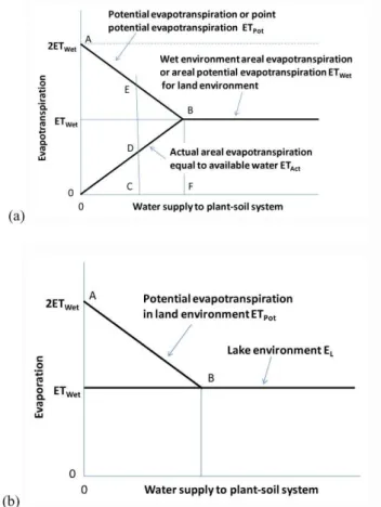
In 1963, Bouchet hypothesised that, for large homogeneous areas where there is little advective heat and moisture (dis-cussed in Sect. 1.2), potential and actual evapotranspira-tion depend on each other in a complementary way via feedbacks between the land and the atmosphere. This led Bouchet (1963) to propose the complementary relationship (CR) illustrated in Fig. 2 and defined as
ETAct=2ETWet−ETPot. (15)
ETActis the actual areal or regional evapotranspiration (mm
per unit time) from an area large enough that the heat and vapour fluxes are controlled by the evaporating power of the lower atmosphere and unaffected by upwind transitions (In the context of the complementary relationship, and tech-niques using the relationship, ETAct includes transpiration
and evaporation from water bodies, soil and interception stor-age). ETWetis the potential (or wet-environment)
evapotran-spiration (mm per unit time) that would occur under steady state meteorological conditions in which the soil/plant sur-faces are saturated and there is an abundant water supply. Ac-cording to Morton (1983a, p. 16), ETWetis equivalent to the
conventional definition of potential evapotranspiration. ETPot
is the (point) potential evapotranspiration (mm per unit time) for an area so small that the heat and water vapour fluxes have no effect on the overpassing air, in other words, evaporation that would occur under the prevailing atmospheric conditions if only the available energy were the limiting factor.
Consider an infinitesimal point in an arid landscape with no soil moisture (origin of Fig. 2a). We observe from the CR (Eq. 15) that actual areal evapotranspiration ETAct=0
and, therefore, ETPot=2ETWet. For the same location and
the same evaporative energy, when the soil becomes wet af-ter rainfall actual evapotranspiration can take place. Consider point C in Fig. 2. The actual areal evapotranspiration has increased to D with a corresponding decrease in point po-tential evapotranspiration as modelled by the CR (Eq. 15). However, when the landscape becomes saturated (point F in Fig. 2a), that is, the water supply to the plants is not limiting, ETAct=ETPot=ETWet.
The complementary relationship is the basis for esti-mating actual and potential evapotranspiration by the three
Morton (1983a) models (known as Complementary Re-lationship Areal Evapotranspiration (CRAE), Complemen-tary Relationship Wet-surface Evaporation (CRWE) and Complementary Relationship Lake Evaporation (CRLE)) and by the Advection-Aridity (AA) model of Brutsaert and Strickler (1979) with modifications by Hobbins et al. (2001a, b).
In his 1983a paper, Morton argues that the CR cannot be verified directly, but based on a water balance study of four rivers in Malawi and another in Puerto Rico, he argued that the concept is plausible (Morton, 1983a, Figs. 7–9). Based on independent evidence of regional ETActand on pan
evap-oration data from 192 observations in 25 catchments in the US, Hobbins and Ram´ırez (2004) and Ram´ırez et al. (2005) argue that the complementary relationship is beyond con-jecture. The shape of the CR relationship for the observed pan data, assuming a pan represents an infinitesimal point as required in the CR relationship, is similar to the shape in Fig. 2a. Using a mesoscale model over an irrigation area in south-eastern Turkey, Ozdogan et al. (2006) concluded that their results lend credibility to the CR hypothesis. However, research is underway into understanding whether the con-stant of proportionality (“2” in Eq. 15) varies and, if so, what is the nature of the asymmetry in the relationship (Ram´ırez et al., 2005; Szilagyi, 2007; Szilagyi and Jozsa, 2008). Some other references of relevance include Hobbins et al. (2001a); Yang et al. (2006); Kahler and Brutsaert (2006); Lhomme and Guilioni (2006); Yu et al. (2009) and Han et al. (2011). 2.5.2 Morton’s models
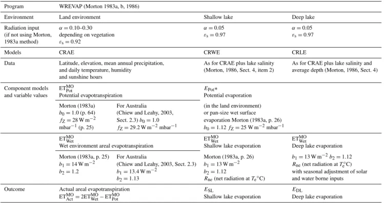
Table 2.Morton’s models (αis albedo,εsis surface emissivity, andb0,b1,b2andfZare defined in Sect. S7).
Program WREVAP (Morton 1983a, b, 1986)
Environment Land environment Shallow lake Deep lake
Radiation input α=0.10–0.30 α=0.05 α=0.05
(if not using Morton, depending on vegetation εs=0.97 εs=0.97
1983a method) εs=0.92
Models CRAE CRWE CRLE
Data Latitude, elevation, mean annual precipitation, As for CRAE plus lake salinity As for CRAE plus lake salinity and and daily temperature, humidity (Morton, 1986, Sect. 4, item 2) average depth (Morton, 1986, Sect. 4) and sunshine hours
Component models ETMOPot EPot∗
and variable values Potential evapotranspiration Potential evaporation
Morton (1983a) For Australia (in the land environment)
b0=1.0 (p. 64) (Chiew and Leahy, 2003, or pan-size wet surface
fZ=28 W m−2 Sect. 2.3)b0=1.0 evaporation Morton (1983a, p. 26)
mbar−1(p. 25) fZ=29.2 W m−2mbar−1 b0=1.12fZ=25 W m−2mbar−1
ETMOWet ETMOWet ETMOWet
Wet environment areal evapotranspiration Shallow lake evaporation Deep lake evaporation
Morton (1983a, p. 25) For Australia Morton (1983a, p. 26) b1=13 W m−2b2=1.12
b1=14 W m−2 (Chiew and Leahy, 2003, Sect. 2.3) b1=13 W m−2 Rne(net radiation atTe◦C)
b2=1.2 b1=13.4 W m−2 b2=1.12 with seasonal adjustment of solar
b2=1.13 Rne(net radiation atTe◦C) and water borne inputs
Outcome Actual areal evapotranspiration ESL EDL
ETMO
Act=2ETMOWet−ETMOPot Shallow lake evaporation Deep lake evaporation
* According to Morton (1986, p. 379, item 4) in the context of estimating lake evaporation,EPothas no “. . . real world meaning. . . ” because the estimates are sensitive to both the lake energy environment and the land temperature and humidity environment which are significantly out of phase. This is not so with lake evaporation as the model accounts for the impact of overpassing air.
CRAE model
The CRAE model estimates the three components: poten-tial evapotranspiration, wet-environment areal evapotranspi-ration and actual areal evapotranspievapotranspi-ration.
Estimating potential evapotranspiration (ETPotin Fig. 2).
Because Morton’s (1983a, p. 15) model does not require wind data, it has been used extensively in Australia (where historical wind data were unavailable until recently; see McVicar et al., 2008) to compute time series estimates of his-torical potential evaporation. Morton’s approach is to solve the following energy-balance and vapour transfer equations respectively for potential evaporation at the equilibrium tem-perature, which is the temperature of the evaporating surface:
ETMOPot = 1
λ n
Rn− [γpfv+4ǫsσ (Te+273)3](Te−Ta)
o
, (16)
ETMOPot =1
λ
fv(νe∗−ν ∗
D) , (17)
where ETMOPot is Morton’s estimate of potential evapotran-spiration (mm day−1≡kg m−2 day−1),R
n is net radiation
for soil/plant surfaces at air temperature (W m−2),f vis the
vapour transfer coefficient (W m−2mbar−1)and is a function
of atmospheric stability (details are provided in Sect. S7 or Morton (1983a, p. 24–25)),εsis the surface emissivity,σ is
the Stefan–Boltzmann constant (W m−2K−4),T
eandTaare
the equilibrium temperature (◦C) and air temperature (◦C)
re-spectively,νe∗is saturation vapour pressure (mbar) atTe,νD∗
is the saturation vapour pressure (mbar) at dew point temper-ature,λis the latent heat of vaporisation (W day kg−1)and γpis a constant (mbar◦C−1). Solving for ET
Pot andTe is
an iterative process and guidelines are given in Sect. S7. A worked example is provided in Sect. S21.
Estimating wet-environment areal evapotranspiration (ETWetin Fig. 2).
Morton (1983b, p. 79) notes that the wet-environment areal evapotranspiration is the same as the conventional definition of potential evapotranspiration. To estimate the wet-environment areal evapotranspiration, Morton (1983a, Eq. 14) added a term (b1)to the Priestley–Taylor equation
(see Sect. 2.1.3 for a discussion of Priestley–Taylor) to ac-count for atmospheric advection as follows
ETMOWet=1
λ
b1+b2
Rne
1+γp1
e
, (18)
where ETMOWet is the wet-environment areal evapotranspira-tion (mm day−1),R
Fig. 2. Theoretical form of the complementary relationship for:
(a)land environment and(b)lake environment (adapted from Mor-ton, 1983a, Figs. 5 and 6). In Fig. 2a, at point B and beyond where there is adequate water supply (saturated soil moisture), actual evap-otranspiration equals areal potential evapevap-otranspiration. As the wa-ter supply reduces below B, evaporative energy not used in ac-tual evapotranspiration remains as potential evapotranspiration as required by the complementary relationship (i.e. ETAct= 2ETWet
-ETPot).
soil/plant surface at the equilibrium temperatureTe(◦C),γ
is the psychrometric constant (mbar◦C−1),pis atmospheric
pressure (mbar),1e is slope of the saturation vapour
pres-sure curve (mbar◦C−1)at T
e, b1 (W m−2)andb2 are the
empirical coefficients, and the other symbols are as defined previously. Details to estimateRneare given in Sect. S7.
Estimating (actual) areal evapotranspiration (ETActin Fig. 2).
Morton (1983a) formulated the CRAE model to estimate ac-tual areal evapotranspiration (ETMOAct)(mm day−1)from the
complementary relationship (Eq. 15) as follows
ETMOAct =2ETMOWet−ETMOPot , (19) ETMOPot and ETMOWetare estimated from Eqs. (16) and (17), and Eq. (18) respectively.
In the Morton (1983a) paper (Fig. 13), Morton com-pared estimates of actual areal evapotranspiration with water-budget estimates for 143 river basins worldwide and found the monthly estimates to be realistic. Others have assessed various parts of the CRAE model. Based on a study of 120 minimally impacted basins in the US, Hobbins et al. (2001a, p. 1378) found that the CRAE model overestimated annual evapotranspiration by only 2.5 % of the mean annual precip-itation with 90 % of values being within 5 % of the water balance closure estimate of actual evapotranspiration. Szi-lagyi (2001), inter alia, checked how well WREVAP (incor-porating the CRAE program) estimated values of incident global radiation at 210 sites and estimates of pan evaporation at 19 stations with measured values. The respective correla-tions were 0.79 (Fig. 3 of Szilagyi, 2001) and 0.87 (Fig. 4 of Szilagyi, 2001).
For application of the CRAE model accurate estimates of air temperature and relative humidity are required from a rep-resentative land-based location (Morton, 1986, p. 378). For CRAE, Morton (1983a, p. 28) suggested a 5-day limit as the minimum time step for analysis.
CRWE model
In Morton’s (1983a) paper, he formulated and documented the CRAE model for land surfaces. In a second paper, Mor-ton (1983b) converts CRAE to a complementary relation-ship lake evaporation which he designated as CRLE. How-ever, in 1986 Morton (1986) introduced the complementary relationship wet-surface evaporation known as the CRWE model to estimate “lake-size wet surface evaporation” (Mor-ton, 1986, p. 371), in other words, evaporation from shallow lakes. The evaporation from a shallow lake differs from the wet-environment areal evapotranspiration because the radia-tion absorpradia-tion and vapour pressure characteristics between water and land surfaces are different (Morton, 1983b, p. 80) as documented in Table 2. It should also be noted that, for a lake, potential evaporation and actual evaporation will be equal but, for a land surface, actual evaporation will be less than potential evaporation, except when the surface is satu-rated (Morton, 1986, p. 81). Normally, land-based meteoro-logical data would be used (Morton, 1983a, p. 70) but data measured over water has only a “relatively minor effect” on the estimate of lake evaporation (Morton, 1983b, p. 96).
In the 1983b paper, Morton (1983b, Eq. 11) introduced an equation (Eq. 23 herein) to deal with estimating evaporation from small lakes, farm dams and ponds.
CRLE model
evaporation (Morton, 1983b, p. 84) and the CRWE formu-lation would be used. Over an annual cycle there is no net change in the heat storage, although there is a phase shift in the seasonal evaporation, so that the sum of the seasonal lake evaporation approximately equals the annual estimate.
Morton’s (1983b, Sect. 3) paper provides, inter alia, a rout-ing technique which takes into account the effect of depth, salinity and seasonal heat changes on monthly lake evapo-ration. This is only approximate as seasonal heat changes in a lake should be based on the vertical temperature pro-files which rarely will be available. In 1986, Morton changed the form of the routing algorithm outlined in Morton (1983b, Sect. 3) to a classical linear storage routing model (Morton, 1986, p. 376). This is the one we have adopted in the For-tran 90 listing of WREVAP (Sect. S20) and in the WREVAP worked example (Sect. S21).
Morton (1979, 1983b) validated his approach for estimat-ing lake evaporation against water budget estimates for ten major lakes in North America and East Africa. The aver-age absolute percentaver-age deviation between the model of lake evaporation and water budget estimates was 3.7 % of the wa-ter budget estimates (Morton, 1979, p. 72).
Morton (1986, p. 378) notes that, because the complemen-tary relationship takes into account the differences in sur-rounding, for the CRLE model it matters little where the meteorological measurements are made in relation to the lake; they can be land-based or from a floating raft.
Because routing of solar and water-borne energy is incor-porated in the CRLE model, a monthly time step is adopted (Morton, 1983b, Sect. 9). Land-based meteorological data would normally be used (Morton, 1983b, p. 82) but as noted above data measured over water has only a minor effect on the estimate of lake evaporation (Morton, 1983b, p. 96; 1986, p. 378). Details of the application of Morton’s procedures for estimating evaporation from a shallow lake, farm dam or deep lake are discussed in Sect. S7.
A worked example applying program WREVAP using a monthly time step is found in Sect. S21.
2.5.3 Advection-aridity and like models
Based on the complementary relationship (Eq. 15), Brut-saert and Strickler (1979, p. 445) proposed the original advection-aridity (AA) model in which they adopted the Pen-man equation (Eq. 4) for the potential evapotranspiration (ETPot)and the Priestley–Taylor equation (Eq. 6) for the
wet-environment evapotranspiration (ETWet) to estimate actual
evaporation as follows
EBSAct=(2αPT−1) 1 1+γ
Rn
λ − γ
1+γf (u2)(ν
∗
a−νa)
, (20)
where EActBS is the actual evapotranspiration estimated by the Brutsaert and Strickler equation (mm day−1≡kg m−2
day−1),α
PTis the Priestley–Taylor coefficient, and the other
symbols are as defined previously. In their analysis Brutsaert and Strickler (1979, Abstract) adopted a daily time step.
In a study of 120 minimally impacted basins in the United States, Hobbins et al. (2001a, Table 2) found that the Brut-saert and Strickler (1979) model underestimated actual an-nual evapotranspiration by 7.9 % of mean anan-nual precipi-tation, and for the same basins, Morton’s (1983a) CRAE model overestimated actual annual evapotranspiration by only 2.4 % of mean annual precipitation. Several modifica-tions to the original AA model have been put forward. Hob-bins et al. (2001b) reparameterized the wind functionf (u2)
on a monthly regional basis and recalibrated the Priestley– Taylor coefficient yielding small differences between com-puted evapotranspiration and water balance estimates. How-ever, the regional nature of the wind function restricts the recalibrated model to the conterminous United States.
Alternatives to the advection-aridity model of Brutsaert and Strickler (1979) are the approach by Szilagyi (2007), amended by Szilagyi and Jozsa (2008); the Granger model (Granger, 1989b; Granger and Gray, 1989), which is not based on the complementary relationship; and the Han et al. (2011) modification of the Granger model. Details are presented in Sect. S8.
3 Practical topics in estimating evaporation
To address the practical issue of estimating evaporation one needs to keep in mind the setting of the evaporating surface along with the availability of meteorological data. The set-ting is characterised by several features: the meteorological conditions in which the evaporation is taking place, the water available for evaporation, the energy stored within the evapo-rating body, the advected energy due to water inputs and out-puts from the evaporating water body, and the atmospheric advected energy.
upwind fringe of the area but the bulk of the area will experi-ence a moisture-laden environment. On the other hand, for a small lake or farm dam, a small irrigation area or an irrigation canal in a dry region, the associated atmosphere will be min-imally affected by the water body and the prevailing upwind atmosphere will be the driving influence on the evaporation rate.
In the following discussion, we assume that: (i) at-site daily meteorological data from an automatic weather sta-tion (AWS) are available; or (ii) meteorological data mea-sured manually at the site and at an appropriate time interval are available; or (iii) at-site daily pan evaporation data are available. At some AWSs, hard-wired Penman or Penman– Monteith evaporation estimates are also available. Methods to estimate evaporation where meteorological data are not available are discussed in Sect. 4.3.
When incorporating estimates of lake evaporation into a water balance analysis of a reservoir and its related catch-ment, it is important to note that double counting will occur if the inflows to the reservoir are based on the catchment area including the inundated area and then an adjustment is made to the water balance by adding rainfall to and subtracting lake evaporation from the inundated area. The correct adjustment is the difference between evaporation prior to inundation and lake evaporation (see McMahon and Adeloye, 2005, p. 97 for a fuller explanation of this potential error).
3.1 Deep lakes
This paper does not address the measurement of tion from lakes but rather the estimation of lake evapora-tion by modelling. A helpful review article on the measure-ment and the calculation of lake evaporation is by Finch and Calver (2008).
In dealing with deep lakes (including constructed stor-ages, reservoirs and large voids), three issues need to be ad-dressed. First, the heat storage of the water body affects the surface energy flux and, because the depth of mixing varies in space and time and is rarely known, it is difficult to estimate changes at a short time step; typically, a monthly time step is adopted. Second, the effects of water advected energy needs to be considered. If the inflows to a lake are equivalent to a large depth of the lake area and their average temperatures are significantly different, advected energy needs to be taken into account (Morton, 1979, p. 75). Third, increased salinity reduces evaporation and, therefore, changes in lake salinity need to be addressed. Next, we explore three procedures for estimating evaporation from deep lakes.
3.1.1 Penman model
To estimate evaporation from a deep lake, the Penman esti-mate of evaporation,EPenOW, (Eq. 12) is a starting point.
Wa-ter advected energy (precipitation, streamflow and ground-water flow into the lake) and heat storage in the lake
are accounted for by the following equation recommended by Kohler and Parmele (1967, Eq. 12) and reported by Dingman (1992, Eqs. 7–37) as
EDL=EPenOW+αKP
Aw− 1Q
1t
, (21)
where EDL is the evaporation from the deep lake (mm
day−1),E
PenOWis the Penman or open-surface water
evapo-ration (mm day−1),α
KPis the proportion of the net addition
of energy from water advection and storage used in evapora-tion during1t,Aw is the net water advected energy during 1t (mm day−1), and 1Q
1t is the change in stored energy
ex-pressed as a water depth equivalent (mm day−1). The latter
three terms are complex and are set out in Sect. S10 along with details of the procedure.
Vardavas and Fountoulakis (1996, Fig. 4), using the Pen-man model, estimated the monthly lake evaporation for four reservoirs in Australia and found the predictions agreed sat-isfactorily with mean monthly evaporation measurements. Change in heat storage is based on the monthly surface water temperatures. Thus:
EDL= 1
1+γ
R
n+1H
λ
+ γ
1+γEa, (22)
where EDL is the evaporation from the deep lake (mm
day−1≡kg m−2day−1),R
n is the net radiation at the
wa-ter surface (MJ m−2 day−1), E
a is the evaporation
com-ponent (mm day−1) due to wind, 1 is the slope of the
vapour pressure curve (kPa ◦C−1) at air temperature, γ
is the psychrometric constant (kPa ◦C−1), λ is the latent heat of vaporization (MJ kg−1), and 1H is the change in heat storage (MJ m−2 day−1). We detail the Vardavas and
Fountoulakis (1996) method in Sect. S10. 3.1.2 Morton evaporation
In Morton’s WREVAP program, monthly evaporation from deep and shallow lakes can be estimated. As noted in Sect. 2.5.2, for annual evaporation estimates, there is no dif-ference in magnitude between deep and shallow lake evapo-ration (see also Sacks et al., 1994, p. 331). In Morton’s pro-cedure, seasonal heat changes in deep lakes are incorporated through linear routing. Details are presented in Sect. S7. The data for Morton’s WREVAP program are mean monthly air temperature, mean dew point temperature (or mean monthly relative humidity) and monthly sunshine hours as well as lat-itude, elevation and mean annual precipitation at the site. The broad computational steps are set out in Sect. S7 and details can be found in Appendix C of Morton (1983a). A Fortran 90 listing of a slightly modified version of the Morton WRE-VAP program is provided in Sect. S20 and a worked example is available in Sect. S21.
used to estimate lake evaporation directly. Comparing CRLE lake evaporation estimates with water budgets for 17 lakes worldwide, Morton (1986, p. 385) found the annual estimates to be within 7 %. In a lake study in Brazil, dos Reis and Dias (1998, Abstract) found the CRLE model estimated lake evap-oration to within 8 % of an estimate by the Bowen ratio en-ergy budget method. Furthermore, Jones et al. (2001), using a water balance incorporating CRLE evaporation for three deep volcanic lakes in western Victoria, Australia, satisfac-torily modelled water levels in the closed lakes system over a period exceeding 100 yr.
Some further comments on Morton’s CRLE model are given in Sect. S7.
3.1.3 Pan evaporation for deep lakes
Dingman (1992, Sect. 7.3.6) implies that, through an appli-cation to Lake Hefner (US), Class-A pan evaporation data, appropriately adjusted for energy flux through the sides and the base of the pan, can be used to estimate daily evapo-ration from a deep lake. Based on the Lake Hefner study, Kohler notes that “annual lake evaporation can probably be estimated within 10 to 15 % (on the average) by applying an annual coefficient to pan evaporation, provided lake depth and climatic regime are taken into account in selecting the coefficient” (Kohler, 1954).
In Australia, there was a detailed study of lake evaporation in the 1970s that resulted in two technical reports by Hoy and Stephens (1977, 1979). In these reports mean monthly pan coefficients were estimated for seven reservoirs across Australia and annual coefficients were provided for a fur-ther eight reservoirs. Values, which can vary between 0.47 and 2.19 seasonally and between 0.68 and 1.00 annually, are listed in the Tables S11 and S12.
Garrett and Hoy (1978, Table III) modelled annual pan coefficients based on a simple numerical lake model incor-porating energy and vapour fluxes. The results show that for the seven reservoirs examined, the annual pan coefficients change little with lake depth.
3.2 Shallow lakes, small lakes and farm dams
For large shallow lakes, less than a meter or so in depth, where advected energy and changes in seasonal stored en-ergy can be ignored, the Penman equation with the 1956 wind function or Morton’s CRLE model (Morton, 1983a, b) may be used to estimate lake evaporation. The upwind transition from the land environment to the large lake is also ignored (Morton, 1983b).
Stewart and Rouse (1976) recommended the Priestley– Taylor model for estimating daily evaporation from shallow lakes. Based on summer evaporation of a small lake in On-tario, Canada, the monthly lake evaporation was estimated to within±10 % (Stewart and Rouse, 1976, p. 628). Galleo-Elvira et al. (2010) found that incorporating a seasonal
ad-vection component and heat storage into the Priestley–Taylor equation (Eq. 6) provided accurate estimates of monthly evaporation for a 0.24 ha water reservoir (maximum depth of 5 m) in semi-arid southern Spain. Analytical details are given in Galleo-Elvira et al. (2010).
For shallow lakes, say less than 10 m, in which heat en-ergy should be considered, Finch (2001) adopted the Kei-jman (1974) and de Bruin (1982) equilibrium temperature approach which he applied to a small reservoir at Kempton Park, UK. The procedure adopted by Finch (2001) is de-scribed in detail in Sect. S11.
Finch and Gash (2002) provide a finite difference ap-proach to estimating shallow lake evaporation. They ar-gue the predicted evaporation is in excellent agreement with measurements (Kempton Park, UK) and closer than Finch’s (2001) equilibrium temperature method.
Using a similar approach to Finch (2001) but based on Penman–Monteith rather than Penman, McJannet et al. (2008) estimated evaporation for a range of water bod-ies (irrigation channel, shallow and deep lakes) explicitly in-corporating the equilibrium temperature. The method is de-scribed in detail in Sect. S11 and a worked example is avail-able in Sect. S19.
McJannet et al. (2012) developed a generalised wind func-tion that included lake area (Eq. 14) to be incorporated in the aerodynamic approach (Eq. 13). The equation is of limited use as the equilibrium (surface water) temperature needs to be estimated.
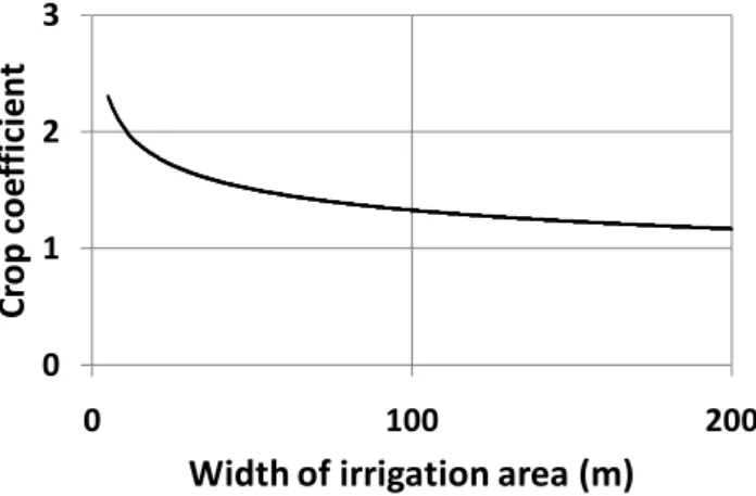
For small lakes and farm (and aesthetic) dams the in-creased evaporation at the upwind transition from a land en-vironment may need to be addressed. Using an analogy of evaporation from a small dish moving from a dry fallow landscape downwind across an irrigated cotton field, Mor-ton (1983, p. 78) noted that the decreased evaporation from the transition into the irrigated area (analogous to a lake) was associated with decreased air temperature and increased hu-midity. Morton (1983b, Eq. 11) recommends the following equation be used to adjust lake evaporation for the upwind advection effects:
ESLx=EL+(ETp−EL)
ln 1+x
C x C
, (23)
where ESLx is the average lake evaporation (mm day−1)
for a crosswind width ofx m,ELis lake evaporation (mm
day−1)large enough to be unaffected by the upwind
transi-tion, i.e. well downwind of the transitransi-tion, ETPis the potential
evaporation (mm day−1)of the land environment, andCis a
constant equal to 13 m.
Morton (1986, p. 379) recommends that ETPbe estimated
as the potential evaporation in the land environment as com-puted from CRWE and the lake evaporationELbe computed
from CRLE. ETP could also be estimated using Penman–