Adv. Sci. Res., 3, 113–118, 2009 www.adv-sci-res.net/3/113/2009/
©Author(s) 2009. This work is distributed under the Creative Commons Attribution 3.0 License.
Advances in
Science and
Research
EMS
Annual
Meeting
and
7th
Eur
opean
Confer
ence
on
Applied
Climatolo
gy
2008
Reference crop evapotranspiration estimate using
high-resolution meteorological network’s data
C. Lussana1and F. Uboldi2 1ARPA Lombardia, Milano, Italy 2Consultant, Novate Milanese, Italy
Received: 30 December 2008 – Revised: 8 May 2009 – Accepted: 20 May 2009 – Published: 12 October 2009
Abstract. Water management authorities need detailed information about each component of the hydrolog-ical balance. This document presents a method to estimate the evapotranspiration rate, initialized in order to obtain the reference crop evapotranspiration rate (ET0). By using an Optimal Interpolation (OI) scheme, the
hourly observations of several meteorological variables, measured by a high-resolution local meteorological network, are interpolated over a regular grid. The analysed meteorological fields, containing detailed meteoro-logical information, enter a model for turbulent heat fluxes estimation based on Monin-Obukhov surface layer similarity theory. The obtained ET0fields are then post-processed and disseminated to the users.
1 Introduction
Lombardia’s public environmental agency (ARPA Lombar-dia) has undertaken a number of projects aimed at improving knownledge of the water budget in order to support public authorities involved in water management. This document presents a procedure to estimate ET0, defined by Allen et al.
(1998) as the evapotranspiration rate for the hypothetical ref-erence crop (short grass with an ample supply of water).
ET0is a climatic parameter computed using
meteorolog-ical data only, without considering crop characteristics and soil factors.
The procedure’s outputs are ET0 hourly fields (unit
mm h−1). The estimated evapotranspiration rate can be
ag-gregated in time and space. Finally, the ET0 estimates are
published in a hydrological bulletin, which is disseminated to the users.
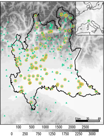
The source of meteorological information is ARPA Lom-bardia’s high-resolution meteorological network. The mete-orological variables used are hourly averaged values of tem-perature, relative humidity, wind components, solar global radiation and hourly cumulated precipitation values. The observing system is composed of about three hundred au-tomated weather stations. The stations spatial distribution presents strong inhomogeneities, moreover the sensor equip-ment vary from station to station. As an example, Fig. 1
Correspondence to: C. Lussana ([email protected])
shows the spatial distribution of thermometers and pyra-nometers.
The spatial domain of interest consists of the part of Po plain inside Lombardia’s administrative boundaries (see fields in Figs. 4 and 5). Elevations range from 10 m (in the south-eastern part) to less than 300 m (in the northern part). However, all the information available is used in the ET0
es-timation procedure in order to reduce border effects. Observations from the meteorological network are inter-polated over a regular grid with 1.5 km of resolution. For all variables except solar radiation, a statistical interpolation scheme is applied. At present, the interpolation of the hourly averaged solar global radiation is performed with a simple in-verse distance weighting method, Fig. 4 shows an example. An effort is made to prevent observations affected by gross errors from entering the interpolation procedure.
It is worthwhile remarking that the grid spatial resolution accounts for orographic details, but the interpolated fields can correctly reproduce phenomena resolved by the spatial resolution of the observational network, i.e. tenths of kilo-meters.
Once obtained the meteorological fields, a model for tur-bulent heat fluxes estimation is applied at each grid point. The model setup is such that the obtained latent heat flux co-incides with the energetic content associated to ET0.
Figure 1. Orography and station locations in the Lombardia do-main. Triangles: thermometers. Circles: pyranometers. The bold black line is the administrative boundary. The inset shows the geo-graphical location of Lombardia, longitude 8.5 to 11.5◦E, latitude
44.6 to 45.7◦N
2 Statistical interpolation
The statistical interpolation scheme is an implementation of the Optimal Interpolation (OI; Gandin, 1963). OI produces the best (in the sense of minimum analysis error variance), linear, unbiased estimate of the atmospheric field. The sta-tistical interpolation scheme is applied to hourly averaged values of temperature, relative humidity, wind and to hourly cumulated precipitation values. OI filters out the unresolved spatial scales. OI schemes often use a model-derived first guess, but the implementation reported here uses a back-ground field built by observations detrending, thus the pre-sented OI implementations are model-independent. Figure 2 shows temperature and relative humidity fields.
The description of the OI implementation for temperature and relative humidity can be found in Uboldi et al. (2008) while in Lussana et al. (2009) the application to other vari-ables is discussed and several test cases are reported. At present, with respect to that work, here the OI implemen-tation for precipiimplemen-tation uses raingauges measurements only, without the integration of radar-derived precipitation
esti-Figure 2. 28 July 2006, 18:00 UTC+1. Top: temperature (◦C).
Bottom: relative humidity (%).
mates. The background field is set to zero everywhere and the OI parameters maintain the analysis field as close as pos-sible to the observations: an example is shown in Fig. 3. The precipitation analysis plays an important role in the ET0
es-timation procedure, but only as a trigger: where the analyzed field of precipitation has a value greater than 1 mm h−1 the
ET0 value is not computed. In the future, the integration
Figure 3.28 July 2006, 18:00 UTC+1. Precipitation rate (mm h−1). The observed values are reported at station locations.
Figure 4. 28 July 2006, 18:00 UTC+1. Solar global radiation (W m−2).
3 Turbulent fluxes estimation
This Section presents a procedure to determine the surface moisture flux, using single-level meteorological data only. The moisture flux is intended as representative of an area rather than of a single roughness element. Due to the three-dimensional nature of turbulent vortices, the assumption of
Figure 5.28 July 2006. Daily cumulated ET0field (mm day−1 ) for the spatial domain of interest.
horizontal representativeness also imposes a constraint on the height above the ground where fluxes must be evaluated.
In fact, from the general Atmospheric Boundary Layer (ABL) theory, the Surface Layer (SL) (about 10% of the ABL vertical extension) can be divided in Roughness Sub-Layer (RSL) and Inertial Sub-Sub-Layer (ISL) (Garratt, 1994). The RSL – the lower portion of the SL – contains the canopy layer. On the one hand, turbulence in the RSL is influ-enced by individual roughness elements and the turbulence-related variables exhibit strong gradients in the vertical di-rection. On the other hand, turbulence in the ISL is influ-enced by the integrated effect of many roughness elements, thus the turbulence-related variables are representative of a larger area and the values of the turbulent fluxes are assumed to be constant with height. Most of Lombardia’s automatic stations are located within the ISL (in practice, only urban stations lie within the RSL). The meteorological fields enter-ing the procedure presented in the current session refer then to the ISL.
Based on the outlined structure of the SL, the evapotran-spiration rate is defined as the net rate of passage of water vapor across a horizontal reference plane inside the ISL.
Turbulence is the most efficient mechanism to exchange momentum, energy and mass inside the ABL. In the frame-work of turbulence theory it is more convenient to deal with the energetic content associated to the moisture flux: the tur-bulent latent heat flux He(W m−2). The evaporation rate E
(mm h−1) can be obtained by using: E∝ He
λρw
cially in case of tall canopies, also the zero-plane displace-ment height d must be introduced. Finally, the presence of ice and liquid water is not considered, then phase transitions are not taken into account.
The two turbulent heat fluxes, latent, He, and sensible, H0,
are related to the meteorological variables using the so-called scaling parameters:
H0 = −ρcpu∗T∗ (2)
He = −ρλu∗q∗ (3)
Whereρis the air density, cp is the specific heat at
con-stant pressure; u∗, T∗and q∗ are the scaling parameters for momentum, temperature and specific humidity, respectively. These last three parameters are (vertically) constant through all the ISL.
In analogy with Zdunkowski and Bott (2003), the Monin-Obukhov Similarity Theory (MOST) for the SL allows com-puting the scaling parameters through the iterative procedure:
u = u
(n)
∗ k
"
lnz−d z0 −
ΨM
z−d
L(n−1)
∗
!
+ ΨM
z0
L(n−1)
∗
!#
(4)
T −T0 =
T∗(n) k
"
lnz−d z0 −
ΨH
z−d
L(n−1)
∗
!
+ ΨH
z0
L(n−1)
∗
!#
(5)
q−q0 =
q(n)∗ k
"
lnz−d z0 −
ΨH
z−d
L(n−1)
∗
!
+ ΨH
z0
L(n−1)
∗
!#
(6)
L(n−1)
∗ = T gk u2 ∗ T∗
!(n−1)
, L(0)∗ =∞ (7)
Here u, T and q are the wind velocity, temperature and specific humidity, referred to the height above the ground z (in the ISL); k is the von Karman constant; L∗is the Monin-Obukhov length scale; n is the iteration index. The itera-tion stops when a prescribed accuracy for the L∗estimate is reached. The functionsΨare the characteristic functions for momentum (M) and heat (H) (Beljaars and Holtslag, 1991). The unknown temperature and specific humidity T0 and q0
are formally assigned to z0, but they must be intended as two
parameters characterizing the whole RSL.
In order to evaluate Eqs. (4)–(7), T0 and q0 are needed.
To obtain their values, a number of approximations must be
The resistances rHand rVhave the physical units of s m .
Both Eqs. (8) and (9) implicitly assume steady conditions. Equation (9) takes into account the evaporation originating from saturated surfaces in the RSL; the specific humidity dif-ference in Eq. (9) can be rewritten as a linearized function of temperature:
qs(T0)−q= ∆(T0−T )+δq (10)
Where∆≡∂qs/∂T is evaluated at a reference temperature
between T0and T . Moreover,δq≡qs(T )−q.
Referring to Monteith (1981), the resistance rHin Eq. (8)
is estimated by the aerodynamic resistance, rH≃ra, governing
the diffusion of energy and masses between RSL and ISL. rV
in Eq. (9) is estimated as rV≃ra+rs, where the surface
resis-tance rsis introduced to account for the evaporation and
tran-spiration processes in the RSL. In this work the “big-leaf” model is used: the canopy is treated as a plane located at the lower boundary of the RSL and the latent heat flux is deter-mined by the evaporation of liquid water from the “big-leaf”. With these assumptions, Eq. (9) is replaced by:
He=ρλ δq0
rs
(11) whereδq0≡qs(T0)−q0.
A further relation between the turbulent heat fluxes can be obtained from the overall surface energy balance. By means of the prognostic equation for entalphy applied to the earth surface, the energy balance can be written as (Zdunkowski and Bott, 2003):
Rn−G=H0+He (12)
Where Rn is the net radiation and G is the heat flux stored
in the soil. The left-hand side defines the available energy. Equation (12) is strictly valid for atmosphere-surface inter-face in case of bare soil. Nevertheless, Eq. (12) is intended as the energy balance equation at the canopy top because the horizontal flux of energy due to advection and the rate of en-ergy storage per unit area in the canopy layer are neglected. Therefore, the turbulent heat fluxes in Eq. (12) are assumed to be fluxes in the ISL and are interpreted as surface fluxes.
The net radiation is estimated using the Net All-wave Ra-diation Parameterization model (NARP; Offerle et al., 2003) while for G the expression G=βRnis used (β=0.1 for daytime
By making use of Eqs. (8)–(12), the turbulent heat fluxes are computed as (deRooy and Holtslag, 1999):
He =
∆
∆ +γ(Rn−G)+ ρcp
(∆ +γ) ra
(δq−δq0) (13)
H0 =
γ
∆ +γ(Rn−G)− ρcp
(∆ +γ) ra
(δq−δq0) (14)
Whereγ=cp/λis the psychrometric constant. Equations (13)
and (14) are used to overcome the problem of eliminating T0and q0inside the iterative procedure of Eqs. (4)–(7). The
iterative procedure is then rewritten as: u = u
(n)
∗ k
"
lnz−d z0 −
ΨM
z−d
L(n−1) ∗
!
+ ΨM
z0
L(n−1) ∗
!#
(15)
r(n)a = 1 ku(n)∗
"
lnz−d z0 −
ΨH
z−d
L(n−1) ∗
!
+ ΨH
z0
L(n−1) ∗
!#
(16)
δq(n)0 =
∆
∆+γ(Rn−G)+ ρcp
(∆+γ)ra(n)
δq
ρλ
rs +
ρcp
(∆+γ)ra(n)
(17)
H(n)0 = γ
∆ +γ(Rn−G)− ρcp
(∆ +γ) ra(n)
δq−δq(n)0
(18)
T∗(n) = − H
(n) 0
ρcpu(n)∗
(19)
L(n−1)
∗ = T gk u2 ∗ T∗
!(n−1)
, L(0)∗ =∞ (20)
For the iterative procedure, the three parameters z0, d and rs
need to be specified. Moreover, the albedo of the surface is required by the NARP model.
4 ET0estimation
The general method presented in Sect. 3 allows estimating the turbulent heat fluxes from single-level meteorological data. In order to obtain ET0, the parameters in the
proce-dure must be properly initialized. In Allen et al. (1998) the reference crop is defined as grass with height h=0.12m and albedo equals to 0.23. Furthermore, the relation for the sur-face roughness parameters are indicated as z0=0.123 h and
d=2/3 h. With respect to the rsvalue, in a review of the FAO
method for hourly period Allen et al. (2006) suggest using rs=50 s m−1 during daytime and rs=200 s m−1 during
night-time. The ET0 value is not computed for grid points where
the hourly precipitation rate is greater than 1mm h−1because
in case of rain the assumptions made in Sect. 3 are not justi-fied. Figure 5 shows a field of daily cumulated ET0, obtained
by summing up the hourly ET0estimates.
5 Conclusions
The presented procedure for ET0 estimation relies on the
availability of interpolated meteorological fields and com-bines these fields with a model for turbulent fluxes estimation near the ground, properly initialized.
The amount of information that contribute to the produc-tion of a ET0hourly field is remarkable, in consideration of
the domain extension. In fact, about one thousand of mete-orological observations are used every hour. The quality of the input meteorological fields is of crucial importance. The OI implementations for the meteorological variables provide reliable and detailed meteorological fields. However, the es-timate of solar global radiation over the domain must be im-proved.
The outputs of the turbulent fluxes estimation model must be compared with experimental data. Nevertheless, prelimi-nary qualitative evaluations are very encouraging.
In principle, the turbulent fluxes estimation procedure could be set up to obtain the real evapotranspiration rate for the actual crop. This would imply a more complex treatment of both the available geographical information and the veg-etation behaviour, as a consequence several complementary parameters would need to be tuned. It would be thus possi-ble to compare hourly estimates with the evapotranspiration estimates obtained using, for example, the approach of Allen et al. (2006), then possibly obtain some insights about crop coefficient values.
Edited by: E. Koch
Reviewed by: two anonymous referees
References
Allen, R. G., Pereira, L. S., Raes, D., and Smith, M.: Crop evap-otranspiration – Guidelines for computing crop water require-ments – FAO Irrigation and drainage paper 56, FAO – Food and Agriculture Organization of the United Nations, 1998.
Allen, R. G., Pruitt, W. O., Wright, J. L., Howell, T. A., Ventura, F., Snyder, R., Itenfisu, D., Steduto, P., Berengena, J., Yrisarry, J. B., Smith, M., Pereira, L. S., Raes, D., Perrier, A., Alves, I., Walter, I., and Elliott, R.: A recommendation on standardized surface resistance for hourly calculation of reference ETo by the FAO56 Penman-Monteith method, Agricultural Water Management, 81, 1–22, 2006.
Beljaars, A. and Holtslag, A.: Flux parameterization over land sur-faces for atmospheric models, J. Appl. Meteorol., 30, 327–341, 1991.
deRooy, W. C. and Holtslag, A.: Estimation of Surface Radiation and Energy Flux Densities from Single-Level Weather Data, J. Appl. Meteorol., 38, 526–540, 1999.
Gandin, L. S.: Objective Analysis of Meteorological Fields, Gidromet, Leningrad. English translation by Israeli Program for Scientific Translations, Jerusalem, 1963.
Garratt, J.: The atmospheric boundary layer, Cambridge University Press, 1994.
Lussana, C., Salvati, M. R., Pellegrini, U., and Uboldi, F.: Efficient high-resolution 3-D interpolation of meteorological variables for operational use, Adv. Sci. Res., 3, 105–112, 2009.