R. N. Elias
A. L. G. A. Coutinho and
M. A. D. Martins
Center for Parallel Computations and Department of Civil Engineering Federal University of Rio de Janeiro P. O. Box 68506 21945-970 Rio de Janeiro, Rj Rio de Janeiro, RJ. Brazil {renato, alvaro, marcos}@nacad.ufj.br
Inexact Newton-Type Methods for
Non-Linear Problems Arising from the
SUPG/PSPG Solution of Steady
Incompressible Navier-Stokes
Equations
The finite element discretization of the incompressible steady-state Navier-Stokes equations yields a non-linear problem, due to the convective terms in the momentum equations. Several methods may be used to solve this non-linear problem. In this work we study Inexact Newton-type methods, associated with the SUPG/PSPG stabilized finite element formulation. The resulting systems of equations are solved iteratively by a preconditioned Krylov-space method such as GMRES. Numerical experiments are shown to validate our approach. Performance of the nonlinear strategies is accessed by numerical tests. We concluded that Inexact Newton-type methods are more efficient than conventional Newton-type methods.
Keywords: Inexact Newton-type methods, Newton-Krylov methods, Navier-Stokes, incompressible fluid flow, finite elements
Introduction
We consider the simulation of incompressible fluid flow governed by Navier-Stokes equations using the stabilized finite element formulation proposed by Tezduyar (1991). This formulation allows that equal-order-interpolation velocity-pressure elements are employed, circumventing the Babuska-Brezzi stability condition by introducing two stabilization terms. The first term is the Streamline Upwind Petrov-Galerkin (SUPG) presented by Brooks & Hughes (1982) and the other one is the Pressure Stabilizing Petrov Galerkin (PSPG) stabilization proposed initially by Hughes et al (1986) for Stokes flows and later generalized by Tezduyar (1991) to finite Reynolds number flows. SUPG/PSPG implementations have been very successful in the simulation of complex, large scale fluid flow problems in parallel computers (Tezduyar et al, 1993, 1996). Nowadays it has been used for simulations of 3D fluid-structure interaction problems on unstructured grids with more than one billion of elements (Aliabadi et al, 2002). Usually the resulting fully coupled (velocity-pressure) linearized systems of equations are solved by a preconditioned Krylov-space iterative method such as GMRES (Saad, 2003).1
If we restrict ourselves to the steady case, it is known that, when discretized, the incompressible Navier-Stokes equations give rise to a system of nonlinear algebraic equations due the presence of convective terms in the momentum equations. Among several strategies to solve nonlinear problems the Newton’s methods are attractive because it converges rapidly from any sufficient good initial guess (Dembo et al, 1982), (Kelley, 1995). However, the implementation of Newton’s method involves some considerations: determining steps of Newton’s method requires the solution of linear systems at each stage and exact solutions can be too expensive if the number of unknowns is large. In addition, the computational effort spent to find exact solutions for the linearized systems may not be justified when the nonlinear iterates are far from the solution. Therefore, it seems reasonable to use an iterative method (Barret et al, 1994), such as BiCGSTAB or GMRES, to solve these linear systems only approximately.
Paper accepted September, 2004. Technical Editor: Aristeu Silveira Neto.
The inexact Newton method associated with a proper iterative Krylov solver, presents an appropriated framework to solve nonlinear systems, offering a trade-off between accuracy and amount of computational effort spent per iteration. For a proper mathematical description of the inexact Newton method we refer to Kelley (1995). It is often necessary to increase the robustness of the inexact Newton method adding some globalization procedure (Kelley, 1995, Pernice et al, 1998).
In the context of the SUPG/PSPG formulation for the steady incompressible Navier-Stokes equations coupled with heat and mass transfer, the work of Shadid et al (1997) investigated in depth the behavior of the inexact Newton method with backtracking. They have shown its computational efficiency and robustness. However, they pointed out that globalization by backtracking may be less robust when high accuracy is required at each linear solve than when less accuracy is required. A mathematical explanation for this behavior is provided in Tuminaro et al (2002). In the works of Shadid et al (1997) and Tuminaro et al (2002) the Jacobian was evaluated by a mixed method. Contributions emanating from the Galerkin term were computed analytically, whereas contributions from the stabilization terms were evaluated by numerical differentiation.
In this work, we evaluate the effectiveness of some Newton-type methods dealing with problems involving steady incompressible fluid flows. We also investigate the influence of the Jacobian form described by Tezduyar (1999). This form is based on Taylor's expansions of the nonlinear terms and presents an alternative and simple way to implement the tangent matrix employed by inexact Newton-type methods. The Krylov-subspace iterative driver of the Newton-type algorithms is a nodal-block diagonal preconditioned element-by-element GMRES solver. The test problems are the well-known driven cavity flow and flow over a backward facing step.
Governing Equations and Finite Element Formulation
Let Ω ⊂ ℜnsd be the spatial domain, where n
sd is the number of space dimensions. Let Γ = ΓgUΓh denote the boundary of Ω. We consider the following velocity-pressure formulation of the Navier-Stokes equations governing steady incompressible flows,
(
)
onρ ⋅u ∇∇∇∇u− − ⋅f ∇ σ = 0∇ σ = 0∇ σ = 0∇ σ = 0 Ω (1)
on
⋅ Ω
∇ = 0 ∇∇ = 0= 0
∇ u= 0 (2)
where ρ and u are the density and velocity respectively, and σσσσ is the stress tensor given as
σσσσ
( )
p,u = − Ι + 2 ε= − Ι + 2 ε= − Ι + 2 ε= − Ι + 2 εp µ( )
u , (3)with,
( )
+( )
T
1111 2222
ε = ∇ ∇
ε = ∇ ∇
ε = ∇ ∇
ε u = ∇u ∇u . (4)
Here, p and µ are the pressure and dynamic viscosity, and I is the identity tensor. The essential and natural boundary conditions associated with equations (1) and (2) are represented as
onΓ
==== g
u g (5)
on
⋅σ =σ =σ =σ = Γh
n h . (6)
Let us assume following Tezduyar (1991) that we have some suitably defined finite-dimensional trial solution and test function spaces for velocity and pressure, Suh, Vuh, Shp and =
h h
p p
V S . The stabilized finite element formulation of equations (1) and (2) can then be written as follows: Find uh∈Suh and ∈
h h
p
p S such that
∀ h∈Vh u
w and ∀ ∈qh Vph:
(
)
( ) (
)
h h h h h h h h
:
d p , d q d
ρ
Ω Ω Ω
⋅ ⋅ − Ω + Ω + ⋅ Ω
∫
w u ∇∇∇∇u f∫
εεεε w σσσσ u∫
∇∇∇∇ u(
)
(
)
1
τ ρ ρ
= Ω
+
∑∫
el ⋅∇∇∇∇ ⋅ ⋅∇∇∇∇ − ⋅∇ σ∇ σ∇ σ∇ σ − Ωn
h h h h h h
SUPG e
p , d
u w u u u f
(
)
(
)
1
1
τ ρ ρ
ρ = Ω
+
∑∫
nel ∇∇∇∇ h⋅ h⋅∇∇∇∇ h − ⋅∇ σ∇ σ∇ σ∇ σ h h − ΩPSPG e
q u u p ,u f d
h
Γ
=
∫
w ⋅hdΓ (7)In the above equation the first three integrals on the left hand side and the right hand side integral represent terms that appear in the standard Galerkin formulation of the problem (1)-(6), while the remaining integral expressions represent the additional terms which arise from the stabilized finite element formulation of the problem. Note that the stabilization terms are evaluated as the sums of element-wise integral expressions. The first summation corresponds to the SUPG (Streamline Upwind Petrov/Galerkin) term and the second correspond to the PSPG (Pressure Stabilization Petrov/Galerkin) term. We have calculated the stabilization parameters (Tezduyar et al, 1992) as follows,
( )
1 2 2 2
2
2 4
9 ν
τ τ
−
= = +
h
SUPG PSPG #
#
h h
u
(8)
Here u h is the local velocity vector, ν represent the kinematic viscosity and h# is the element length, defined to be equal to the diameter of the circle which is area-equivalent to the element. The spatial discretization of equation (7) leads to the following set of non-linear algebraic equations,
( )
( )
(
)
( )
δ δ
ϕ ϕ
+ + − + =
+ + = p
p
p
T
u
N u N u Ku G G f
G u N u G f (9)
where u is the vector of unknown nodal values of uh and p is the
vector of unknown nodal values of ph. The non-linear vectors
( )
N u , Nδ
( )
u , and Nϕ( )
u the matrices K, G, Gδδδδ and Gϕ emanate, respectively, from the convective, viscous and pressure terms. The vectors fu and fp are due to the boundary conditions(5) and (6). The subscripts δ and ϕ identify the SUPG and PSPG contributions respectively. In order to simplify the notation we denote by x=
( )
u,p a vector of nodal variables comprising both nodal velocities and pressures, thus, equation (9) can be written as,( )
=F x 0 (10)
where F x
( )
represents a nonlinear vector function.For Reynolds numbers much greater than unity the nonlinear character of the equations becomes dominant, making the choice of the solution algorithm, especially with respect to its convergence and efficiency, a key issue. The search for a suitable nonlinear solution method is complicated by the existence of several procedures and their variants. In the following section we present the nonlinear solution strategies based on the Newton-type methods which are evaluated in this work.
Nonlinear Solution Procedures
Consider the nonlinear problem arising from the discretization of the fluid flow equations described by equation (10). We assume that F is continuously differentiable in ℜnsd and denote its
Jacobian matrix by F'∈ℜnsd. The Newton’s method is a classical
algorithm for solving equation (10) and can be enunciated as: Given an initial guess x0, we compute a sequence of steps sk and iterates
k
x as follows,
Algorithm N
FOR k=0 STEP 1 UNTIL “Convergence” DO:
Solve F x'
( )
k sk= −F x( )
k (11)Set xk+1=xk+sk
unknowns is large and may not be justified when xk is far from a solution. Thus, one might prefer to compute some approximate solution, leading to the following algorithm:
Algorithm In
FOR k=0 STEP 1 UNTIL “Convergence” DO: FIND someη ∈k 0 1,
)
AND sk THAT SATISFY( )
k + '( )
k k ≤ηk( )
kF x F x s F x (12)
Set xk+1=xk+sk
for some η ∈k 0 1,
)
, where • is a norm of choice. This formulation naturally allows the use of an iterative solver: one first chooses ηk and then applies the iterative solver to equation (11) until a sk is determined for which the residual norm satisfies equation (12) In this context ηk is often called the forcing term, since its role is to force the residual of (11) to be suitably small. This term can be specified in several ways (see, Eisenstat & Walker, 1996, Shadid et al, 1997, Pernice et al, 1998) to enhance efficiency and convergence and will be treated in the following section below. In our implementation we have used the nodal block-diagonal preconditioned GMRES(m) method to solve the Newton equations (11), where m represents the number of basis vectors used by GMRES algorithm (Saad, 2003).A particularly simple scheme for solving the nonlinear system of equations (10) is a fixed point iteration procedure also known as the successive substitution, the Picard iteration, functional iteration or successive iteration. Note in the algorithms above that if we do not build the Jacobian matrix in equations (11) and (12) and the solution of previous iterations were reused, we have a successive substitution (SS) method. In this work, we have evaluated the efficiency of Newton and successive substitution methods and their inexact versions. We may also define a mixed strategy combining SS and N (or ISS and IN) iterations, to improve performance, as discussed in the following. In this strategy the Jacobian evaluation is enabled after k successive substitutions. Thus, we have labeled the mixed strategy as k-SS+N or as k-ISS+IN in the case of its inexact counterpart.
Forcing Term
We have implemented the forcing term as a variation of the choice from Eisenstat & Walker (1996) that tends to minimize oversolving while giving fast asymptotic convergence to a solution of (10). Oversolving means that the linear equation for the Newton step is solved to a precision far beyond what is needed to correct the nonlinear iteration. Kelley (1995) considered the following measure of the degree to which the nonlinear iteration approximates the solution,
( )
2( )
21
ηka=γ F xk F xk− , (13)
where γ ∈0 1,
)
is a parameter. In order to specify the choice at 0=
k and bound the sequence away from 1 we set
(
)
00η η
η η
=
=
>
max b
k a
max k
k ,
min , k . (14)
Here the parameter ηmax is an upper limit of the sequence {ηka}. We have chosen γ= 0.9 according to Eisenstat & Walker (1996) and adopted ηmax = 0.9, 0.5, 0.1 arbitrarily in our tests.
It may happen that ηb
k is small for one or more iterations while xk is still far from the solution. A method of safeguarding against
this possibility was suggested by Eisenstat & Walker (1996) to avoid volatile decreases in ηk. The idea is that if ηk-1 is sufficiently large we do not let ηk decrease by much more than a factor of ηk-1, that is:
(
)
(
)
(
)
2 1
2 2
1 1
0
0 0 1
0 0 1
η
η η η γη
η η γη γη
−
− −
=
= > <
> >
max
c a
k max k k
a
max k k k
k ,
min , k , . ,
min ,max , k , . ,
(15)
The constant 0.1 is arbitrary. According to Kelley (1995) the safeguarding does improve the performance of the iteration.
There is a chance that the final iterate will reduce F far beyond the desired level, consequently the cost of the solution of the linear equation for the last step will be higher than really needed. This oversolving in the final step can be controlled comparing the norm of the current nonlinear residual to the nonlinear norm at which the iteration would terminate
0
τNL=τres F (16)
and bounding ηk by a constant multiple of τNL F x
( )
k . We haveused the choice proposed by Kelley (1995)
( )
(
)
(
0 5)
η = η ηc τ
k min max,max k, . NL F xk (17)
where τNL represent the nonlinear tolerance.
Backtracking Procedures
The backtracking procedures are employed, in the context of nonlinear methods, to improve the convergence capability for any initial guess (Eisenstat & Walker, 1994). These procedures, also known as line searches or globalization procedures are based on trying to recover the convergence of a nonlinear method performing reductions on a Newton step according to the evolution of nonlinear residual. There are several forms to impose these step reductions and a constant reduction is often employed successfully, but sometimes disturbing the nonlinear convergence. In this work we employ the Armijo rule as described in Kelley (1995). This rule tries to compute a sufficient Newton step reduction without disturbing the nonlinear convergence, according to a residual decreasing function (see Kelley, 1995). Thus we may describe the Armijo rule by the procedures below.
After rejecting j step reductions we have the following sequence:
( )
2(
1)
2(
1)
2
λ λ−
+ +
k , k k ,... k j k
F x F x s F s s (18)
( )
λ =(
k+λ k)
2f F x s . (19)
The minimal of the function (19) can be used for computing the next step reduction. According to Kelley (1995), we have used a third order polynomial to compute the step reduction. This procedure can be summarized as: After reject λc and build the polynomial model we compute the minimal of λt analytically and the following adjustment is performed,
0 0
1 1 1
if if otherwise
σ λ λ σ λ
λ σ λ λ σ λ
λ +
<
= >
c t c
j c t c
t
,
, (20)
In a 3-point parabolic model, the procedure for evaluating f (0) and f (1) is performed by the following steps. If the step for λ =1 was rejected, adjust λ = σ1 and try again. After the second step
rejection, we have the following values to construct the 3-point parabolic model,
( )
0( )
λc and( )
λjf , f f , (21)
where λc and λj are the values of λ most recently rejected. The interpolation polynomial of f at the points 0, λc, λj is,
( ) ( )
(
)
(
( ) ( )
0)
(
)
(
( )
( )
0)
pλ 0 λ λ λ λ λ λ λ
λ λ λ λ
− − − − = + + − c j j c
j c j
f f
f f
f .
(22)
We must evaluate two possibilities for the curvature of polynomial in equation (22). Thus we have,
( )
2(
(
( ) ( )
)
(
( )
( )
)
)
p 0 λ λ λ λ 0 λ λ 0
λ λ
= − − −
−
c j
j c c j
c j
" f f f f , (23)
and
( )
( )
p 0
p 0
λ = −t '
" . (24)
If the curvature of p is positive, set λt to the minimal of p and compute λj+1 by equation (20); otherwise p"
( )
0 ≤0, set λj+1 as the minimal of p in the interval [σ0λ, σ1λ] or reject the parabolic modeland set λj+1 as σ0λ or σ1λ. In this work we adopted the second
strategy, setting λj+1 = σ1λ.
Jacobian Matrix Evaluation
To form the Jacobian F' required by Newton-type methods we use a numerical approximation described by Tezduyar (1999). Consider the following Taylor expansion for the nonlinear convective term emanating from the Galerkin formulation:
(
+)
=( )
+∂ +∂
∆ ∆
∆ ∆
∆ ∆
∆ N∆ ...
N u u N u u
u (25)
where ∆∆∆∆u is the velocity increment. Discarding the high order terms and omitting the integral symbols we arrive to the following approximation,
(
) (
)
(
)
(
)
(
)
ρ ρ ρ ρ + ⋅ + ≅ ⋅ + ⋅ + ⋅ ∆ ∇ ∆ ∇ ∆ ∇ ∆ ∇ ∆ ∇ ∆ ∇ ∆ ∇ ∆ ∇ ∇ ∆ ∆ ∇ ∇ ∆ ∆ ∇ ∇ ∆ ∆ ∇ ∇ ∆ ∆ ∇u u u u u u
u u u u
(26)
Note that the first term in the right hand side of equation (26) is the corresponding residual vector and the remaining terms represent the numerical approximation of ∂N∂u. If we apply similar derivations to Nδ (u) and Nϕϕϕϕ (u) we obtain,
(
)
(
) (
)
(
) (
)
(
) (
)
(
) (
)
(
) (
)
τ ρ
τ ρ τ ρ
τ ρ τ ρ
+ ⋅∇ ⋅ + ⋅∇ + ≅ ⋅ ∇ ⋅ ⋅ ∇ + ⋅∇ ⋅ ⋅∇ + ⋅ ∇ ⋅ ⋅ ∇ + ⋅ ∇ ⋅ ⋅∇ ∆ ∆ ∆ ∆∆ ∆∆ ∆∆ ∆ ∆ ∆ ∆∆∆∆ ∆ ∆ ∆∆ ∆∆ ∆ ∆ SUPG SUPG SUPG SUPG SUPG
u u w u u u u
u w u u u w u u
u w u u u w u u
(27)
and
(
) (
)
(
)
(
)
(
)
τ
τ τ τ
⋅ + ⋅ + ≅ ⋅ ⋅ + ⋅ ⋅ + ⋅ ⋅ ∇ ∆ ∇ ∆ ∇ ∆ ∇ ∆ ∇ ∆ ∇ ∆ ∇ ∆ ∇ ∆ ∇ ∇ ∇ ∆ ∇ ∇ ∇ ∆ ∇ ∇ ∇ ∆ ∇ ∇ ∇ ∆ ∇ ∇ ∇ ∆ ∇ ∇ ∇ ∆ ∇ ∇ ∇ ∆ ∇ ∇ ∇ ∆ PSPG
PSPG PSPG PSPG
u u u u
u u u u u u
q
q q q
(28)
where again the first terms in the right hand side of equations (27) and (28) are the SUPG and PSPG contributions to the residual vector and the remaining terms define the approximations of ∂ δ
∂ N
u
and ∂Nϕ∂u.
We do not assemble and store the resulting Jacobian, but rather we compute its action in the matrix-vector product needed in GMRES from element contributions, that is,
1 = ′ = nel ' e e e
F x
A
F x (29)where
A
is the standard finite element assembly operator (Hughes, 2000), Fe′ is the e-th contribution for the global Jacobian and xe isthe restriction of a general search direction to the element degrees of freedom. A similar strategy is employed in the successive substitution methods.
Test Problems
In this section we present the results obtained with the formulation described in the previous sections applied to two classical CFD problems. The first example consists of the lid driven cavity flow and the second is the flow over a backward facing step. For both examples we have tested the nonlinear algorithms proposed at Reynolds numbers 100, 500 and 1000. The numerical procedure considers a fully coupled u-p version of stabilized formulation using linear triangular elements. The computations were halted when the
following criteria were met: 3
0 10
− ≤
F F and 3
10−
≤
s x or
the total number of nonlinear iterations exceeds 1000.
Lid Driven Cavity flow
of the cavity, the flow velocity on the lid and fluid viscosity. The problem domain and mesh with 1,681 nodes and 3,200 elements are presented in Figs. 1a and 1b respectively.
ux = 1, uy = 0
=
x
u uy = 0
0.0 1.0
= 0
y
u 0 =
x
u ux = 0
= 0
y
u
0.0 1.0
(a)
(b)
Figure 1. Two-dimensional lid-driven cavity problem – (a) Domain Problem, (b) Finite element mesh (1,681 nodes and 3,200 elements).
Table 1 shows the results for tests with different nonlinear strategies to solve the lid driven cavity flow at Reynolds number 100, 500 and 1000. In all tests we employed GMRES(45) with nodal block-diagonal preconditioning to solve the linear problem. For the classical Newton-type methods the linear solver tolerance was set to 10-6. For the inexact methods we have tested 0.1, 0.5 and 0.9 as the maximum linear solver tolerance, ηmax. For each Table presented in this section, the first column lists the nonlinear method employed, where SS and ISS-η labels represent the Successive Substitution and Inexact Successive Substitution methods respectively and η is the maximum linear solver tolerance adopted by the inexact method. The second column shows the number of linear iterations (# LI) performed by GMRES. The third column gives the number of nonlinear iterations (# NLI) performed by each method. The fourth column presents the time spent in the solution process and the Euclidean solution norms (
2
• ) were presented on the three last columns as solution quality indicators. Some Tables present two additional columns with the label (INFO) comprising warning messages or information about the solution process and (BCT) with the number of backtracking steps performed.
Table 1. Performance of Successive Substitution and Inexact Successive Substitution. Influence of the maximum linear solver tolerance. GMRES(45), Re = 100, 500 and 1000.
# LI # NLI Time
(s) || ux ||2 || uy ||2 || p ||2
Re = 100
SS 8668 5 38.0 10.6873 5.6228 5.4948 ISS-0.1 1388 7 6.08 10.6873 5.6210 5.4783 ISS-0.5 1174 13 5.15 10.6862 5.6183 5.4748 ISS-0.9 779 11 3.40 10.6826 5.5825 5.4686
Re = 500
SS 11678 7 50.8 9.6971 5.7740 2.2638 ISS-0.1 1831 14 8.05 9.6979 5.7738 2.2163 ISS-0.5 1142 23 5.03 9.6974 5.7687 2.2114 ISS-0.9 968 41 4.28 9.6972 5.7600 2.2065
Re = 1000
SS 19850 11 86.3 9.0300 5.2626 1.5739 ISS-0.1 1685 14 7.37 9.0318 5.2653 1.5234 ISS-0.5 1199 28 5.27 9.0345 5.2681 1.5162 ISS-0.9 905 39 4.01 9.0342 5.2689 1.5182
We can see in Table 1 that although the classical SS method requires less nonlinear iterations, it needed more GMRES iterations and thus, it is slower than the inexact method. We also observe that increasing the Reynolds number the solution process becomes more difficult.
Table 2 presents a performance comparison among the Newton-type implementations described in previous sections. These Newton-type methods differ by the form on which the Jacobian matrix evaluation is performed in the linearized problem. In the ISS method the nonlinear derivatives are not evaluated during the solution process. In the inexact Newton method (IN) the approximated Jacobian matrix is built and evaluated using the expressions in equations (26) to (28) from the start to the end of the nonlinear solution. We may also use a mixed solution strategy to circumvent initialization problems observed in some problems. In this strategy we enable the approximate Jacobian evaluation after k successive substitutions, thus this method will be labeled as k -ISS+IN. We have adopted arbitrarily in our tests k=5 and
0 1
ηmax= . .
Table 2. Performance of the Newton-type methods. GMRES(45), ηηηηmax = 0.1,
Re = 100, 500 and 1000.
# LI # NLI Time
(s) || ux ||2 || uy ||2 || p ||2
Re = 100
ISS 1388 7 6.05 10.6873 5.6210 5.4783 IN 1400 5 6.12 10.6871 5.6224 5.4794 5-ISS+IN 1543 7 6.67 10.6871 5.6224 5.4787
Re = 500
ISS 1832 14 8.00 9.6979 5.7738 2.2163 IN 1952 10 8.54 9.6970 5.7739 2.7762 5-ISS+IN 1405 9 6.05 9.6970 5.7739 2.2162
Re = 1000
ISS 1685 14 7.30 9.0318 5.2653 1.5234 IN 42818 12 186.0 9.0306 5.2636 1.5995 5-ISS+IN 1488 10 6.39 9.0308 5.2639 1.5230
be associated to an ill-conditioning of the resulting numerically approximated Jacobian. Figs 2a to 2c show the residual decay per iteration for each strategy in Table 2.
0 1 2 3 4 5 6 7 8
-5.5 -5.0 -4.5 -4.0 -3.5 -3.0 -2.5 -2.0 -1.5 -1.0 -0.5
lo
g1
0
(
|
|
r
|
|
/
|
|
r0
|
|
)
NONLINEAR ITERATIONS
ISS IN 5-ISS+ IN
(a) Reynolds 100
0 1 2 3 4 5 6 7 8 9 10 11 12 13 14 15 -5.5
-5.0 -4.5 -4.0 -3.5 -3.0 -2.5 -2.0 -1.5 -1.0 -0.5 0.0 0.5 1.0 1.5
lo
g1
0
(
|
|r
|
|
/
|
|r
0
||
)
NONLINEAR ITERATIONS
ISS IN 5-ISS+ IN
(b) Reynolds 500
0 1 2 3 4 5 6 7 8 9 10 11 12 13 14 15 -6.0
-5.5 -5.0 -4.5 -4.0 -3.5 -3.0 -2.5 -2.0 -1.5 -1.0 -0.5 0.0 0.5 1.0
lo
g1
0
(
|
|r
||
/
|
|r0
||
)
NONLINEAR ITERATIONS
ISS IN 5-ISS+ IN
(c) Reynolds 1000
Figure 2. Convergence history - Influence of numerical Jacobian evaluation in Newton-type methods.
We can note in these Figures that for increasing Reynolds numbers convergence deteriorates. These Figures also show that convergence is faster for the methods based in the numerically approximated Jacobian evaluations than for the successive substitution methods.
In Table 3 we present the results of inexact nonlinear methods with backtracking enabled. Note that backtracking was invoked only for Re=500 and 1000. It was particularly important for recovering accuracy and reducing processing times of the IN solutions.
Table 3. Performance of inexact methods with globalization (backtracking)
procedures. GMRES(45), ηηηηmax = 0.1, Re = 100, 500 and 1000.
# LI # NLI
Time
(sec) #BCT || ux ||2 || uy ||2 || p ||2
Re = 100
ISS 1388 7 6.0 0 10.687 5.621 5.478
IN 1401 5 6.1 0 10.687 5.622 5.479
5-ISS+IN 1543 7 6.7 0 10.687 5.622 5.479
Re = 500
ISS 1831 14 7.9 0 9.698 5.774 2.216
IN 1478 7 6.4 2 9.697 5.774 2.216
5-ISS+IN 1405 9 6.1 0 9.697 5.774 2.216
Re =
1000
ISS 1783 14 7.8 1 9.032 5.266 1.514
IN 1641 9 7.1 3 9.031 5.263 1.524
5-ISS+IN 1339 9 5.8 1 9.031 5.265 1.513
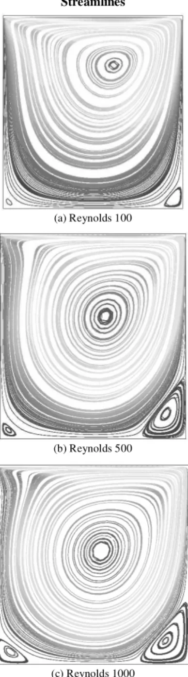
Figures 3 and 4 show the results obtained with the nonlinear methods for Reynolds numbers 100, 500 and 1000. These results were obtained with the inexact successive substitution method. Note in these Figures the vortex displacement for the center of the square for increasing Reynolds numbers.
Velocity
(a) Reynolds 100
(b) Reynolds 500
(c) Reynolds 1000
Streamlines
(a) Reynolds 100
(b) Reynolds 500
(c) Reynolds 1000
Figure 4. Steady-state solution for the lid-driven cavity flow.
Flow Over a Backward Facing Step
As a second example we consider the flow over a backward facing step, which also has become popular as a test problem for flow simulation codes. It consists of a fluid flowing into a straight channel which abruptly widens on one side. Numerical results obtained using a wide range of methods can be found in Gartling (1990). When the fluid flows downstream, it produces a
recirculation zone on the lower channel wall, and for sufficiently high Reynolds it also produces a recirculation zone farther downstream on the upper wall. The finite element mesh with 1,800 elements and 1,021 nodes, boundary conditions and problem domain are present in Fig. 5a-b. Note that the Fig. 5a shows only the part of the computational domain that contains all the essential features.
= 0
y
u
1 =
x
u
=
ux uy = 0
x
u= = 0 uy
0.0 7.5 30.0
0.75
0.0 1.5
(a)
(b)
Figure 5. Flow over a backward facing step. (a) Problem domain and (b) finite element mesh (1,800 elements and 1,021 nodes).
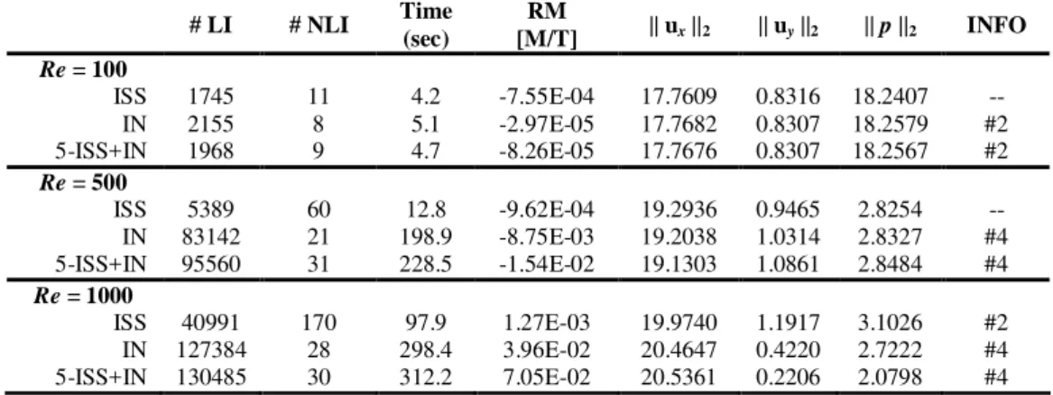
Table 4 presents the performance results obtained for the Newton-type methods. The definitions adopted here are the same employed in the previous example. The additional column identified by RM, means one more quality parameter. It represents the Residual Mass found for the incompressibility constraint given by equation (2).
Here again, we observe that the inexact methods needed more nonlinear iterations. As in the previous example, these iterations required less time. Observe that for Reynolds 1000, only SS and ISS-0.1 methods were able to solve this problem for all variables. We note that the classical methods were more conservative, presenting less residual mass than the inexact methods. However, the residual mass of the converged inexact Newton solutions are of the same order of the required nonlinear accuracy. Table 5 shows the results obtained for the numerical Jacobian influence tests applied to the backward facing step problems. The tolerances and the other parameters were the same employed in the lid driven cavity flow problem.
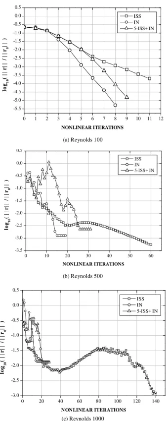
Table 5 shows that the methods based on numerical Jacobian evaluations needed less nonlinear iterations. However, these methods were less efficient, spending more time than successive substitution methods. Also in this case the methods based on numerical Jacobian evaluations were less accurate for high Reynolds numbers, as indicated in Table 5. Figure 6 presents the residual decays for the backward facing step problems.
Table 4. Performance of Successive Substitution and Inexact Successive Substitution. Influence of the maximum tolerance choice. GMRES(45), Re = 100, 500 and 1000.
# LI # NLI Time (s) RM
[M/T] || ux ||2 || uy ||2 || p ||2 INFO
Re = 100
SS 11689 7 27.9 2.70E-08 17.7681 0.8313 18.2585 --
ISS-0.1 1745 11 4.2 -7.55E-04 17.7609 0.8316 18.2407 --
ISS-0.5 1446 22 3.5 -1.92E-03 17.7504 0.8310 18.2157 --
ISS-0.9 1218 36 3.0 -4.92E-03 17.7185 0.8312 18.1392 --
Re = 500
SS 33278 19 79.4 4.57E-08 19.2898 0.9705 2.8084 --
ISS-0.1 5389 60 13.0 -9.62E-04 19.2936 0.9465 2.8254 --
ISS-0.5 3918 162 9.3 -4.07E-03 19.2633 0.9742 2.8397 --
ISS-0.9 4051 495 10.5 -4.97E-03 19.2546 0.9892 2.8418 #2
Re = 1000
SS 1931600 65 4597.3 -9.63E-08 19.9767 1.1787 3.1130 #2
ISS-0.1 40991 170 98.0 1.27E-03 19.9740 1.1917 3.1026 #2
ISS-0.5 96615 1000 233.0 -3.72E-02 20.1701 0.7343 3.4210 #1
ISS-0.9 13306 1000 35.2 1.02E-01 20.6229 0.1962 1.6459 #1
#1 - Nonlinear method reached the maximum number of iterations without converging. #2 – GMRES(45) reached the maximum number of iterations without converging in some nonlinear step.
Table 5. Performance of the Newton-type methods. GMRES(45), ηηηηmax = 0.1, Re = 100, 500 and 1000.
# LI # NLI Time
(sec)
RM
[M/T] || ux||2 || uy ||2 || p ||2 INFO Re = 100
ISS 1745 11 4.2 -7.55E-04 17.7609 0.8316 18.2407 --
IN 2155 8 5.1 -2.97E-05 17.7682 0.8307 18.2579 #2
5-ISS+IN 1968 9 4.7 -8.26E-05 17.7676 0.8307 18.2567 #2
Re = 500
ISS 5389 60 12.8 -9.62E-04 19.2936 0.9465 2.8254 --
IN 83142 21 198.9 -8.75E-03 19.2038 1.0314 2.8327 #4
5-ISS+IN 95560 31 228.5 -1.54E-02 19.1303 1.0861 2.8484 #4
Re = 1000
ISS 40991 170 97.9 1.27E-03 19.9740 1.1917 3.1026 #2
IN 127384 28 298.4 3.96E-02 20.4647 0.4220 2.7222 #4
5-ISS+IN 130485 30 312.2 7.05E-02 20.5361 0.2206 2.0798 #4
#2 – GMRES(45) reached the maximum number of iterations without converging in some nonlinear step. #4 – nonlinear method stagnated without converging.
Table 6. Performance of inexact methods with globalization (backtracking) procedures. GMRES(45), ηηηηmax = 0.1, Re = 100, 500 and 1000.
# LI # NLI Time
(sec) BCT || ux||2 || uy ||2 || p ||2 INFO
Re = 100
ISS 1745 11 4.2 0 17.7609 0.8316 18.2407 --
IN 2084 8 5.0 2 17.7672 0.8307 18.2555 #2
5-ISS+IN 1968 9 4.7 0 17.7676 0.8307 18.2567 #2
Re = 500
ISS 2321 22 5.5 22 19.4987 0.6019 2.8774 #3
IN 62265 16 148.7 33 19.5327 0.6333 2.8968 #3
5-ISS+IN 62889 16 150.1 29 19.4784 0.7085 2.8936 #3
Re = 1000
ISS 117232 35 280.5 29 20.3386 0.2414 2.6355 #3
IN 34452 4 81.9 23 9.8003 0.3398 0.3897 #3
5-ISS+IN 23513 7 56.2 26 19.1764 0.6449 1.2578 #3
0 1 2 3 4 5 6 7 8 9 10 11 12 -5.5
-5.0 -4.5 -4.0 -3.5 -3.0 -2.5 -2.0 -1.5 -1.0 -0.5 0.0 0.5
lo
g1
0
(
||
r|
|
/
||
r0
|
|
)
NONLINEAR ITERATIONS
ISS IN 5-ISS+ IN
(a) Reynolds 100
0 10 20 30 40 50 60 -3.5
-3.0 -2.5 -2.0 -1.5 -1.0 -0.5 0.0 0.5
lo
g1
0
(
|
|
r
|
|
/
|
|
r0
|
|
)
NONLINEAR ITERATIONS
ISS IN 5-ISS+ IN
(b) Reynolds 500
0 20 40 60 80 100 120 140
-3.0 -2.5 -2.0 -1.5 -1.0 -0.5 0.0 0.5
lo
g1
0
(
||
r
||
/
|
|r
0
||
)
NONLINEAR ITERATIONS
ISS IN 5-ISS+ IN
(c) Reynolds 1000
Figure 6. Convergence history - Influence of numerical Jacobian evaluation in Newton-type methods.
These Figures show an increasing difficulty to solve the backward facing step problem for high Reynolds numbers. For Reynolds 500 and 1000 the methods involving numerical approximate Jacobian stagnate without reaching convergence.
Figures 7 to 9 show the converged solutions obtained employing the strategies listed in previous Tables.
(a) Velocity
(b) Pressure
Figure 7. Steady state solution for the backward facing step flow at Reynolds number 100.
(a) Velocity
(b) Pressure
Figure 8. Steady state solution for the backward facing step flow at Reynolds number 500.
(a) Velocity
(b) Pressure
Figure 9. Steady state solution for the backward facing step flow at Reynolds number 1000.
We can see the vortex recirculation forming on the top wall at high Reynolds numbers problems. This behavior is characteristic on backward facing step simulations.
Conclusions
In this work we compare several Newton-type algorithms to solve nonlinear problems arising from the SUPG/PSPG stabilized finite element formulation of the steady incompressible Navier-Stokes equations. Preconditioned GMRES is used as the linear iterative solver and the fully coupled Jacobian is numerically approximated by a truncated Taylor expansion. We introduced a mixed strategy which combines the successive substitution method with Newton’s method using the numerically approximated Jacobians.
approximated Jacobian needed globalization procedures to achieve a solution. This is an indication that effective solutions with this option may need more robust preconditioners than the simple nodal block-diagonal preconditioner used in this work. Our numerical results also indicate that globalization procedures must be used with care.
Sophisticated nonlinear solution methods are certainly needed for solving complex flow problems. However, they generally involve the choice of many parameters, which requires a high degree of expertise from the users. More numerical experiments are needed to access the influence of all parameters and to provide guidelines for the inexperienced user.
Acknowledgements
The authors would like to thank the financial support of the Petroleum National Agency (ANP, Brazil). The Center for Parallel Computations (NACAD) and the Laboratory of Computational Methods in Engineering (LAMCE) at the Federal University of Rio de Janeiro provided the computational resources for this research. We gratefully acknowledge Prof. T. E. Tezduyar from Rice University for his assistance with some details on the stabilized finite element formulation.
References
Aliabadi, S., Johnson, A., Abedi, J., Zellars, B., 2002, "High Performance Computing of Fluid-Structure Interactions in Hydrodynamics Applications Using Unstructured Meshes with More than One Billion Elements", Lecture Notes in Computer Science, 2552, pp. 519-533.
Barret, R., Berry, M., Chan. T.F., Demmel, J., Donato, J., Dongarra, J., Eijkhout, V., Pozo, R., Romine, C., van der Vorst, H., 1994, Templates for the Solution of Linear Systems: Building Blocks for Iterative Methods , SIAM Philadelphia;
Brooks, A. N. and Hughes, T. J. R., 1982, “Streamline Upwind/Petrov-Galerkin Formulations for Convection Dominated Flows with Particular Emphasis on the Incompressible Navier-Stokes Equation”, Comput. Methods Appl. Mech. Engrg. 32, pp. 199-259.
Dembo, R., S., Eisenstat, S. C. and Steihaug, T., 1982, “Inexact Newton Methods”, SIAM J. Numer. Anal., 19, pp. 400-408.
Eisenstat, S. C. and Walker, H. F. , 1996, “Choosing the Forcing Terms in Inexact Newton Method”, SIAM. J. Sci Comput. 17–1, 16–32.
Eisenstat, S. C. and Walker, H. F., 1994, “Globally Convergent Inexact Newton Methods”, SIAM J. Optim., 4, pp. 393-422.
Gartling, D. K., 1990, “A Test Problem for Outflow Boundary Conditions – Flow Over a Backward-Facing Step”, Internat. J. Numer. Methods Fluids, Vol. 11, 953-967.
Guia, U., Ghia, K. and Shin, C., 1982. “High-Re Solutions for Incompressible Flow Using the Navier-Stokes Equations and a Multigrid Method”, J. Comput. Phys., 48, 387-411.
Hughes, T.J.R., 2000, “The Finite Element Method: Linear Static and Dynamic Finite Element Analysis”, Dover Pubns.
Hughes, T. J. R., Franca, L. P. and Balestra, M., 1986, “A New Finite Element Formulation for Computational Fluid Dynamics: V. Circumventing the Babuška-Brezzi Condition: A Stable Petrov-Galerkin Formulation of the Stokes Problem Accommodating Equal-Order Interpolations”, Comput. Methods Appl. Mech. Engrg., 59, pp. 85-99.
Kelley, C. T., 1995, “Iterative Methods for Linear and Nonlinear Equations”, SIAM, Philadelphia.
Pernice, M. and Walker, H. F., 1998, “NITSOL: A Newton Iterative Solver for Nonlinear Systems”, SIAM J. Sci. Comput., 19(1): 302-318.
Saad, Y., 2003, “Iterative Methods for Sparse Linear Systems”, SIAM Philadelphia.
Shadid, J. N., Tuminaro, R.S. and Walker, H. F., 1997, “An Inexact Newton Method for Fully Coupled Solution of the Navier-Stokes Equations with Heat and Mass Transport”, J. Comp. Physics, 137: 155-185.
Tezduyar, T. E., 1991, “Stabilized Finite Element Formulations for Incompressible Flow Computations”, Advances in Applied Mechanics, 28, pp. 1-44.
Tezduyar, T. E., 1999, “Finite Elements in Fluids: Lecture Notes of the Short Course on Finite Elements in Fluids”, Computational Mechanics Division – vol. 99-77, Japan Society of Mechanical Engineers, Tokyo, Japan. Tezduyar, T. E., Mittal S., Ray S. E. and Shih R., 1992, “Incompressible Flow Computations with Stabilized Bilinear and Linear Equal-Order-Interpolation Velocity-Pressure Elements”, Comput. Methods Appl. Mech. Engrg. 95, pp. 221-242.
Tezduyar, T. E., Aliabadi, S., Behr, M., Johnson, A. and Mittal, S., 1993, Parallel Finite Element Computation of 3D Flows, Computer, IEEE, pp. 27-36.
Tezduyar, T., Aliabadi, S., Behr, M., Johnson, A., Kalro, V. and Litke, M., 1996, “Flow Simulation and High Performance Computing”, Computational Mechanics, 18, pp. 397-412.