Fractals and the Distribution of Galaxies
MarceloB. Rib eiro
and AlexandreY. Miguelote y
ObservatorioNacional{CNPq,21945-970,RiodeJaneiro,Brazil
ReceivedFebruary 12,1998
This paper presents a review of the fractal approach for describing the large scale distribu-tion of galaxies. We start by presenting a brief, but general, introducdistribu-tion to fractals, which emphasizes their empirical side and applications rather than their mathematical side. Then we discuss the standard correlation function analysis of galaxy catalogues and many obser-vational facts that brought increasing doubts about the reliability of this method, paying special attention to the standard implicit assumption of an eventual homogeneity of the distribution of galaxies. Some new statistical concepts for analysing this distribution are presented. Without the implicit assumption of homogeneity they bring support to the hy-pothesis that the distribution of galaxies does form a fractal system. The Pietronero-Wertz's single fractal (hierarchical) model is presented and discussed, together with the implications of this new approach for understanding galaxy clustering.
I. Intro duction
The goal of modern cosmology is to nd the large scale matter distribution and spacetime structure of the Universe from astronomical observations. It dates back from the early days of observational cosmology the re-alization that to achieve this aim it is essential that an accurate empirical description of galaxy clustering be derived from the systematic observations of distant galaxies. As time has passed, this realization has be-come a program, which in the last decade or so took a great impulse forward due to improvements in as-tronomical data acquisition techniques and data ana-lysis. As a result an enormous amount of data about the observable universe was accumulated in the form of the now well-knownredshift surveys. Some widely ac-cepted conclusions drawn from these data created a cer-tain condence in many researchers that such an accu-rate description of the distribution of galaxies was just about to be achieved. However, those conclusions are mainly based on a standard statistical analysis derived from a scenario provided by the standard Friedman-nian cosmological models, which assume homogeneity
and isotropy of the matter distribution. This scenario is still thought by many to be the best theoretical frame-work capable of explaining the large scale matter dis-tribution and spacetime structure of the Universe.
The view outlined above, which has become the or-thodox homogeneous universe view, has, never been able to fully overcome some of its objections. In partic-ular, many researchers felt in the past, and others still feel today, that the relativistic derived idea of an even-tual homogenization of theobservedmatter distribution of the Universe is awed, since, in their view, the empir-ical evidence collected from the systematic observation of distant cosmological sources also supports the claim that the universal distribution of matter will not even-tually homogenize. Therefore, the critical voice claims that the large-scale distribution of matter in the Uni-verse is intrinsically inhomogeneously distributed, from the smallest to the largest observed scales and, perhaps, indenitely.
Despite this, it is a historical fact that the inho-mogeneous view has never been as developed as the orthodox view, and perhaps the major cause for this situation was the lack of workable models supporting Present address: Dept. Fsica Matematica, Instituto de Fsica{UFRJ, Caixa Postal 68528, Ilha do Fund~ao, Rio de Janeiro, RJ, 21945-970, Brazil; E-mail: [email protected].
this inhomogeneous claim. There has been, however, one major exception, in the form of a hierarchical cos-mological model advanced by Wertz (1970, 1971), al-though, for reasons that will be explained below, it has unfortunately remained largely ignored so far.
Nevertheless, by the mid 1980's those objections took a new vigour with the arrival of a new method for describing galaxy clustering based on ideas of a radi-cally new geometrical perspective for the description of irregular patterns in nature: the fractal geometry.
In this review we intend to show the basic ideas be-hind this new approach for the galaxy clustering prob-lem. We will not present the orthodox traditional view since it can be easily found, for instance, in Peebles (1980, 1993) and Davis (1997). Therefore, we shall con-centrate in the challenging voice based on a new view-point about the statistical characterization of galaxy clustering, whose results go against many traditional expectations, and which keep open the possibility that the universe never becomes observationally homoge-neous. The basic papers where this fractal view for the distribution of galaxies can be found are relatively recent. Most of what will be presented here is based on Pietronero (1987), Pietronero, Montuori and Sy-los Labini (1997), and on the comprehensive reviews by Coleman and Pietronero (1992), and Sylos Labini, Montuori and Pietronero (1998).
The plan of the paper is as follows. In section 2 we present a brief, but general, introduction to fractals, which emphasizes their empirical side and applications, but without neglecting their basic mathematical con-cepts. Section 3 briey presents the basic current ana-lysis of the large scale distribution of galaxies, its dif-culties and, nally, Pietronero-Wertz's single fractal (hierarchical) model that proposes an alternative point of view for describing and analysing this distribution, as well as some of the consequences of such an approach. The paper nishes with a discussion on some aspects of the current controversy about the fractal approach for describing the distribution of galaxies.
I I. Fractals
This section introduces a minimumbackground ma-terial on fractals necessary in this paper and which
may be useful for readers not familiar with their ba-sic ideas and methods. Therefore, we shall not present an extensive, let alone comprehensive, discussion of the subject, which can be found in Mandelbrot (1983), Feder (1988), Takayasu (1990) and Peitgen, Jurgens and Saupe (1992), if the reader is more interested in the intuitive notions associated with fractals and their applications, or in Barnsley (1988) and Falconer (1990) if the interest is more mathematical. The literature on this subject is currently growing at a bewildering pace and those books represent just a small selection that can be used for dierent purposes when dealing with fractals. This section consists mainly of a summary of a background material basically selected from these sources. The discussion starts on the mathematical as-pects associated with fractals, but gradually there is a growing emphasis on applications.
I I.1Onthe \Denition"of Fractals
The namefractalwas introduced by Benoit B. Man-delbrot to characterize geometrical gures which are not smooth or regular. By adopting the saying in Latin thatnomen est numen,1he decided to \exert the right of naming newly opened or newly settled territory land-marks." Thus, he \coined fractal from the Latin ad-jectivefractus. The corresponding Latin verbfrangere
means `to break:' to create irregular fragments. It is therefore sensible (...) that, in addition to `fragmented' (as infraction orrefraction),fractus should also mean `irregular', both meanings being preserved infragment
" (Mandelbrot 1983, p. 4).
in the school on \Fractal Geometry and Analysis" that took place in Montreal in 1989, and was attended by one of us (MBR)2, Mandelbrot declined to discuss the problem of denition by arguing that any one would be restrictive and, perhaps, it would be best to con-sider fractals as a collection of techniques and methods applicable in the study of these irregular, broken and self-similar geometrical patterns.
Falconer (1990) oers the following point of view on this matter.
\The denition of a `fractal' should be re-garded in the same way as the biologist regards the denition of `life'. There is no hard and fast denition, but just a list of properties charac-teristic of a living thing, such as the ability to reproduce or to move or to exist to some extent independently of the environment. Most living things have most of the characteristics on the list, though there are living objects that are exceptions to each of them. In the same way, it seems best to regard a fractal as a set that has properties such as those listed below, rather than to look for a precise denition which will almost certainly exclude some interesting cases. (...) When we refer to a set F as a fractal,
therefore, we will typically have the following in mind.
1. F has a ne structure, i.e., detail on
arbi-trarily small scales.
2. F is too irregular to be described in
tradi-tional geometrical language, both locally and globally.
3. OftenF has some form of self-similarity,
perhaps approximate or statistical. 4. Usually, the `fractal dimension' ofF
(de-ned in some way) is greater than its topological dimension.
5. In most cases of interestF is dened in a
very simple way, perhaps recursively."
It is clear that Falconer's \denition" of fractals in-cludes Mandelbrot's loose tentative one quoted above. Moreover, Falconer keeps open the possibility that a given fractal shape can be characterized by more than one denition of fractal dimension, and they do not necessarily need to coincide with each other, although they have in common the property of being able to take fractional values. Therefore, an important aspect of studying a fractal structure (once it is characterized as such by, say, at least being recognized as self-similar in some way) is the choice of a denition for fractal dimen-sion that best applies to, or is derived from, the case
in study. As the current trend appears to indicate that this absence of a strict denition for fractals will pre-vail, the word fractal can be, and in fact is, even among specialists, used as a generic noun, and sometimes as an adjective.
Fractal geometry has been considered a revolution in the way we are able to mathematically represent and study gures, sets and functions. In the past sets or functions that are not suciently smooth or regular tended to be ignored as \pathological" or considered as mathematical \monsters", and not worthy of study, be-ing regarded only as individual curiosities. Nowadays, there is a realization that a lot can and is worth being said about non-smooth sets. Besides, irregular and bro-ken sets provide a much better representation of many phenomena than do the gures of classical geometry.
II.2 The Hausdor Dimension
An important step in the understanding of fractal dimensions is for one to be introduced to the Hausdor-Besicovitch dimension (often known simply as Haus-dor dimension). It was rst introduced by F. Haus-dor in 1919 and developed later in the 1930's by A. S. Besicovitch and his students. It can take non-integer values and was found to coincide with many other def-initions.
In obtaining the dimension that bears his name, Hausdor used the idea of dening measures using cov-ers of sets rst proposed by C. Caratheodory in 1914. Here in this article, however, we shall avoid a formal mathematical demonstration of the Hausdor measure, and keep the discussion in intuitive terms. We shall therefore oer anillustrationof the Hausdor measure whose nal result is the same as achieved by the formal proof found, for instance, in Falconer (1990).
The basic question to answer is: how do we mea-sure the \size" of a set F of points in space? A simple manner of measuring the length of curves, the area of surfaces or the volume of objects is to divide the space into small cubes of diameter as shown in Figure 1. 2
Figure1. Measuringthe\size"ofcurves(Feder1988). Small spheres of diameter could have been used instead. Then the curve can be measured by nding the number N() of line segments of length needed to cover the line. Obviously for an ordinary curve we haveN() =L
=. The length of the curve is given by L=N()
! !0
L
0
:
In the limit!0, the measureL becomes asymptoti-cally equal to the length of the curve and is independent of.
In a similar way we can associate an area with the set of points dening a curve by obtaining the number of disks or squares needed to cover the curve. In the case of squares where each one has an area of
2, the number of squares N() gives an associated area
A=N() 2
! !0
L
1
:
In a similar fashion the volume V associated with the line is given by
V =N() 3
! !0
L
2
:
Now, for ordinary curves both A and V tend to zero as vanishes, and the only interesting measure is the length of the curve.
Let us consider now a set of points that dene a surface as illustrated in Figure 2. The normal measure is the areaA, and so we have
A=N() 2
! !0
A
0
:
Here we nd that for an ordinary surface the number of squares needed to cover it is N() =A
=
2 in limit of vanishing, where A
is the area of the surface. We may associate a volume with the surface by forming
the sum of the volumes of the cubes needed to cover the surface:
V =N() 3
! !0
A
1
:
This volume vanishes as !0, as expected. Now, can we associate alengthwith a surface? Formally we can simply take the measure
L=N() !A
,1
;
which diverges for ! 0. This is a reasonable result since it is impossible to cover a surface with a nite number of line segments. We conclude that the only useful measure of a set of points dened by a surface in three-dimensional space is the area.
Figure2. Measuring the\size"ofasurface(Feder1988).
There are curves, however, that twist so badly that their length is innite, but they are such that they ll the plane (they have the generic name of Peano curves 3). Also there are surfaces that fold so wildly that they ll the space. We can discuss such strange sets of points if we generalize the measure of size just discussed.
So far, in order to give a measure of the size of a setF of points, in space we have taken a test function h() = (d)
d { a line, a square, a disk, a ball or a cube { and have covered the set to form the measure H
d( F) =
P
h(). For lines, squares and cubes we have the geometrical factor (d) = 1. In general we nd that, as ! 0, the measure H
d(
F) is either innite or zero depending on the choice ofd, the dimension of the measure. The Hausdor dimensionD of the set F is thecritical dimensionfor which the measure H
d( F) jumps from innity to zero (see Figure 3):
c
Hd(F) = X
(d)d = (d)N()d ! !0
0; d > D; 1; d < D:
(1)
d The quantity Hd(F) is called the d-measure of the set and its value for d = D is often nite, but may be zero or innity. It is the position of the jump in Hd as function of d that is important. Note that this denition means the Hausdor dimension D is a local property in the sense that it measures properties of sets of points in the limit of a vanishing diameter of size of the test function used to cover the set. It also follows that the D may depend on position. There are several points and details to be considered, but they are not important for us here (see Falconer 1990).
The familiar cases are D = 1 for lines, D = 2 for planes and surfaces and D = 3 for spheres and other -nite volumes. There are innumerable sets, however, for which the Hausdor dimension is noninteger and is said to be fractal. In other words, because the jump of the measure Hd(F) can happen at noninteger values of d, when Hd(F) is calculated for irregular and broken sets the value D where the jump actually occurs is usually noninteger.
Figure 3. Graph ofHd(F) againstdfor a setF. The
Haus-dor dimension is the critical value ofdat which the jump
from1to 0 occurs (Falconer 1990).
II.3 Other Fractal Dimensions and Some
Ex-amples of Fractals
The illustration of the Hausdor dimension shown previously may be very well from a mathematical point of view, but it is hard to get an intuition about the fractal dimension from it. Moreover, we do not have a clear picture of what this fractional value of dimension means. In order to try to answer these questions let us see dierent denitions of fractal dimension and some examples.
II.3.1 Similarity Dimension and Peano Curves
Peano curves can be drawn with a single stroke and they tend to cover the plane uniformly, being able not only to avoid self-intersection but also self-contact in some cases. Since the location of a point on the Peano curve, like a point in any curve, can be characterized with one real number, we become able to describe the position of any point on a plane with only one real num-ber. Hence the degree of freedom, or the dimension, of this plane becomes 1, which contradicts the empirical value 2. This process of natural parameterization pro-duced by the Peano \curves" was calledPeano motions
or plane-lling motionsby Mandelbrot (1983, p. 58). In order to see how Peano curves ll the plane, let us introduce rst a new denition of dimension based on similarity. If we divide an unit line segment intoN parts (see Figure 4) we get at the end of the process each part of the segment scaled by a factor = 1=N, which means N
1 = 1. If we divide an unit square into N similar parts, each one is scaled by a factor= 1=N
1=2 (ifN = 4 the square is scaled by half the side length); soN
2= 1. Now if an unit cube is divided in
N parts, each scaled by = 1=N
1=3 (again if
N = 8 the cube is scaled by half the side length), we have N
3 = 1. Note that the exponents of correspond to the space dimensions in each case. Generalising this discussion we may say that for an object of N parts, each scaled down from the whole by a ratio, the relationN
D= 1 denes the similarity dimensionD of the set as
D= log N log1=
: (2)
The Hausdor dimension described previously can be seen as a generalization of this similarity dimension. Unfortunately, similarity dimension is only meaningful for a small class of strictly self-similar sets.
Figure 4. Dividing a segment, a square and a cube (Takayasu 1990).
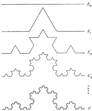
Figure 5. Construction of the von Koch curveF. At each
stage, the middle third of each interval is replaced by the other two sides of an equilateral triangle (Falconer 1990).
Let us see some examples of calculations of the similarity dimension of sets. Figure 5 shows the con-struction of the von Koch curve, and any of its seg-ments of unit length is composed of 4 sub-segseg-ments each of which is scaled down by a factor 1/3 from its parent. Therefore, its similarity dimension is D= log4= log3
= 1:26. This non-integer dimension, greater than one but less than two, reects the prop-erties of the curve. It somehow lls more space than a simple line (D = 1), but less than a Euclidean area of the plane (D = 2). The Figure 5 also shows that the von Koch curve has a nite structure which is reected in irregularities at all scales; nonetheless, this intricate structure stems from a basically simple construction. Whilst it is reasonable to call it a curve, it is too irreg-ular to have tangents in the classical sense. A simple calculation on the von Koch curve shows thatE
k is of length ,
4 3
k
; letting k tend to innity implies that F has innite length. On the other hand,F occupies zero area in the plane, so neither length nor area provides a very useful description of the size ofF.
may regard the dimension as an index of complexity. We can therefore expect that a shape with a high di-mension will be more complicated than another shape with a lower dimension.
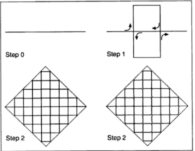
Figure 6. Construction of Peano's plane-lling curve with initiator and generator. In each step the segment is divided in N= 9 parts, each scaled down by= 1=3. This means
the similarity dimension is D = 2. For reasons of clarity
the corners where the curve self-contacts have been slightly rounded (Peitgen, Jurgens and Saupe 1992).
A nice and mathematically fundamental example of this property are the plane-lling curves mentioned above, which we are now in position to discuss in a more quantitative manner. There are many dierent ways of constructing these plane-lling curves and here we shall take the original generator discussed by Peano. Fig-ure 6 shows the construction of the curve and we can see that the generator self-contacts. The gure only shows the rst two stages, but it is obvious that after a few iterations the pattern becomes so complex that pa-per, pencil and our hands turn out to be rather clumsy and inadequate tools to draw the gure, being unable to produce anything with much ner detail than that. Therefore, some sort of computer graphics is then nec-essary to obtain a detailed visualization of such curves. The important aspect of this construction is that the segment is divided inN= 9 parts, each scaled down by = 1=3, which means the similarity dimension of the Peano curve isD= 2.
So we see that this curve has similarity dimension equals to the square, although it is a line which does not self-intersect. The removal of one single point cuts the curve in two pieces which means that its topolog-ical dimension is one. The self-contact points of the
Peano curve are inevitable from a logical and intuitive point of view, and after an innite number of itera-tions we eectively have a way of mapping a part of a plane by means of a topologically one-dimensional curve: given some patch of the plane, there is a curve which meets every point in that patch. The set becomes everywhere dense. The Peano curve is perfectly self-similar, which is shown very clearly in the gure. The generator used to construct the Peano curve is not the only possible one, and in fact there are many dierent ways of constructing such plane-lling curves using dif-ferent generators, although they are generically known as Peano curves. Mandelbrot (1983) shows many dif-ferent and beautiful examples of dierent generators of Peano curves.
I I.3.2 Coastlines
The Hausdor and similarity dimensions dened so far provide denitions of fractal dimension for pure frac-tals, that is, classical fractal sets in a mathematically idealized way. Although some of these classical fractals can be used to model physical structures, what is nec-essary now is to discuss real fractal shapes which are encountered in natural phenomena. Hence, we need to apply as far as possible the mathematical concepts and tools developed so far in the study of real fractal struc-tures, and when the mathematical tools are found to be inadequate or insucient, we need to develop new ones to tackle the problem under study. If the existing tools prove inadequate, it is very likely that a specic denition of fractal dimension appropriate to the prob-lem under consideration will have to be introduced. Let us see next two examples where we actually encounter such situations. The rst is the classical problem of the length of coastlines, where a practical application of the equation (1) gives the necessary tools to charac-terize the shape.
Figure 7. The coast of the southern part of Norway. The gure was traced from an atlas and digitized at about 1800 1200 pixels. The square grid indicated has spacing
of50 km (Feder 1988).
Let us start with the Figure 7 showing the southern part of Norway. The question in this case is: how long is the coast of Norway? On the scale of the map the deep fjords on the western coast show up clearly. The details of the southern part are more dicult to resolve, and if one sails there one nds rocks, islands, bays, faults and gorges that look much the same but do not show up even in detailed maps. This fact is absolutely intuitive and anyone who has walked along a beach and looked at the same beach in the map afterwards can testify it. So before answering the question of how long is the coast under analysis we have to decide on whether the coast of the islands should be included. And what about the rivers? Where does the fjord stop being a fjord and becomes a river? Sometimes this has an easy answer and sometimes not. And what about the tides? Are we discussing the length of the coast at low or high tide?
Despite these initial problems we may press ahead
and try to measure the length of the coast by using an yardstick of length along the coastline of the map, and count the number of stepsN() needed to cover it entirely. If we choose a large yardstick then we would not have to bother about even the deepest fjords, and can estimate the length to beL = N(). However, somebody could raise objections to this measurement based on the unanswered questions above, and we could try a smaller yardstick. This time the large fjords of Figure 7 would contribute to the measured length, but the southeastern coast would still be taken relatively easily in few measurements of the yardstick. Neverthe-less, a serious discussion would demand more detailed maps, which in consequence reveal more details of the coast, meaning that a smaller yardstick is then made necessary. Clearly there is no end to this line of investi-gation and the problem becomes somewhat ridiculous. The coastline is as long as we want to make it. It is a nonrectiable curve and, therefore, length is an inad-equate concept to compare dierent coastlines as this measurement is not objective, that is, it depends on the yardstick chosen.
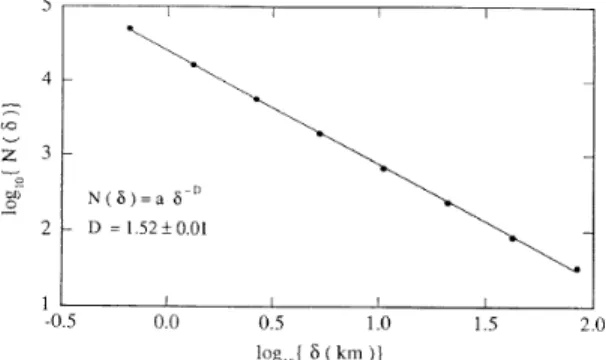
Coasts, which are obviously self-similar on nature, can, nevertheless, be characterized if we use a dierent method based on a practical use of equation (1). In Figure 7 the coast of Norway has been covered with a set of squares with edge length , with the unit of length taken to equal the edge of the frame. Count-ing the number of squares needed to cover the coastline gives the numberN(). If we proceed and ndN() for smaller values of we are able to plot a graph ofN() versus , for dierent grid sizes. Now it follows from equation (1) that asymptotically in the limit of small the following equation is valid:
N()/ 1
D
: (3)
coast. By means of equation (3) we can obtain the expression for the length of coastlines as
L/ 1,D
;
which shows its explicit dependence on the yardstick chosen. The dimensionDin equation (3) is determined by counting the number of boxes needed to cover the set as a function of the box size. It is called box counting dimensionor box dimension.
Figure 8. The number of `boxes' of size needed to cover
the coastline in the previous gure as a function of. The
straight line is a t ofN() /
,D to the observations.
The fractal dimension isD 1:52 (Feder 1988).
The box counting dimension proposes a system-atic measurement which applies to any structure in the plane, and can be readily adapted for structures in the space. It is perhaps the most commonly used method of calculating dimensions and its dominance lies in the easy and automatic computability provided by the method, as it is straightforward to count boxes and maintain statistics allowing dimension calculation. The program can be carried out for shapes with and without self-similarity and, moreover, the objects may be embedded in higher dimensional spaces.
II.3.3 Cluster Dimension
Let us see now the application of fractal ideas to the problem of aggregation of ne particles, such as those of soot, where an appropriate fractal dimension has to be introduced. This kind of application of fractal concepts to real physical systems is under vigorous development at present, inasmuch as it can be used to study such systems even in a laboratory, where they can be grown, or in computer simulations.
The Hausdor dimensionDin equation (1) requires the sizeof the covering sets to vanish, but as physical
systems in general have a characteristic lower length scale, we need to take that into consideration in our physical applications of fractals. For instance, the prob-lem of the length of coastlines necessarily involves a lower cuto in its analysis as below certain scale, say, at the molecular level, we are no longer talking about coastlines. For the same reason we sometimes have to assume upper cutos to the fractal structures we are analysing. This highlights once more an important as-pect of application of fractals to real physical phenom-ena: each problem must be carefully analysed not only to look for the appropriate fractal dimension (or di-mensions as we may have more than one dened in the problem), but also to see to what extent the fractal hypothesis is valid to the case in study.
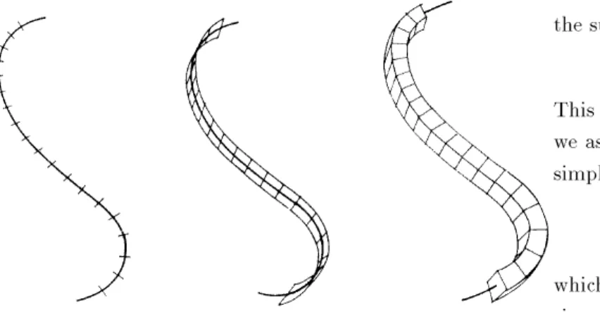
Let us see a specic example. In order to apply the ideas of the previous sections, we can replace a mathematical line by a linear chain of \molecules" or monomers. Figure shows the replacement of a line by a chain of monomers, a two-dimensional set of points by a planar collection of monomers, and a volume by a packing of spheres. Let us call the radiusR
0the small-est length scale of the structure under study. In this case R
0 will be the radius of the monomers in gure . The number of monomers in a chain of length L= 2R is
N =
R R
0
1 :
For a group of monomers in a circular disk we have the proportionality
N /
R R
0
2 :
For the three-dimensional close packing of spherical monomers into a spherical region of radiusR, the num-ber of monomers is
N /
R R
0
3 :
By generalising these relations we may say that the number of particles and the cluster size measured by the smallest sphere of radius Rcontaining the cluster is given by
N /
R R
0
D
; (4)
number-radius relation and D is the cluster fractal di-mensionof the aggregation. The cluster fractal dimen-sion is a measure of how the cluster lls the space it occupies.
Figure 9. Simple aggregation of spherical monomers (Feder 1988).
A fractal cluster has the property of having a de-creasing average density as the cluster size increases, in a way described by the exponent in the number radius relation. The average density will have the form
(R)R 0
,D R
D ,E
; (5)
whereEis the Euclidean dimension of the space where the cluster is placed. Therefore, a cluster is not neces-sarily fractal, even if it is porous or formed at random, as its density may be constant. Note that the shape of the cluster isnotcharacterized by the cluster fractal dimension, although D does characterize, in a quanti-tative way, the cluster's feature of \lling" the space.
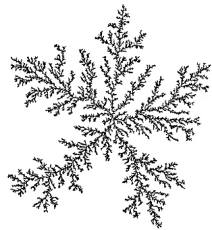
Figure 10 shows a very much studied type of clus-ter, obtained by the diusion-limited aggregation pro-cess (DLA). In this process the cluster is started by a seed in the centre, and wandering monomers stick to the growing cluster when they reach it: if the ran-dom walker contacts the cluster, then it is added to it and another walker is released at a random position on the circle. This type of aggregation process produces clusters that have a fractal dimension D = 1:71 for diusion in the plane. Numerical simulations show that the fractal dimension isD = 2:50 for clusters in three-dimensional space.
Figure 10. Random cluster containing 50,000 particles ob-tained from a two-dimensional diusion-limited aggregation process (DLA) withD = 1:71 (Feder 1988).
Before closing this section, it seems appropriate to discuss something about the limitations of the fractal geometry. For this purpose we shall quote a paragraph from Peitgen, Jurgens and Saupe (1992, p. 244) which beautifully expresses this point.
\The concept of fractal dimension has in-spired scientists to a host of interesting new work and fascinating speculations. Indeed, for a while it seemed as if the fractal dimensions would allow us to discover a new order in the world of complex phenomena and structures. This hope, however, has been dampened by some severe limitations. For one thing, there are several dierent dimensions which give dif-ferent answers. We can also imagine that a structure is a mixture of dierent fractals, each one with a dierent value of box counting di-mension. In such case the conglomerate will have a dimension which is simply the dimension of the component(s) with the largest dimen-sion. That means the resulting number can-not be characteristic for the mixture. What we would really like to have is something more like a spectrum of numbers which gives information about the distribution of fractal dimensions in a structure. This program has, in fact, been carried out and runs under the theme multi-fractals."
For reasons of simplicity we shall not deal with multi-fractals in this paper.
irregular structures on nature, but it does not imply the formulation of a theory for them. Indeed, Mandel-brot has not produced a theory to explain how these structures actually arise from physical laws. A study of the interrelations between fractal geometry and phys-ical phenomena is what may be called the \theory of fractals", and forms the objective of intense activity in the eld nowadays. This activity is basically divided in two main streams. The rst tries to understand how it has come about that many shapes in nature present fractal properties. Hence, the basic question to answer is: where do fractals come from? The second approach is to assume as a matter of fact the existence of fractal structures and to study their physical properties. This generally consists of assuming a simple fractal model as a starting point and studying, for example, some basic physical property, like the diusion on this structure.
As examples of such studies, there are the fractal growth models, which are based on a stochastic growth process in which the probability is dened through Laplace equation (e.g., DLA process). They are con-sidered the prototypes of many physical phenomena that generate fractal structures. As other examples, we have theself-organized critical systems, which are such that a state with critical properties is reached sponta-neously, by means of an irreversible dynamical evolu-tion of a complex system (e.g., sandpile models). They pose problems similarto the fractal growth process, and use theoretical methods inspired by the latter, like the so-called \xed scale transformation", that allows to deal with irreversible dynamics of these process and to calculate analytically the fractal dimension.
I I I.TheFractalHyp othesisfortheDistribution ofGalaxies
In this section we shall discuss how the fractal con-cept can be used to study the large scale distribution of galaxies in the observed universe. We start with a brief summary of the standard methods used to study this distribution. Later we will see the problems of this orthodox analysis and the answers given to these prob-lems when we assume that the large scale distribution of galaxies forms a self-similar fractal system. Some implications of the use of fractal ideas to describe the distribution of galaxies, like a possible crossover to ho-mogeneity, are also presented.
I I I.1 The Standard Correlation Function Ana-lysis
The standard statistical analysis assumes that the objects under discussion (galaxies) can be regarded as point particles that are distributed homogeneously on a suciently large scale. This means that we can mean-ingfully assign an average number density to the distri-bution and, therefore, we can characterize the galaxy distribution in terms of the extent of the departures from uniformityon various scales. The correlation func-tion as introduced in this eld by P. J. E. Peebles around 25 years ago is basically the statistical tool that permits the quantitative study of this departure from homogeneity.
We shall discuss in a moment how to obtain the ex-plicit form of the two-point correlation function, but it is important to point out right now two essential aspects of this method. First that this analysis ts very well in the standard Friedmannian cosmology which assumes
spatial homogeneity, but it does not take into consider-ation any eect due to the curvature of the spacetime. In fact, this method neglects this problem altogether under the assumption that the scales under study are relatively small, although it does not oer an answer to the question of where we need to start worrying about the curvature eects. In other words, this analysis does not tell us what scales can no longer be considered rel-atively small.
Secondly that if the homogeneity assumption is not justied this analysis isinapplicable. Moreover, because this analysis starts by assuming the homogeneity of the distribution,it does not oer any kind of test for the hy-pothesis itself. In other words,this correlation analysis cannot disprove the homogeneous hypothesis.
Let us present now a straightforward discussion on how this statistic can be derived (Raine 1981). If the average number density of galaxies is n=N =V then we have to go on average a distance (n)
,1=3
Specifying this distance in each case is equivalent of giv-ing the locations of all galaxies. This is an awkward way of doing things and does not solve the problem. What we require is a statistical description giving the proba-bility of nding the nearest neighbour galaxy within a certain distance.
However, as the probability of nding a galaxy closer than, say, 50 kpc to the Milky Way is zero, and within a distance greater than this value is one, this is clearly not the sort of probability information we are after; what is necessary is some sort of average. Now we can think that the actual universe is a particular realization of some statistical distribution of galaxies, some statistical law, and the departure from random-ness due to clustering will be represented by the fact that the average value over the statistical ensemble of this separation is less than (n)
,1=3 .
In practice, however, we do not have a statistical ensemble from which the average value can be derived, so what we can do is to take a spatial average over the visible universe, or as much of it as has been cat-alogued, in place of an ensemble average. This only makes sense if the departure from homogeneity occurs on a scale smaller than the depth of the sample, so that the sample will statistically reect the properties of the universe as a whole. In other words, we need to achieve a fair sample of the whole universe in order to fulll this program, and this fair sample ought to be homo-geneous, by assumption. If, for some reason, this fair sample is not achieved, or is not achievable, that is, if the universe has no meaningful average density, this whole program breaks down.
For a completely random but homogeneous distribu-tion of galaxies, the probabilitydP
1of nding a galaxy in an innitesimal volume dV
1 is proportional to dV
1 and to n, and is independent of position. So we have
dP 1= n N dV 1 ;
where N is the total number of galaxies in the sample. The meaning of the probability here is an average over the galaxy sample; the space is divided into volumes dV
1 and we count the ratio of those cells which con-tain a galaxy to the total number. The probability of nding two galaxies in a cell is of order (dV
1) 2
, and so can be ignored in the limitdV
1
!0. It is important to state once more that this procedure only makes sense
if the galaxies are distributed randomly on some scale less than that of the sample.
Suppose now that the galaxies were not clustered. In that case the probability dP
12 of nding galaxies in volumesdV
1 and dV
2 is just the product dP
1 dP
2 of probabilities of nding each of the galaxies, since in a random distribution the positions of galaxies are uncor-related. Now, if the galaxies were correlated we would have a departure from the random distribution and, therefore, the joint probability will dier from a simple product. Thetwo-point correlation function(~r
1 ;~r
2) is by denition a function which determines the dierence from a random distribution. So we put
dP 12= n N 2
[1 +(~r 1
;~r 2)]
dV 1
dV
2 (6)
as the expression of nding a pair of galaxies in vol-umes dV
1, dV
2 at positions ~ r 1,
~ r
2. Obviously, the assumption of randomness on suciently large scales means that (~r
1 ;~r
2) must tend to zero if j~r
1 ,~r
2 j is suciently large. In addition, the assumption of homo-geneity means that cannot depend on the location of the galaxy pair, but only on the distancej~r
1 ,~r
2 jthat separates them, as the probability must be indepen-dent of the location of the rst galaxy. If is positive we have an excess probability over a random distribu-tion and, therefore, clustering. If is negative we have anti-clustering. Obviously >,1. The two-point cor-relation function can be extended to denen-point cor-relation functions, which are functions ofn,1 relative distances, but in practice computations have not been carried out beyond the four-point correlation function. It is common practice to replace the description above using point particles by a continuum description. So if galaxies are thought to be the constituent parts of a uid with variable density n(~r), and if the aver-aging over a volumeV is carried out over scales large compared to the scale of clustering, we have
1 V
Z
V
n(~r)dV = n; (7) wheredV is an element of volume at~r. The joint prob-ability of nding a galaxy indV
1 at ~ r+~r
1 and in dV
2 at~r+~r
2 is given by
1 N
2
n(~r+~r 1)
Averaging this equation over the sample gives
dP
12= 1 N
2 V
Z
V
n(~r+~r 1)
n(~r+~r 2)
dVdV 1
dV 2
: Now if we compare the equation above with equation (6) we obtain
n
2[1 +
(~)] = 1 V
Z
V n(
~ R)n(
~
R+~)dV; (8) where ~ =~r
2 ,~r
1, ~
R=~r+~r 1 and
dV is the volume element at ~
R.
Related to the correlation function is the so-called
power spectrum of the distribution, dened by the Fourier transform of the correlation function. It is also possible to dene anangular correlation functionwhich will express the probability of nding a pair of galaxies separated by a certain angle, and this is the function appropriate to studying catalogues of galaxies which contain only information on the positions of galaxies on the celestial sphere, that is, to studying the projected galactic distribution when the galaxy distances are not available. Further details about these two functions can be found, for instance, in Raine (1981, p. 10). Finally, for the sake of easy comparison with other works it is useful to write equation (8) in a slightly dierent nota-tion:
(r) = hn(~r
0) n(~r
0+ ~ r)i hni
2
,1: (9)
The usual interpretation of the correlation function obtained from the data is as follows. When 1 the system is strongly correlated and for the region when 1 the system has small correlation. From direct calculations from catalogues it was found that at small values ofrthe function(r) can be characterized by a power law (Pietronero 1987; Davis et al. 1988; Geller 1989):
(r)Ar ,
; (1:7); (10) whereAis a constant. This power law behaviour holds for galaxies and clusters of galaxies. The distance r
0 at which = 1 is called the correlation length, and this implies that the system becomes essentially homo-geneous for lengths appreciably larger than this charac-teristic length. This also implies that there should be no appreciable overdensities (superclusters) or under-densities (voids) extending over distances appreciably larger thanr
0.
I I I.2 Dicultiesofthe Standard Analysis The rst puzzling aspect found using the method just described is the dierence in the amplitude A of the observed correlation function (10) when measured for galaxies and clusters of galaxies. While the expo-nent is approximately 1.7 in both cases, for galaxies A
G
' 20 and for clusters A C
' 360. Less ac-curately, superclusters of galaxies were found to have A
SC
' 1000,1500 (see Pietronero 1987 and refer-ences therein). The correlation length was found to be r
0
' 5 h
,1 Mpc for galaxies and r
0
' 25 h
,1 Mpc for clusters.
These are puzzling results, because asA C
' 18A G, clusters appear to be much more correlated than galax-ies, although they are themselves made of galaxies. Similarly superclusters will then appear to be more cor-related than clusters. From the interpretation of (r) described above, the galaxy distribution becomes ho-mogeneous at the distance'10-15 h
,1Mpc where (r) is found to become zero, while clusters and superclus-ters are actually observed at much larger distances, in fact up to the present observational limits.
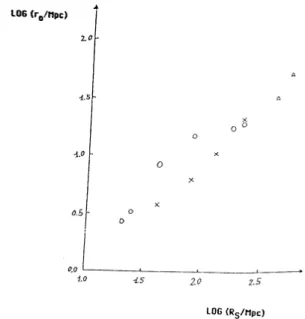
Figure 11. The behaviour ofr0 plotted against the sample
size RS found by Einasto, Klypin and Saar (1986). The
dierent symbols (open circles, crosses and triangles) mean the dierent directions from where the samples were taken in the sky. (Calzetti et al. 1987). Further extensions of this behaviour, to around 100 Mpc, are shown in Pietronero (1997), g. 2.
conrmed by Davis et al. (1988) (see also Calzetti et al. 1987; Coleman, Pietronero and Sanders 1988; Pietro-nero 1997). They found that the correlation length r
0 increases with the sample size. Figure 11 shows this dependence clearly, and it is evident that this result brings into question the notion of a universal galaxy correlation function.
Figure 12. The picture on top shows the observed distri-bution of galaxies in the 18o wide slice centered at 35:5o.
Voids and clusters are clearly visible as well as the lack of homogenization of the sample. The largest inhomogeneities are comparable with the size of the sample and, therefore, it is not large enough to be considered fair. The picture
below shows a sample of 2483 randomly distributed points (Geller 1989).
The third problem of the standard analysis has to do with the homogeneity assumption itself and the pos-sibility of achieving a fair sample, which should not be confused with a homogeneous sample as the standard analysis usually does. A fair sample is one in which there exists enough points from where we are able to derive some unambiguous statistical properties. There-fore homogeneity must be regarded as a property of the sample and not a condition of its statistical validity.
Improvements in astronomical detection techniques, in particular the new sensors and automation, enabled as-tronomers to obtain a large amount of galaxy redshift measurements per night, and made it possible by the mid 1980's to map the distribution of galaxies in three dimensions. The picture that emerged from these sur-veys was far from the expected homogeneity: clusters of galaxies, voids and superclusters appeared in all scales, with no clear homogenization of the distribution. The rst \slice" of the universe shown by de Lapparent, Geller and Huchra (1986) conrmed this inhomogeneity with very clear pictures. More striking is the compari-son of these observed slices with a randomly generated distribution where the lack of homogenizationof the ob-served samples is clear (see Figure 12). Deeper surveys (Saunders et al. 1991) show no sign of any homogeneity being achieved so far, with the same self-similar struc-tures still being identied in the samples.
Those problems together with the power law be-haviour of(r) clearly call for an explanation, and while many have been proposed they usually deal with each of these issues separately. As we shall see, the frac-tal hypothesis, on the other hand, deals with all these problems as a whole and oers an explanation to each of them within the fractal picture. While we do not intend to claim that the fractal hypothesis is the only possi-ble explanation to these propossi-blems, whether considering them together or separately, from now on in this paper we shall take the point of view that fractals oer an attractively simple description of the large scale distri-bution of galaxies and that the model oered by them deserves a deep, serious and unprejudiced investigation, either in a Newtonian or relativistic framework. From its basis, the fractal hypothesis in many ways represents a radical departure from the orthodox traditional view of an observationally homogeneous universe, which is challenged from its very foundations in many respects.
III.3 Correlation Analysis without Assumptions
The method that is going to be introduced obviously does not imply the existence of a fractal distribution, but if it exists, it is able to describe it properly (see Pietronero 1987; Coleman and Pietronero 1992; Pietro-nero, Montuori and Sylos Labini 1997; Sylos Labini, Montuori and Pietronero 1998). The appropriate ana-lysis of pair correlations should therefore be performed using methods that can check homogeneity or fractal properties without assuminga priorieither one. This is not the case of the function(r), which is based on apriori and untested assumption of homogeneity. For this purpose it is useful to start with a basic discussion on the concept of correlation.
If the presence of an object atr
1inuences the prob-ability of nding another object atr
2 these points are said to be correlated. So there is correlation at a dis-tance~rfrom~r
0 if, on average, G(r) =hn(~r
0) n(~r
0+
~r)i6=hni 2
: On the other hand there is no correlation if
G(r)hni 2
:
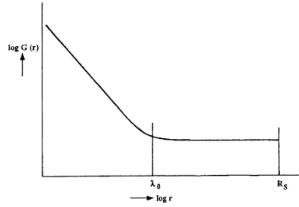
From this it is clear that non-trivial structures like voids or superclusters are made, by denition, from corre-lated points. Hence, the correlation length denition will only be meaningful if it separates correlated regions from uncorrelated ones. Figure 13 shows what would be the typical behaviour we would expect from the galaxy correlation if there is an upper cuto to homogeneity. The power law decay will be eventually followed by a at region that corresponds to the homogeneous dis-tribution. In this case the correlation length
0 is the distance at which there is a change in the correlation G(r): it changes from a power law behaviour to a ho-mogeneous regime and the average density becomes the same, being independent of the position.
Actually in Figure 13 we have a situation where the sample size R
S is larger than
0. If we had R
S <
0, then the average density measured would correspond to an overdensity, dierent from the real average density of the distribution. The precise value of this overdensity would then depend explicitly on the sample radius, and
in this case the function(r) becomes spurious because the normalization of correlated density by the average density (eq. 9) will depend explicitly on R
S. Only in the limiting case where R
S
0 will the length r
0 indeed be related to the correlation length
0
4. This is in fact the case for liquids, where the two-point cor-relation function(r) was originally introduced, as any reasonable sample size larger than some atomic scale for, say, water, will contain so many molecules that its average density is a well dened physical property. Be-cause water has a well dened value forhni, the function (r) will be the same for a glass of water and for a lake, referring only to the physical properties of water and not to the size of the glass. However, by just looking at Figure 12 it is quite clear that this is not the case for the distribution of galaxies. As pointed out by Geller (1989), at least up to the present observational limits the galaxy average density is not well dened.
Figure 13. This illustration represents schematically the expected behaviour for the galaxy correlation density of a correlated system with a crossover to homogeneity. The at behaviour of the functionG(r) beyond some correlation
length
0 corresponds to the unambiguous sign of
homo-geneity (Coleman and Pietronero 1992).
The function G(r) as dened above has, however, the factorhni = N =V which may, in principle, be an explicit function of the sample's size scale. Therefore, it is appropriate to dene the conditional density,(r) as,
,(r) hn(~r
0) n(~r
0+ ~ r)i hni
: (11)
4See
By the denition of the average number density of galaxies, we have
hn(~r 0)
n(~r 0+
~ r)i= 1
V Z
V n(~r
0) n(~r
0+
~r)dV; (12) and together withhni = N =V, equation (11) becomes
,(r) = 1 N
Z
V n(~r
0) n(~r
0+
~r)dV: (13) Assuming
n(~r) = N X
i=1 (~r,~r
i) ; and remembering that
Z +1
,1
(x,y)'(y)dy ='(x); (x) =(,x); equation (13) may be rewritten as
,(r) = 1 N
N X
i=1 n(~r
i+ ~
r) =hn(~r i+
~r)i i
; (14) where n(~r
i + ~
r) is the conditional density of the ith object, and hn(~r
i + ~ r)i
i the nal average that refers to all occupied pointsr
i. This corresponds to assigning an unit mass to all points occupied by galaxies, with the ith galaxy at~r
i and
N being the total number of galaxies. Equation (14) measures the average density at distancerfrom an occupied point, and the volumeV in that equation is purely nominal and should be such to include all objects, but it does not appear explicitly in equation (14). ,(r) is more convenient than G(r) for comparing dierent catalogues since the size of the catalogue only appears via the combination 1
N P
N i=1 and this means that a larger sample volume will only increases the number of objectsN. Hence a larger sam-ple size implies a better statistic.
Equations (9) and (14) are simply related by
(r) = ,( r) hni
,1: (15)
We can also dene theconditional average density ,(
r) = 1 V
Z
V
,(r)dV; (16)
which gives the behaviour of the average density of a sphere of radius r centered around an occupied point averaged over all occupied points 5, and the
integrated
conditionaldensity
I(r) = 4 Z r 0 r 0 2 ,(r 0) dr 0 ; (17)
which is the number of galaxies of a spherical region of radius r.
Figure 14 shows the calculation of ,(r), , (
r) and (r) for the CfA redshift survey, where the absence of a homogenization of the distribution within the sample and the absence of any kind of correlation length are clear. This result brings strong support to the hypoth-esis that the large scale distribution of galaxies forms indeed a fractal system.
Table 1 shows the correlation properties of the galaxy distributions in terms of volume limited cata-logues arising from most of the 50;000 redshift mea-surements that have been made to date. The samples are statistically rather good in relation to the fractal di-mensionD and the conditional density ,(r), and their properties are in agreement with each other.
While various authors consider these catalogs asnot fair, because the contradiction between each other, Pi-etronero, Montuori and Sylos Labini (1997) show that this is due to the inappropriate methods of analysis. Figure 14 shows a density power law decay for many redshift surveys, and it is clear that we have well de-ned fractal correlations from 1 to 1000 h,1 Mpc with fractal dimensionD 2. This implies necessarily that the value ofr
0 ( (r
0) = 1) will scale with sample size R
S,
6which gives the limit of the statistical validity of the sample, as shown also from the specic data about r
0 in table 1. The smaller value of CfA1 was due to its limited size. At this same gure we can see the so-called Hubble-de Vaucouleurs paradox, which is caused by the coexistence between the Hubble law and the frac-tal distribution of luminous matter at the same scales (Pietronero, Montuori and Sylos Labini 1997). 7
5 See Coleman and Pietronero (1992) for a more detailed discussion on this subject with many examples of calculations of ,( r),
,(
r) and(r) using test samples. 6See
xIII.5.1 for an explanation of this eect under a fractal perspective.
Table 1. The volume limited catalogues are characterized by the following parameters: (sr) is the solid angle, R D (h,1 Mpc) is the depth of the catalogue,
R S (h
,1 Mpc) is the radius of the largest sphere that can be contained in the catalogue volume,r
0 (h
,1 Mpc) is the length at which (r
0)
1,D is the fractal dimension and 0 (h
,1 Mpc) is the eventual real crossover to homogeneity that this is actually never observed. The CfA2 and SSRS2 data are not yet available (Pietronero, Montuori and Sylos Labini 1997).
Sample R
D R
S r
0
D
0 CfA1 1.83 80 20 6 1:70:2 >80
CfA2 1.23 130 30 10 2.0 ?
PP 0.9 130 30 10 2:00:1 >130
SSRS2 1.13 150 50 15 2.0 ?
LEDA 4 300 150 45 2:10:2 >150 LCRS 0.12 500 18 6 1:80:2 >500 IRAS 4 80 40 4.5 2:00:1 15 ESP 0.006 700 10 5 1:90:2 >800
Figure 14. ,(r), , (
r) and(r) plotted as function of length
scale for the CfA redshift survey. There is no indication of a homogenization of the sample and both ,(r) and(r) obey a
power law, a result consistent with a fractal structure for the distribution of galaxies. The dashed line indicates a refer-ence slope of,1:7 (Coleman, Pietronero and Sanders 1988).
It is important to mention that there are eects which may conceal the true statistical behaviour of the samples. Those eects may lead to the conclusion that the sample under study is homogeneous, although such a conclusion would be wrong, since such homogeneity may appear not as a statistical property of the sample, but just as an eect of its nite size.
Figure 15. Conditional average density of galaxies plotted as function of distance (decreasing from left to right) for the following redshifts surveys: CfA1 (crosses), Perseus-Pisces (circles) and LEDA (squares). The solid line cor-responds to D = 2. The Hubble redshift-distance is also
shown in this graph. The dotted line corresponds to the Hubble law (increasing from left to right) with H
0 = 55
km s,1 Mpc,1. This law is constructed from: galaxies
with Cepheid-distances forcz>0 (triangles), galaxies with
Tully-Fisher (B-magnitudes) distances (stars), galaxies with SNIa-distances for cz >3000 km/s (lled circles)
(Pietro-nero, Montuori and Sylos Labini 1997).
length V, which is of the order of the mean particle separation, we begin to have signal but this is strongly aected by nite size eects. The correct scaling be-haviour is reached for the region r . In the in-termediate region we have an apparent homogeneous distribution, but it is due to the nite size eects (Pie-tronero, Montuori and Sylos Labini 1997; Sylos Labini, Gabrielli, Montuori and Pietronero 1996; Sylos Labini, Montuori and Pietronero 1998).
As evidence that this new statistical approach is the appropriate method of analysis, we can see in Figure 17 an agreement between various available redshift cata-logues in the range of distances 0:1,110
3h,1Mpc. From this we can conclude that there is no tendency to homogeneity at this scale. In contrast to Figure 17 we have Figure 18 where the traditional analysis based on (r) for the same catalogues of Figure 17 shows a strong conict between these two analytical methods. Figure 18 shows that(r) is unable to say without any doubt if there is a homogeneous scale, and this is the main reason from where the concept of\unfair sample"
is generated.
Figure 16. Schematic behaviour of the density computed from the vertex. Inside the Voronoi's length V (small
dis-tances), one nds almost no galaxies. After this length the number of galaxies starts to grow with a regime strongly aected by nite size uctuations, and the density can be approximately roughly by a constant value, leading to an apparent exponent D3. Finally the scaling regionr
is reached (Pietronero, Montuori and Sylos Labini 1997; Sy-los Labini, Gabrielli, Montuori and Pietronero 1996).
Figure 17. Full correlation for the various redshift cata-logues in the range of distances 0:1,110
3 h,1 Mpc. A
reference line with a slope,1 is also shown (D2). In the
insert it is shown a conic volume. The radial density is com-puted by counting all the galaxies up to a certain limit, and by dividing for the volume of this conic sample (Pietronero, Montuori and Sylos Labini 1997).
Figure 18. Graph of the function (r) versus the distance r(Mpc) for the same galaxy catalogues of Figure 17. Here
we can see rather confusing results generated by thea pri-oriand untested assumption of homogeneity, which are not
present in the real galaxy distribution (Pietronero, Montuori and Sylos Labini 1997).
behaviour of the number counts versus magnitude re-lation (N(< m)) with an exponent = D=5. At small scales = 0:60:1 (D3), which means that we have an apparent homogeneity. However, this is due to the nite size eects discussed above, while at larger scales the value 0:4 (D 2) shows correlation properties of the sample in agreement with the results obtained for ,(r). In addition, the fact that the exponent 0:4 holds up to magnitudes 27,28 seems to indicate that the fractal structure may continue up to 2,310
3 h,1 Mpc (Pietronero, Montuori and Sylos Labini 1997).
I I I.4 Pietronero-Wertz'sSingleFractal (Hierar-chical) Mo del
The single fractal model proposed by Pietronero (1987) is essentially an application of the cluster frac-tal dimension to the large scale distribution of galaxies, a straightforward analysis of the consequences of this fractal interpretation of the galactic system plus the proposal of new statistical tools to analyse the cata-logues of galaxies, derived from his strong criticisms of the standard statistical analysis based on the two-point correlation function. He also studied the problem from a multifractal perspective. What we shall attempt to do here is to present a summary of the basic results re-lated to the discussion above. Later in a review paper, Coleman and Pietronero (1992) extended the theory, with especial emphasis on multifractals and the angu-lar correlation function, and added new results. Further extensions and results of this theory were also made in Sylos Labini, Montuori and Pietronero (1998).
Wertz's (1970, 1971) hierarchical model, on the other hand, was proposed at a time when fractal ideas had not yet appeared. However, these ideas were more or less implicit in his work, and as we shall see below, he ended up proposing a hierarchical model mathemat-ically identical to Pietronero's single fractal model, but 17 years earlier. For this reason his work deserves to be quoted as being the rst independent model where self-similar ideas were applied in the study of the large scale distribution of galaxies. The reasons why Wertz's work was forgotten for so long lies on the shortcomings of its physical implications, as it will be shown below.
Figure 19. The galaxy number counts in the B-band from
several surveys. In the range 12m19 the counts show
an exponent = 0:60:1, while in the range 19m28
the exponent is 0:4. The amplitude of galaxy number
counts form19 (solid line) is computed from the
deter-mination of the prefactorBof the densityn(r) =Br ,(3,D )
at small scale and from the knowledge of the galaxy lumi-nosity function. The distance is computed for a galaxy with
M =,16 and the value used forH
0 is 75 km s
,1 Mpc,1
(Pietronero, Montuori and Sylos Labini 1997).
I I I.4.1 Pietronero'sSingleFractalMo del
there are N 1 = ~
kN
0 objects; in general, within d
n= k
n d
0 (18)
we have
N n= ~
k n
N
0 (19)
objects. Generalizing this idea to a smooth relation, we can dene ageneralized mass-length relationbetweenN and dof the type
N(d) = d D
; (20)
where the fractal dimension
D= log ~ k logk
(21) depends only on the rescaling factors kand ~k, and the prefactor is related to the lower cutos N
0and d
0,
=
N 0 d
0 D
: (22)
Equation (20) corresponds to a continuum limit for the discrete scaling relations.
Figure 20. Schematic illustration of a deterministic fractal system from where a fractal dimension can be derived. The structure is self-similar, repeating itself at dierent scales (Pietronero 1987).
Let us now suppose that a sample of radiusR S con-tains a portion of the fractal structure. If we assume it to be a sphere, then the sample volume is given by
V(R S) = 43
R S
3 ;
which allows us, together with equation (20), to com-pute the average densityhnias being
hni= N(R
S) V(R
S) = 3 4
R S
,
; = 3,D : (23) This is the same type of power law expression obtained several years ago by de Vaucouleurs (1970), and equa-tion (23) shows very clearly that the average density is not a well dened physical property for this sort of fractal system because it is a function of the sample size.
I I I.4.2 Wertz'sHierarchicalMo del
The hierarchical model advanced by Wertz (1970, 1971) was conceived at a time when fractal ideas had not yet appeared. So, in developing his model, Wertz was forced to start with a more conceptual discussion in order to oer \a clarication of what is meant by the `undened notions' which are the basis of any the-ory" (Wertz 1970, p. 3). Then he stated that \a clus-ter consists of an aggregate or gathering ofelements
into a more or less well-dened group which can be to some extent distinguished from its surroundings by its greater density of elements. A hierarchical
struc-ture exists when ith order clusters are themselves
elements of an (i+1)th order cluster. Thus,
galax-ies (zeroth order clusters) are grouped intofirst order cluster. First order clusters are themselves
grouped together to form second order clusters,
etc,ad innitum" (see Figure 21).
Although this sort of discussion may be very well to start with, it demands a precise denition of what one means by a cluster in order to put those ideas on a more solid footing, otherwise the hierarchical structure one is talking about continues to be a somewhat vague notion. Wertz seemed to have realized this diculty when later he added that \to say what percentage of galaxies occur in clusters is beyond the abilities of current observations and involves the rather arbitrary judgment of what sort of grouping is to be called a cluster. (...) It should be pointed out that there is not a clear delineation between clusters and superclusters" (p. 8).
basically a discussion about scaling in the fractal sense, Wertz did develop some more precise notions when he began to discuss specic models for hierarchy, and his starting point was to assume what he called the \univer-sal density-radius relation", that is, the de Vaucouleurs density power law, as a fundamental empirical fact to be taken into account in order to develop a hierarchical cosmology. Then ifM(x;r) is the total mass within a sphere of radius rcentered on the pointx, he dened thevolume density
vas being the average over a sphere of a given volume containingM. Thus
v(
x;r)
3M(x;r) 4 r
3
; (24)
and the global densitywas dened as being
g
lim r !1
v(
x;r): (25)
A pure hierarchyis dened as a model universe which meets the following postulates:
(i)for any positive value ofr in a bounded region, the volume density has a maximum;
(ii) the model is composed of only mass points with nite non-zero mean mass;
(iii)the zero global density postulate: \for a pure hier-archy the global density exists and is zero everywhere" (see Wertz 1970, p. 18).
Figure 21. Reproduction from Wertz (1970, p. 25) of a rough sketch cross-section of a portion of an N=i+ 2 cluster of a
polka dot model.
With this picture in mind, Wertz states that \in any model which involves clustering, there may or may not appear discrete lengths which represent clustering
extreme is the discrete hierarchy in which cluster sizes form a discrete spectrum and the elements of one size cluster are all clusters of the next lowest size" (p. 23). Then in order to describe polka dot models, that is, structures in a discrete hierarchy where the elements of a cluster are all of the same mass and are distributed regularly in the sense of crystal lattice points, it be-comes necessary for one be able to assign some average properties. So if N is the order of a cluster, N = i is a cluster of arbitrary order (gure ), and at least in terms of averages a cluster of mass Mi, diameter Di and com-posed of ni elements, each of mass miand diameter di, has a density given by
i= 6M i Di
3: (26)
From the denitions of discrete hierarchy it is obvious that
Mi,1= ni,1mi,1= mi; (27) and if the ratio of radii of clusters is
ai
Di di
= Di Di,1
; (28)
then thedilution factoris dened as i
i,1
i = ai
3 ni
> 1; (29)
and thethinning rateis given by i
log(i,1=i) log(Di=Di,1) =
log(ai 3=n
i) logai
: (30)
Aregular polka dot modelis dened as the one whose number of elements per cluster ni and the ratio of the radii of successive clusters ai are both constants and independent of i, that is, n and a respectively. Conse-quently, the dilution factor and the thinning rate are both constants in those models,
= a3
n ; = log(a 3=n)
loga : (31)
Thecontinuous representation of the regular polka dot model, which amounts essentially to writing the hierarchical model as a continuous distribution, is ob-tained if we consider r, the radius of spheres centered on the origin, as a continuous variable. Then, from
equation (28) the radius of the elementary point mass r0, is given by
r0= R 1
a ; (32)
where RN is the radius of a Nth order cluster with MN mass, VN volume, and obviously that R0 = r0. It fol-lows from equation (32) the relationship between N and r,
r = aNr
0; (33)
where RN = r.
Notice that by doing this continuous representation Wertz ended up obtaining an equation (eq. 33) which is nothing more than exactly equation (18) of Pietro-nero's single fractal model, although Wertz had reached it by means of a more convoluted reasoning. Actu-ally, the critical hypothesis which makes his polka dot model essentially the same as Pietronero's fractal model was the assumption of regularity of the model because, in this case a and n become constants. Also notice that this continuous representation amounts to chang-ing from discrete to an indenite hierarchy, where in the latter the characteristic length scales for clustering are absent. Therefore, in this representation clusters (and voids) extend to all ranges where the hierarchy is dened, with their sizes extending to all scales be-tween the inner and possible outer limits of the hierar-chy. Hence, in this sense the continuous representation of the regular polka dot model has exactly the same sort of properties as the fractal model discussed by Pi-etronero.
From equation (27) we clearly get MN = n
NM
0; (34)
which is equal to equation (19), except for the dierent notation, and hence the de Vaucouleurs density power law is easily obtained as
v = M N VN
=
3M0 4r0
(logn=loga)
r,; (35) where is the thinning rate
= 3,
logn loga
: (36)