An alternative order parameter for the 4-state potts model

Physica A 366 (2006) 255–264

An alternative order parameter for the 4-state potts model

H.A. Fernandes

, E. Arashiro

, J.R. Drugowich de Felı´cio

, A.A. Caparica

a_{Departamento de Fı´sica e Matema´tica, Faculdade de Filosofia, Cieˆncias e Letras de Ribeira˜o Preto, Universidade de Sa˜o Paulo,} Avenida Bandeirantes, 3900 - CEP 14040-901, Ribeira˜o Preto, Sa˜o Paulo, Brazil

b_{Instituto de Fı´sica, Universidade Federal de Goia´s, C.P. 131, 74.001-970, Goiaˆnia, Goia´s, Brazil}

Received 21 December 2005; received in revised form 21 December 2005 Available online 20 March 2006

Abstract

We have investigated the dynamic critical behavior of the two-dimensional 4-state Potts model using an alternative order parameter first used by Vanderzande [J. Phys. A 20 (1987) L549] in the study of the Z(5) model. We have estimated the global persistence exponentygby following the time evolution of the probabilityPðtÞthat the considered order parameter does not change its sign up to timet. We have also obtained the critical exponentsy,z,n, and busing this alternative definition of the order parameter and our results are in complete agreement with available values found in literature. r2006 Elsevier B.V. All rights reserved.

Keywords:Short-time dynamics; Potts model; Critical phenomena; Monte Carlo methods

1. Introduction

In 1989, Janssen et al.[1]and Huse[2]pointed out, using renormalization group techniques and numerical calculations, respectively, that there is universality and scaling behavior even at an early stage of the time evolution of dynamic systems without conserved order parameter (model A in the terminology of Halperin et al.[3]).

Since then, a great deal of works on phase transitions and critical phenomena using Monte Carlo simulations in the short-time regime have been published and their results are in good agreement with theoretical predictions and numerical results found in equilibrium[4–13]. In addition, the new approach has proven to be useful in determining with good precision the dynamic exponentz, as well as the new exponenty

which governs the so-called critical initial slip [14], the anomalous behavior of the magnetization when the system is quenched to the critical temperatureTc.

The dynamic scaling relation obtained by Janssen et al. [1] for the kth moment of the magnetization, extended to systems of finite size, is written as

MðkÞ_ðt;t;L;m0Þ ¼bkb=nMðkÞðbzt;b1=nt;b1L;bx0m0Þ, (1)

www.elsevier.com/locate/physa

0378-4371/$ - see front matterr2006 Elsevier B.V. All rights reserved. doi:10.1016/j.physa.2006.02.007

_{Corresponding author.}

where t is the time evolution, b is an arbitrary spatial scaling factor, t_{¼ ð}TTcÞ=Tc is the reduced

temperature andLis the linear size of the lattice. The exponentsbandnare as usual the equilibrium critical exponents associated respectively with the order parameter and the correlation length andx0 is related to the

exponentsz,y,bandnby the equation

x0¼yzþb=n. (2)

By setting the scaling factorb_¼t1=z_{andt¼0 in Eq. (1), we obtain the first moment of the magnetization}

M_ðt_Þm0ty, (3)

wherem0 represents the initial magnetization of the system.

Far from equilibrium, another dynamic critical exponent was proposed by Majumdar et al.[15]studying the behavior of the global persistence probabilityP_ðt_Þthat the order parameter has not changed its sign up to the timet. At criticality,P_ðt_Þis expected to decay algebraically as

P_ðt_Þtyg_{, (4)}

whereyg is the global persistence exponent. If the time evolution would be a Markovian process, then the

exponentyg should obey the equation[15]

ygz¼ yzþ d z

b

n. (5)

However, as shown in several works[15–25]the exponentygis an independent critical index closely related to

the non-Markovian character of the process.

In this paper, we estimate the global persistence exponent of the 4-state Potts model employing an alternative order parameter first used by Vanderzande[27]in the study of the Z(5) model. Our estimate is in complete agreement with the results obtained recently for the Ising model with three-spin interactions in one direction and for the 4-state Potts model[26]with its traditional order parameter (see Eq. (8)). In addition, comparing with estimates for the Ising and 3-state Potts models[17], there are consistently increasing values from q_¼2 to 4. In order to check the validity of that alternative order parameter, we also estimate the dynamic critical exponentsyandz, along with the static critical exponentsnandb. Our results [y_¼ 0:046_ð9_Þ,

z_¼2:294_ð3_Þ, n_¼0:669_ð6_Þ, and b_¼0:0830_ð6_Þ] are in complete agreement with previous results found in the literature. In Section 2 we describe the model and the order parameter. In Section 3 we show the short-time scaling relations and present our results. In Section 4 we summarize and conclude.

2. The model

The q-state Potts model [28,29] is a generalization of the Ising model that preserves the next-nearest neighbour interaction, works with only two energies (neighboring spins are in the same state or not) but permits to put at each site any number of states (0pqo1). This model encloses a quite number of other

problems of statistical physics. It undergoes a first-order phase transition whenq44 and a continuous phase transition forqp4. Thus along with the Ising model, the Potts model is an important laboratory to check new

theories and algorithms in the study of critical phenomena. Although its exact solution is not known, several results were obtained during the last 50 years[29–32].

The Hamiltonian of theq-state Potts model is given by

bH_{¼ K}X

hi;ji

dsisj, (6)

whereb_¼1=kBTandkBis the Boltzmann constant,hi;jirepresents nearest-neighbor pairs of lattice sites,Kis

the dimensionless ferromagnetic coupling constant and si is the spin variable which takes the values si¼

0;...;q1 on the lattice sitei. It is well known that the critical point of this model is given by[29]

Usually, the order parameter of this model is given by[4,33]

M1ðtÞ ¼

1

Ld_ðq1Þ X

i

ðqdsiðtÞ;11Þ

* +

, (8)

whereLis the linear size of the lattice andd is the dimension of the system.

In this paper, we use a different definition for the order parameter, first proposed by Vanderzande [27]

studying the Z(5) model. It can be written as

M2ðtÞ ¼

1

Ld X

i

ðdsiðtÞ;0dsiðtÞ;1Þ

* +

, (9)

where the average _{h i}is taken over independent initial configurations.

3. Results

We performed short-time Monte Carlo simulations to obtain the critical exponents for the 4-state Potts model.

Simulations were carried out for square lattices with periodic boundary conditions and dimensionsL_¼120, 180 and 240. We also used the lattice sizesL_¼20, 30, 40, 50, 60 and 90 just to estimate the exponentzthrough the scaling collapses for different lattice sizes. The estimates for each exponent were obtained from five independent bins in the critical temperature. For the exponents yg, z, b andn, each bin consisted of 20 000

samples, whereas for the exponentywe have used 100 000 samples. When estimating the exponentzthrough the scaling collapses, we used 50 000 samples. The error bars are fluctuations of the averages obtained from those bins. The dynamic evolution of the spins is local and updated by the heatbath algorithm.

In the following sections we show the results for the dynamic and static exponents of the 4-state Potts model.

3.1. The dynamic critical exponent yg

First of all we are concerned with the global persistence probabilityP_ðt_Þ. It is defined as the probability that the global order parameter has not changed its sign up to timet. Fort_¼0, the global persistence probability decays algebraically as[15]

P_ðt_Þtyg_{, (10)}

whereyg is the global persistence exponent.

In order to estimate the critical exponentyg, a sharp preparation of the initial states is demanded in order to

obtain a precise value for the initial magnetizationm051. After obtaining the critical exponentyg for several

values of the initial magnetization m0, the final value is achieved from the limitm0!0.

In this moment, it is worth to explain how to obtain a small value ofm0 in Eq. (9). First, each site on the

lattice is occupied by a spin variable which takes the valuess_¼0, 1, 2 or 3 with equal probability. After, the magnetization is measured by using M2ðtÞ and then, the variables in the sites are randomly chosen up to

obtain a null value for the magnetization. The last procedure is to changed sites on the lattice in order to obtain the desired initial magnetization. It is given simply by

m0¼

d

L2 (11)

and a value ofm0 is obtained changingd sites occupied bys¼2 or 3 and substituting them bys¼0.

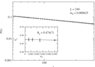
In Fig. 1 we show the behavior of the global persistence probability for L_¼240 and m0¼0:000625 in

double-log scales, together with the behavior of the exponentygform0¼0.005, 0.0025, 0.00125 and 0.000625.

The extrapolated value ofyg, whenm0!0 and L¼240 is

yg¼0:474ð7Þ. (12)

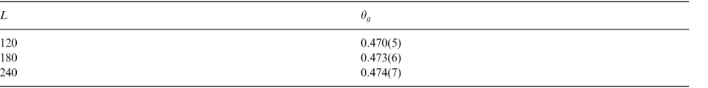
The extrapolated values ofyg forL¼120 and 180 are shown inTable 1. We emphasize that sometimes the

value of the initial magnetizations for the lattice sizeL_¼180 are slightly different from those of theL_¼240. This is necessary in order to obtain an integer value ofd.

The estimates obtained with the three lattice sizes show that the finite size effects are less than the statistical errors. Therefore, we conclude that the values for an infinite lattice are within the error bars of our results for

L_¼240.

3.2. The dynamic critical exponenty

Another critical exponent found only in the nonequilibrium state is the exponenty that characterizes the anomalous behavior of the order parameter in the short-time regime. Formerly, a positive value was always associated to this exponent[4,8,34–38]and the phenomenon was known as critical initial slip. However, some models can exhibit negative values for the exponenty. This is the case, for instance, of the Baxter–Wu model

[5]and the tricritical Ising model, anticipated by Janssen et al.[39]and numerically confirmed by da Silva et al.

[7].

In this paper we reobtain the dynamic critical exponent y for the 4-state Potts model using the order parameter described in Section 2 (Eq. (9)).

Usually the exponenty has been calculated using Eq. (3) or through the autocorrelation

A_ðt_Þtyd=z, (13)

wheredis the dimension of the system. In the present work however we estimated the exponenty using the time correlation of the magnetization[37]

C_ðt_{Þ ¼ h}M_ð0_ÞM_ðt_Þi, (14)

which behaves asty _{whenhMðt¼0Þi ¼0. The average is taken over a set of random initial configurations.}

Initially, this approach had shown to be valid only for models which exhibit up-down symmetry [37]. Nevertheless, it has been demonstrated recently that this approach is more general and can include models with other symmetries[40]. This approach can thus be used for the qa2 Potts models.

100 t 0.001

0.01 0.1

P(t)

0 0.001 0.002 0.003 0.004 0.005 m₀

0.40 0.45 0.50 0.55

θg

θg = 0.474(7)

L = 240 m₀ = 0.000625

When compared to the other two techniques (Eq. (3) and Eq.(13)), this method has at least two advantages. It does not demand a careful preparation of the initial configurations (m051) neither a delicate limitm0!0,

as well as the knowledge in advance of the exponentz(see Eq. (13)), which is an order of magnitude greater thany. In this case, a small relative error inzinduces a large error iny.

InFig. 2we show the time dependence of the time correlationC_ðt_Þin double-log scales for the system with

L_¼240. The linear fit of this curve leads to the value y_¼ 0:046_ð9_Þ.

For the lattice sizes L_¼120 and 180 we obtained respectivelyy_¼ 0:045_ð8_Þand0:046_ð8_Þ. These results are in good agreement with those found for the same model using the order parameter of the Eq. (8)[26,33].

3.3. The dynamic critical exponent z

The critical exponent zwas estimated independently by means of two techniques. We began using mixed initial conditions, in order to obtain the functionF2ðtÞ, given by[41]

F2ðtÞ ¼h

M2_ðt_Þim0¼0

hM_ðt_Þi2_m0¼1 t d=z

, (15)

wheredis the dimension of the system. This approach proved to be very efficient in estimating the exponentz

for a great number of models[5,7,8,19,38,42]. In this technique, for different lattice sizes, the double-log curves ofF2versustfall on the same straight line, without any rescaling of time, resulting in more precise estimates

forz.

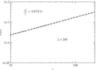
The time evolution ofF2 is shown on log-scales inFig. 3forL¼240.

10 100

t 0.1

0.4 0.7 1

C (t)

L = 240

= -0.046 (9)

Fig. 2. Time correlation of the total magnetization for samples withhMðt¼0Þi ¼0. The error bars were calculated over five sets of 100 000 samples.

Table 1

Global persistence exponentyg

L yg

120 0.470(5)

180 0.473(6)

The slope of the straight line gives

d

z¼0:872ð1Þ, (16)

yielding

z_¼2:294_ð3_Þ. (17)

This result is in good agreement with the valuesz_¼2:294_ð6_Þrecently obtained for the Baxter–Wu model[5],

z_¼2:3_ð1_Þ for the Ising model with multispin interactions [43], and z_¼2:290_ð3_Þ for the 4-state Potts model

[41].

ForL_¼120 we have obtainedz_¼2:296_ð5_Þand forL_¼180 we have obtainedz_¼2:295_ð5_Þindicating that the finite size effects are less than the statistical errors.

The second technique consists of studying the parameter

R_ðT;t;L_{Þ ¼} sign1

L X

top

ðdsiðtÞ;0dsiðtÞ;1Þ

!

sign1

L X

bottom

ðdsiðtÞ;0dsiðtÞ;1Þ

!

* +

(18)

introduced by de Oliveira[44]. In this case, the scaling relation forT_¼Tcis given by[45]

R_ðT _¼Tc;t;L1Þ ¼RðT¼Tc;bzt;bL1Þ, (19)

withb_¼L2=L1. This equation shows that the dynamical exponentzcan be easily estimated by adjusting the

time rescaling factorbzin order to obtain the best scaling collapse of the curves for two different lattice sizes.

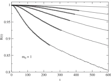
Fig. 4shows the parameter R as a function of the time (full lines), as well as the scaling collapse (open circles) between different pairs of lattice for samples with ordered initial configurations_ðm0 ¼1Þ.

The best values ofz, obtained through thew2_{test [46]for different scaling collapses are shown inTable 2.}

Our results obtained for the collapse ofR_ðt_Þare in good agreement with our results arising fromF2ðtÞ, as

well as the results for the 4-state Potts model [41], and the Baxter–Wu model which belongs to the same universality class[5].

3.4. The static critical exponentsnand b

With the value of the exponentzin hand, we can estimate the static exponentntaking the derivative of the logarithm of the order parameter

M_ðt;t_{Þ ¼}tb=nzM_ð1;t1=nzt_Þ (20)

10 100

t 1e-05

1e-4 1e-3 1e-2

F2

(t)

L = 240 d

z = 0.872(1)

with respect totin the critical point

q_{tlnMðt;tÞjt}

¼0¼t1=nzqt0lnFðt0Þjt0_¼0. (21)

This equation follows a power law that does not depend onLand the functionF_ðt0_{Þis a scaling function which}

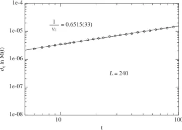
modifies the power law att0a0 but still in the critical domain. In numerical simulations we approximate the derivative by a finite difference. Our results were obtained using finite differences ofKcdwithd¼0:001. In Fig. 5the power law increase of Eq. (21) is plotted in double-log scales forL_¼240.

From the slope of the curve we estimate the exponent 1=nzfor the three lattice sizes. Using the exponentz

calculated previously, we obtain n_¼0:670_ð9_Þ for L_¼120, n_¼0:668_ð6_Þ for L_¼180, and n_¼0:669_ð6_Þ for

L_¼240.

Finally, we evaluate the static exponent bfollowing the decay of the order parameter in initially ordered samples (m0¼1). At the critical temperaturet¼0, the scaling law of Eq. (20) allows one to obtainb=nzwhich

in turn leads to the exponentb, using the previous result obtained for the productnz. InFig. 6we show the time evolution of the magnetization in double-log scale forL_¼240.

A linear fit of this straight line gives the valueb=nz_¼0:0541_ð1_Þleading tob_¼0:0830_ð6_Þ. ForL_¼120 we obtainedb_¼0:0834_ð7_Þand forL_¼180 we obtainedb_¼0:0835_ð4_Þ.

Our results fornandb are in good agreement with the exact resultsn_¼2

3andb¼121 [31,32].

3.5. Anomalous dimension x0

Finally, we calculate the value of the anomalous dimension x0 of the magnetization which is introduced

to describe the dependence of the scaling behavior of the initial conditions. It is related to the exponentsy,z,

0 100 200 300 400 500 600

t 0.8

0.85 0.9 0.95 1

R(t)

m₀ = 1

Fig. 4. RðtÞvstwith ordered initial configurationsm0¼1. The full lines show the behavior ofRðtÞfor latticesL¼20, 30, 40, 50, 60 and 90 (from the bottom to the top) and the corresponding time rescaled curves for latticesL¼30, 40, 50, 60, and 90 (open circles). The exponent zobtained for each collapse is shown inTable 2. The error bars, calculated over five sets of 50 000 samples, are smaller than the symbols.

Table 2

Estimates of the dynamical exponentzfor the best scaling collapse ofRðtÞ

L27!L1 z

30_7!20 2.27(5)

407!30 2.28(4)

50_7!40 2.28(5)

60_7!50 2.29(3)

andb=nby

x0¼yzþb=n. (22)

Table 3shows the values of x0 obtained with the exponents estimated all along this paper.

Our results show that the anomalous dimension of the 4-state Potts model has a null value whose meaning is the presence of the marginal operator, i.e., the operator which has the scaling dimension equal to dimensionality of the system and whose effect is not modified under renormalization-group operations. An

Table 3

The exponentx0for the 4-state Potts model

L x0

120 0:021ð21Þ

180 0:019ð20Þ

240 0:019ð23Þ

10 100

t 1e-08

1e-07 1e-06 1e-05 1e-4

∂τ

ln M(t)

L = 240 1 _{= 0.6515(33)}

Vz

Fig. 5. The time evolution of the derivativeq_tlnMðt;tÞjt¼0on log–log scales in a dynamic process starting from an ordered stateðm0¼1Þ. The error bars are smaller than the symbols. Each point represents an average over five sets of 20 000 samples.

10 100 200

t 0.5

0.7 1.0

M (t)

L = 240

β

= 0.0541(1) Vz

alike value was found recently by Arashiro et al.[26]for this model and for the Ising model with three-spin interactions in one direction.

4. Discussion and conclusions

In this paper we revisited the 4-state Potts model in order to obtain the global persistence exponentygusing

an order parameter first proposed by Vanderzande[27]in the study of the Z(5) model. The results are in good agreement with each other. By using this alternative order parameter, we have also estimated the dynamic critical exponentsyandz, as well as the well-known statical exponentsnandb. The exponentywas estimated using the time correlation of the magnetization, whereas to obtain the exponentzwe used the functionF2ðtÞ

which combines simulations performed with different initial conditions and scaling collapse for the parameter

R introduced by de Oliveira. The statical exponents were obtained through the scaling relations for the magnetization and its derivative with respect to the temperature at Tc. Our results, when compared with

available values in literature support the reliability of this new order parameter.

Acknowledgment

This work was supported by the Brazilian agencies CAPES, FAPESP and FUNAPE-UFG.

References

[1] H.K. Janssen, B. Schaub, B. Schmittmann, Z. Phys. B: Condens. Matter 73 (1989) 539. [2] D.A. Huse, Phys. Rev. B 40 (1989) 304.

[3] B.I. Halperin, P.C. Hohenberg, S.-K. Ma, Phys. Rev. B 10 (1974) 139. [4] B. Zheng, Int. J. Mod. Phys. B 12 (1998) 1419.

[5] E. Arashiro, J.R. Drugowich de Felı´cio, Phys. Rev. E 67 (2003) 046123. [6] K. Okano, L. Schulke, K. Yamagishi, B. Zheng, Nucl. Phys. B 485 (1997) 727. [7] R. da Silva, N.A. Alves, J.R. Drugowich de Felı´cio, Phys. Rev. E 66 (2002) 026130. [8] H.A. Fernandes, J.R. Drugowich de Felı´cio, A.A. Caparica, Phys. Rev. B. 72 (2005) 054434. [9] M. Santos, W. Figueiredo, Phys. Rev. E 63 (2001) 042101.

[10] B.C.S. Grandi, W. Figueiredo, Phys. Rev. E 70 (2004) 056109. [11] M. Pleimling, F. Iglo´i, Phys. Rev. Lett. 92 (2004) 145701. [12] M. Pleimling, F. Iglo´i, Phys. Rev. B 71 (2005) 094424.

[13] A. Malakis, S.S. Martinos, I.A. Hadjiagapiou, Physica A 327 (2003) 349. [14] Z.B. Li, L. Schulke, B. Zheng, Phys. Rev. Lett. 74 (1995) 3396.

[15] S.N. Majumdar, A.J. Bray, S. Cornell, C. Sire, Phys. Rev. Lett. 77 (1996) 3704. [16] S.N. Majumdar, A.J. Bray, Phys. Rev. Lett. 91 (2003) 030602.

[17] L. Schulke, B. Zheng, Phys. Lett. A 233 (1997) 93.

[18] R. da Silva, N.A. Alves, J.R. Drugowich de Felı´cio, Phys. Rev. E 67 (2003) 057102. [19] R. da Silva, N. Alves, Physica A 350 (2005) 263.

[20] F. Ren, B. Zheng, Phys. Lett. A 313 (2003) 312.

[21] E.V. Albano, M.A. Mun˜oz, Phys. Rev. E 63 (2001) 031104. [22] M. Saharay, P. Sen, Physica A 318 (2003) 243.

[23] H. Hinrichsen, H.M. Koduvely, Eur. Phys. J. B 5 (1998) 257. [24] P. Sen, S. Dasgupta, J. Phys. A 37 (2004) 11949.

[25] B. Zheng, Mod. Phys. Lett. B 16 (2002) 775.

[26] E. Arashiro, H. A. Fernandes, J.R. Drugowich de Felı´cio, e-print cond-mat/0603436 (unpublished). [27] C. Vanderzande, J. Phys. A 20 (1987) L549.

[28] R.B. Potts, Proc. Cambridge Phil. Soc. 48 (1952) 106. [29] F.Y. Wu, Rev. Mod. Phys. 54 (1992) 235.

[30] M.P.M. den Nijs, J. Phys. A 12 (1979) 1857.

[31] R.J. Baxter, Exactly Solved Models in Statistical Mechanics, Academic Press, New York, 1982. [32] E. Domany, E.K. Riedel, J. Appl. Phys. 49 (1978) 1315.

[33] R. da Silva, J.R. Drugowich de Felı´cio, Phys. Lett. A 333 (2004) 277. [34] A. Jaster, E. Manville, L. Schulke, B. Zheng, J. Phys. A 32 (1999) 1395. [35] L. Schulke, B. Zheng, Phys. Lett. A 204 (1995) 295.

[37] T. Tome´, M.J. de Oliveira, Phys. Rev. E 58 (1998) 4242.

[38] N. Alves, J.R. Drugowich de Felı´cio, Mod. Phys. Lett. B 17 (2003) 209. [39] H.K. Janssen, K. Oerding, J. Phys. A 27 (1994) 715.

[40] T. Tome´, J. Phys. A 36 (2003) 6683.

[41] R. da Silva, N.A. Alves, J.R. Drugowich de Felı´cio, Phys. Lett. A 298 (2002) 325. [42] R. da Silva, R. Dickman, J.R. Drugowich de Felı´cio, Phys. Rev. E 70 (2001) 067701. [43] C.S. Simo˜es, J.R. Drugowich de Felı´cio, Mod. Phys. Lett. B 15 (2001) 487.

[44] P.M.C. de Oliveira, Europhys. Lett. 20 (1992) 621.

[45] M. Silve´rio Soares, J. Kamphorst Leal da Silva, F.C. Sa´ Barreto, Phys. Rev. B 55 (1997) 1021.