ABSTRACT: Objective: To analyze the conceptual and technical diferences between three deinitions of
spatial relations within a Bayesian mixed-efects framework: classical multilevel deinition, spatial multiple membership deinition and conditional autoregressive deinition with an illustration of the estimate of geographic disparities in early neonatal mortality in Colombia, 2011-2014. Methods: A registry based cross-sectional study was conducted. Births and early neonatal deaths were obtained from the Colombian vital statistics registry for 2011-2014. Crude and adjusted Bayesian mixed efects regressions were performed for each deinition of spatial relation. Model it statistics, spatial autocorrelation of residuals and estimated mortality rates, geographic disparity measures, relative ratios and relative diferences were compared. Results: The deinition of spatial relations between municipalities based on the conditional autoregressive prior showed the best performance according to both it statistics and residual spatial pattern analyses. Spatial multiple membership deinition had a poor performance. Conclusion: Bayesian mixed efects regression with conditional autoregressive prior as an analytical framework may be an important contribution to epidemiological design as an improved alternative to ecological methods in the analyses of geographic disparities of mortality, considering potential ecological bias and spatial model misspeciication.
Keywords: Health status disparities. Early neonatal mortality. Gross domestic product. Vital statistics. Spatial regression. Bayesian analysis.
Comparing deinitions of spatial relations for the
analysis of geographic disparities in mortality
within a Bayesian mixed-efects framework
Comparação de deinições de relações espaciais para a análise das desigualdades
geográicas na mortalidade no quadro de efeitos mistos bayesiana
Diego Fernando Rojas-GualdrónI
IFacultad de Medicina, Universidad CES, Medellín, Antioquia, Colombia.
Corresponding author: Diego Fernando Rojas-Gualdrón. Calle 10 A No. 22 – 04,050021 – Medellín, Antioquia, Colombia. E-mail: [email protected]
INTRODUCTION
In response to growing interest in social and spatial epidemiology studies, which attempt to explain both individual probability of death and between-group disparities within this probability, diferent methodological approaches for area-level data have been proposed in order to simultaneously model them. Many of these proposals are modiications or exten-sions of mixed-efects modeling1. One of the main arguments for its use is the fact that indi-viduals who belong to the same social and geographic group share ecological expositions that make it highly likely that they have similar observed and unobserved characteristics2. Mixed-efects models (MM) have been widely used in public health to model both geograph-ical and non-geographgeograph-ical classiications of people. Some of the most studied classiications are neighborhood and social class, respectively. However, in recent years the applicability and pertinence of hierarchical MM to model geographic data have been discussed. A complete review of the main discussions can be found in a recent paper by Owen et al.3.
In the context of the geographical classiication of people, hierarchical MM captures vertical dependence (hierarchy) but omits horizontal dependence (proximity) between geo-graphic units4. In other words, these models do not take into consideration the spatial con-iguration of geographic units. The validity of interpretations about geographical phenom-ena that arise from non-spatial mixed-efects analyses have been questioned5. Even when the standard hierarchical MM only takes into account individual membership to a single geo-graphic unit, interpretations tend to be done in terms of geogeo-graphical efects. An alternative to standard MM are multiple membership models, which recognize that an individual can
RESUMO:Objetivo: Analisar as diferenças conceptuais e técnicas entre três deinições de relações espaciais dentro do quadro de efeitos mistos bayesiano: deinição multinível clássica, deinição de iliação múltipla espacial e deinição condicional auto regressivo com uma ilustração da estimativa das disparidades geográicas na mortalidade neonatal precoce na Colômbia, 2011-2014. Métodos: Foi realizado um estudo transversal de base do registro. Nascimentos e mortes neonatais precoces foram obtidos a partir do registro de estatísticas vitais Colombiano para o período 2011-2014. Regressões mistas bayesianas brutos e ajustados foram realizadas para cada deinição de relação espacial. As estatísticas de ajuste do modelo, autocorrelação espacial dos resíduos, as estimativas das taxas de mortalidade, as medidas de disparidade geográica, as relações relativas e as diferenças relativas foram comparadas. Resultados:
A deinição das relações espaciais entre os municípios com base no priori condicional auto regressivo apresentou o melhor desempenho de acordo com as estatísticas de ajuste e a análises de padrão espacial dos resíduos. A deinição de iliação múltipla espacial mostrou o mau desempenho. Conclusão: A regressão de efeitos mistos bayesiana com priori condicional auto regressivo como quadro analítico pode ser uma contribuição importante para desenho epidemiológico como uma alternativa melhorada aos métodos ecológicos nas análises das desigualdades geográicas, considerando e potencial viés ecológico e má especiicação do modelo espacial.
belong to multiple groups simultaneously. In a geographical setting, multiple membership is supposed to model the efect of surrounding geographic units on an individual member-ship to a single geographic unit. Nevertheless, membermember-ship models, both single and multi-ple, are closer to the concept of place, which recognizes group membership, but may not operationalize space well, a concept that incorporates the interactions between places6.
Spatial econometricians have also developed techniques to answer similar questions about geographical efects, while public health researchers have mainly opted for multilevel models. One of the most widely used alternatives in spatial econometrics is the simultane-ous autoregressive model (SAR). SAR models7 and other similar ones recognize the spatial arrangement of geographic units but do not allow for the identiication of local diferences. They only permit the evaluation of the global model. In addition, SAR models exclude the possibility of evaluating interactions between the characteristics of individuals and geo-graphic units, which may lead to ecological fallacies.
These two methodological approaches respond to two diferent questions that could become complementary. The hierarchical MM model’s main focus is on vertical depen-dency and vertical efects, while the spatial econometric model’s main focus is on horizontal dependency and horizontal efects. Dong8 identiied how the failure to simultaneously con-sider both efects in research settings, where hierarchical classiication has a spatial nature, may lead to confounding. He found that a hierarchical MM could erroneously treat a hor-izontal interaction efect as a vertical contextual efect; and a spatial econometrics model could erroneously treat a vertical contextual efect as a horizontal interaction efect, which also may lead to confounding. The alternative, to simultaneously consider both efects, are recent. Main developments can be found in spatial econometrics with spatially varying autoregressive models (SVSAR)9, and in public health with spatial random efects models (SREMM)10. SREMM are basically mixed-efects models with spatial consideration deined within a conditional autoregressive prior (CAR). However, those models tend to be applied to aggregate data and have disease mapping purposes rather than analytical purposes with individual data. An exception can be found in recent work by Dong et al. where the model is extended to individual nested data5.
In this paper, a hybrid approach to geographic disparity analyses with elements from social epidemiology and spatial econometrics were tested in an attempt to face spatial relation mis-speciication and ecological bias, the main limitations of each individual methodology. In the context of social and geographic disparities, an appropriate measurement of the magnitude of the between-group variability in mortality, and the identiication of factors that explain it, are highly relevant. They can provide a deeper understanding of the determinants of mortality disparities and consequently, help encourage appropriate public health and policy decisions, which can focus on areas for intervention and the prioritization of resources.
METHODS
DESIGN
A registry based cross-sectional study was conducted. All births recorded in the Vital Statistics registry for the period 2011 – 2014 with complete information on newborn sex, mother’s munic-ipality of residence, and residential area type were considered as part of the study population.
VARIABLES AND DATA SOURCE
Data on births and early neonatal deaths (within irst seven days of life) that occurred during the study period were obtained from the Vital Statistics registry11. 2,666,483 births were recorded, 5,073 (0.2%) birth certiicates had quality problems and were excluded. A total of 2,661,410 births were analyzed. 13,478 early neonatal deaths were registered, 930 (7.0%) death certiicates had quality problems and were excluded. A total of 12,538 deaths were included. Births and deaths were classiied by the mother’s municipality of residence accord-ing to Colombian political-administrative division in 1,122 geographic areas. Residential area type and a proxy of Gross Domestic Product – GDP — were considered as individual and area-level variables, respectively.
DEFINITIONS OF SPATIAL RELATION BETWEEN MUNICIPALITIES
Three Bayesian mixed-efects logistic models of newborns (*i) cross-classiied in munic-ipalities (*(2)) were constructed, one for each deinition of spatial relations. Deinitions are presented in cross-classiied models notation12 to facilitate their comparison. For all models, individual-level early neonatal death, the dependent variable yi, was assumed to be binomi-ally distributed with a probability equal to π
i (Equation 1), and regression equations were deined with a random intercept (β0i) and ixed slopes (βk,k≠0) for individual and area-level variables, as presented in Equation 2.
yi~Binomial (1,π
i) (1)
logit (π
i)= β0i+ β1x1i+ β2x2i +…+ βkxki (2)
autocorrelation (or independence) of area-level residuals and the way to handle them. Only these diferences are highlighted for each deinition. Technical details can be consulted in the references provided.
CLASSICAL MULTILEVEL MODEL (CM)
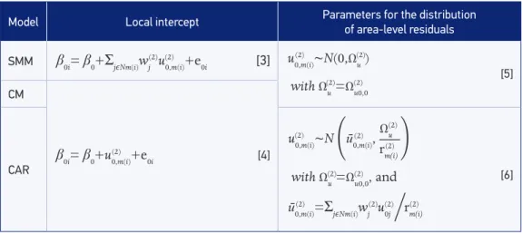
The CM model13 implies a hierarchical structure with no explicit deinition for spatial relations, ignoring the geographic arrangement of municipalities. In this model the esti-mation of residuals (Figure 1, Equation 4) only takes into consideration the municipality where each newborn resides, and independence between area-level residuals is assumed in the distribution function (Figure 1, Equation 5).
SPATIAL MULTIPLE MEMBERSHIP MODEL (SMM)
Similar to the CM model, the SMM model14 assumes independence between area-level residuals in the distribution function, thus it uses the same parameters that the CM model does (Figure 1, Equation 5). However, the spatial dimension is operationalized by weighting the area-level residuals of neighboring municipalities when estimating each local intercept (Figure 1, Equation 3). Consequently, SMM indirectly relates municipalities through the
Model Local intercept Parameters for the distribution
of area-level residuals
SMM β0i= β0+Σj�Nm(i)wj u
0,m(i)+e0i (2)
(2) [3] u
0,m(i)~N(0,Ωu ) (2) (2)
with Ω(2) u =Ω(2) u0,0 [5]
CM
β0i= β0+u0,m(i)+e0i
(2) [4]
CAR
with Ω(2) u =Ωu0,0(2) , and
u(2) 0,m(i)~N �ū0,m(i)(2) ,
(2)
Ωu
(2)
rm(i) � ___
ū0,m(i)=Σj�Nm(i)wj u
0j� (2) (2) (2)
(2) r
m(i)
[6]
β0i: local intercept for the municipality where the newborn i resides; β0: ixed intercept; u0,m(i)
(2) : area-level residual for the
municipality where the newborn i resides; e0i: error term at the individual-level, wj
(2) : area-level weight of the neighbor
municipality j; j Nm� (i): the neighborhood constructed for the municipality where the newborn i resides ; Ω(2)
u: variance of the
area-level residuals; Ω(2)
u0,0: sample variance of the area-level residuals; ū0,m(i): average of the area-level residuals with the
conditional autoregressive prior constrain; r(2)
m(i) : size of the neighborhood of the municipality where the newborn i resides.
Equations are expressed with notation for cross-classiied models12.
cross-classiication of newborns. Neighborhood was deined as all adjacent municipalities and each one was assigned a weight proportional to the size of the neighborhood.
SPATIAL EFFECTS WITH THE CONDITIONAL AUTOREGRESSIVE PRIOR MODEL (CAR)
The CAR model does not assume independence between area-level residuals like the CM and SMM models do. It models area-level spatial autocorrelation of residuals using a conditional autoregressive prior5 with functions for mean and variance, which involve the neighborhoods
residuals (Figure 1, Equation 6). Similar to spatial autocorrelation that is modeled in the distribu-tion funcdistribu-tion, the CAR model does not apply weights to area-level residuals like the SMM model does, but it uses the same equation for the CM model (Figure 1, Equation 4). The CAR model directly relates municipalities at the area-level. The same deinition of neighborhood used for the SMM model was applied to the CAR model, but neighborhoods’ weights were ixed to 1.
For the SMM and CAR models, the neighborhoods’ matrix was constructed with the ArcGIS add-in Adjacency for WinBUGS15.
DATA ANALYSIS
Bayesian estimation speciications
Random models were estimated with second order linearization and empirical Bayes Penalized Quasi-Likelihood methods, as was recommended for modeling spatial data16. A weakly
informa-tive prior with Inverse-Gamma (0.001, 0.001) distribution was used for the variance hyperparam-eter and non-informative priors and normal distribution were used for ixed paramhyperparam-eters based on maximum likelihood estimates. The posterior distributions of parameters were estimated through Markov Chain Monte Carlo Simulations with Gibbs sampling and Metropolis-Hastings updates. Chain convergence was assessed using visual inspection based on graphics of trace, ker-nel density and autocorrelation function. Additionally, efective sample size was expected to be > 200. After a burn-in period of 500 iterations, an additional 5,000 iterations chain was suicient to fulill the requirements for the CM and CAR models but not for the SMM.
The parameters for crude and adjusted spatial relations deinition models with their 95% credible intervals (95%CrI) are presented and compared in terms of proportional reduction (crude parameter– adjusted parameter)/crude parameter.
ESTIMATION OF GEOGRAPHIC DISPARITIES IN MORTALITY
component and are presented as Median Rate Ratio (MRR) and Interquartile Rate Ratio (IqRR). They are two epidemiological measures of heterogeneity proposed by social epidemiology17,18.
ESTIMATION OF RATE RATIOS AND RATE DIFFERENCES FOR INDIVIDUAL AND AREA-LEVEL VARIABLES
Rate Ratios were estimated from regression coeicients. Rate Diferences were estimated from predictions for median diferences against the reference category, and are expressed as deaths per 1,000 LB.
MODEL FIT AND SPATIAL AUTOCORRELATION
Model it was assessed with three it statistics: Deviance Information Criterion (DIC)19, efective number of parameters20 and efective sample size21. The adequacy of the deini-tions of spatial reladeini-tions used to model spatial autocorrelation of area-level residuals was evaluated with Moran’s I statistic. Three spatial patterns on residuals were deined as: clus-tered, over dispersed or not relevant.
Mixed-efects analyses were executed using MLwiN 2.34 (Bristol University, UK). Spatial autocorrelation analyses were executed using ArcMap 10.2.2 (ESRI, US).
ETHICAL CONSIDERATIONS
Approval for this study, protocol number 466/2015, was obtained from the research eth-ics committee of the Universidad CES, Medellin, Colombia.
RESULTS
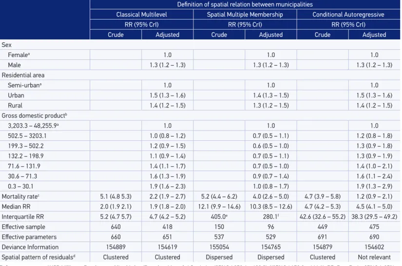
Table 1 shows the estimates of geographic disparities with regard to mortality and rate ratios for individual and area-level variables for each spatial relations deinition model.
ESTIMATION OF GEOGRAPHIC DISPARITIES IN MORTALITY
Table 1. Estimated rate ratios and epidemiological measures of inter-municipal heterogeneity (with 95% credible intervals) for early neonatal mortality according to each spatial relation deinition, Colombia 2011-2014.
Deinition of spatial relation between municipalities
Classical Multilevel Spatial Multiple Membership Conditional Autoregressive
RR (95% CrI) RR (95% CrI) RR (95% CrI)
Crude Adjusted Crude Adjusted Crude Adjusted
Sex
Femalea 1.0 1.0 1.0
Male 1.3 (1.2 – 1.3) 1.3 (1.2 – 1.3) 1.3 (1.2 – 1.3) Residential area
Semi-urbana 1.0 1.0 1.0
Urban 1.5 (1.3 – 1.6) 1.4 (1.3 – 1.5) 1.5 (1.3 – 1.6)
Rural 1.4 (1.2 – 1.5) 1.3 (1.2 – 1.5) 1.4 (1.2 – 1.5)
Gross domestic productb
3,203.3 – 48,255.9a 1.0 1.0 1.0
502.5 – 3203.1 1.0 (0.8 – 1.2) 0.7 (0.5 – 1.1) 1.2 (0.8 – 1.8) 199.3 – 502.2 1.2 (0.9 – 1.5) 0.6 (0.5 – 1.0) 1.3 (0.9 – 1.8) 132.2 – 198.9 1.1 (0.9 – 1.4) 0.7 (0.5 – 1.1) 1.3 (0.9 – 1.9) 71.6 – 131.9 1.4 (1.1 – 1.7) 0.7 (0.5 – 1.0) 1.4 (1.0 – 2.1) 30.6 – 71.3 1.6 (1.3 – 1.9) 0.9 (0.7 – 1.4) 1.6 (1.1 – 2.4) 0.3 – 30.1 1.9 (1.6 – 2.3) 1.0 (0.8 – 1.7) 1.9 (1.3 – 2.9) Mortality ratec 5.1 (4.8 5.3) 2.2 (1.9 – 2.7) 5.2 (4.4 – 6.2) 4.0 (2.6 – 5.0) 4.7 (3.9 – 5.8) 1.2 (0.9 – 2.1) Median RR 2.0 (1.9 2.1) 1.9 (1.8 – 2.0) 12.1 (9.9 – 14.6) 10.3 (8.5 – 12.6) 4.7 (4.2 – 5.3) 4.5 (4.1 – 5.0) Interquartile RR 5.2 (4.7 5.7) 4.7 (4.2 – 5.2) 405.0e 280.1f 42.6 (32.6 – 55.2) 38.3 (29.5 – 49.2)
Efective sample 640 418 150 96 449 475
Efective parameters 660 651 537 529 691 690
Deviance Information 154889 154619 155054 154765 154879 154602 Spatial pattern of residualsd Clustered Clustered Dispersed Dispersed Clustered Not relevant
aReference category; bUSD Millions; cPer thousand live births; dBased on Moran’s I Statistic; e(95%CrI 250.4 – 638.8); f(95%CrI 172.8 – 446.1); RR: Rate Ratio; 95%CrI: 95%
74% respectively. The CAR and SMM models also showed greater uncertainty in credible intervals than the CM model for both crude and adjusted rates.
According to the CAR model crude-MRR, relative diference in mortality is higher than 4.7 for half of the possible comparisons between municipalities. Crude-IqRR shows that for newborns residents of the top 25% highest mortality municipalities, mortality is 42.6 times higher than for newborns residents of the bottom 25% lowest mortality municipali-ties. Crude and adjusted MRR and IqRR were lower for CM than for CAR. Despite these dif-ferences between models, the proportional reduction of the geographic disparity measures after adjustment was similar: 4% for MRR and 10% for IqRR. The SMM model made sub-stantially higher estimations for geographic disparity estimates and for proportional reduc-tion after adjustment, 14% for MRR and 31% for IqRR, compared to both CM and CAR.
ESTIMATION OF RATE RATIOS AND RATE DIFFERENCES FOR INDIVIDUAL AND AREA-LEVEL VARIABLES
The estimates of the individual-level variable Rate Ratios were the same for all models. The estimated relative efect of GDP categories varied between models according to Rate Ratios. Both CM and CAR identiied a social gradient, but classical multilevel median mates were lower and credible intervals were narrower. SMM made an inconsistent esti-mate compared to CM and CAR.
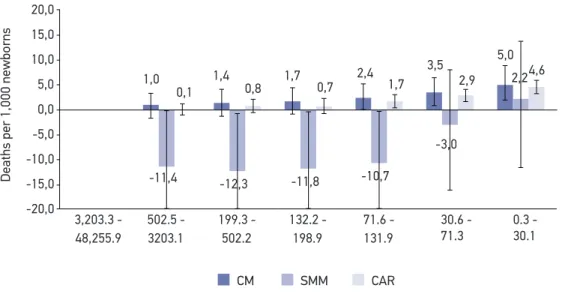
Figure 2 shows the Rate Diferences for municipal GDP categories (reference: 3,203.3 - 48,255.9 USD million). For the area-level variable, the CM estimates were higher than the
Figure 2. Estimated rate diferences (with 95% credible intervals) between the area-level variable gross domestic product according to each spatial relation deinition, Colombia 2011 – 2014.
CM: Classical Multilevel; SMM: Spatial Multiple Membership; CAR: Conditional autoregressive. 48,255.9
3,203.3 - 502.5 -3203.1 199.3 -502.2 132.2 -198.9 71.6 -131.9 30.6 - 71.3 1,0 -3,0 0,1 -20,0 -15,0 -10,0 -5,0 0,0 5,0 10,0 15,0 20,0 D eath s p er 1 ,0 0 0 n ew b or n s
1,4 1,7 2,4 3,5
5,0
-11,4 -12,3 -11,8 -10,7
2,2
0,8 0,7 1,7 2,9
4,6
CM SMM CAR
CAR estimates, and they showed higher uncertainty. According to the median CAR esti-mates, municipalities with a GDP lower than USD 30.1 million have 4.6 more early neo-natal deaths per 1,000 live births than municipalities with a higher GDP. In municipalities with GDP categories USD 30.6 – 71.3 and 71.6 – 131.9 millions, the median rate diference compared to reference category was 2.9 and 1.7 deaths per 1,000 live births. The SMM esti-mates are incoherent with CM and CAR, and show higher uncertainty.
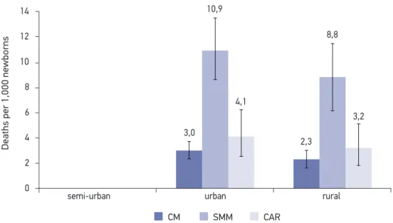
Figure 3 shows the Rate Diferences between newborn’s residential area types (reference: semi-urban). For the individual-level variable, the CAR estimates are higher than the CM, around 1 death per 1,000 live births. The SMM made a considerably higher estimate of Rate Diferences compared to both CAR and CM, and showed higher uncertainty.
MODEL FIT AND SPATIAL AUTOCORRELATION
In terms of model it (Table 1), the CAR model showed the highest number of efective parameters and the lowest DIC for both crude and adjusted models. The CAR also showed the highest efective sample size for the adjusted models, but not between crude models where the CM model showed the highest value. Spatial autocorrelation of area-level resid-uals was properly modeled in the CAR adjusted model, but not in the CAR crude model. Crude and adjusted model patterns of area-level residuals were clustered for CM and dis-persed for SMM.
CM: Classical Multilevel; SMM: Spatial Multiple Membership; CAR: Conditional autoregressive.
Figure 3. Estimated rate diferences (with 95% credible intervals) between the individual-level variable residential area type according to each spatial relation deinition, Colombia 2011-2014.
semi-urban urban rural
3,0 10,9
4,1
2,3 8,8
3,2
0 2 4 6 8 10 12 14
D
e
a
ths
p
er
1,00
0
n
e
wb
o
rn
s
DISCUSSION
The greatest diference between the three deinitions of spatial relations was observed for the area-level variance estimate, which is used to calculate MRR and IqRR—the epide-miological measures of geographic disparity. Diferences can be explained by the spatial autocorrelation of area-level residuals. CM underestimation of geographic disparity may be explained by its lack of a process to model spatially autocorrelated variability. SMM overesti-mated the geographic disparity measures, because when it weighted the residuals (Figure 1, Equation 3), it produced dispersed residuals (beyond what was expected by chance). The CAR estimation of geographic disparity measures can be considered the most appropriate, since its prior for the distribution of residuals (Figure 1, Equation 6) produced spatially non-cor-related residuals and showed the best model it. Additionally, the CAR deinition of spatial relations is a horizontal (proximity) operationalization of space22. The SMM deinition of spatial relations is a vertical (hierarchy) operationalization that does not relate municipali-ties to each other, but rather individuals to multiple municipalimunicipali-ties.
The similarity between the Rate Ratios estimated for sex and residential area type was expected as mixed-models estimates of individual-level ixed efects are intra-cluster spe-ciic, and therefore are not afected by diferences in the estimation of area-level variance23. This is not the case for Rate Diferences estimated for individual-level variables, which were obtained by prediction, a process afected by area-level variance24. A similar logic applies to area-level estimates of Rate Ratios and Rate Diferences, as ixed efects are cluster spe-ciic23. The diferences observed between the CM and CAR models’ GDP Rate Ratios may be explained by the weighting applied to the mean of the normal distribution assumed for the area-level residuals (Figure 1, Equation 6).
Uncertainty diferences in all parameter estimates also must be cautiously interpreted. Even though, in every single case, the CM model produced narrower credible intervals than the CAR, this can be explained by CM underestimation of variance (as explained above). Ignoring autocorrelation leads to spurious certainty25. For the CM model, autocorrelation should be considered when constructing credible intervals. One alternative for maximum likelihood estimation is the method for calculating conidence intervals for Rate Ratios between geographic units in the presence of spatial autocorrelation. This alternative was proposed by Zhu26.
It is important to highlight that even when the CM model showed lower model it than the CAR, and produced spatially auto-correlated residuals, this model cannot be discarded. Two considerations should be made:
1. as said earlier in this paper, the conceptual distinction between place and space must be carefully thought out6. Classical multilevel can be a more adequate model in some research scenarios where group membership is of primary interest rather than spatial distribution;
demographic surveys, or even primary data from complex sampling designs may not be adequate because they do not necessarily have adjacent territories. In those cases, the CM model still can be used, but conclusions must be conined to place interpretations and interpretation of spatial efects should be avoided.
Further research from an epidemiological point of view is needed for a deeper under-standing of those efects in order to clarify the diferential mechanism associated with space and place as geographic dimensions of health. The main hypothesis proposed from these study results is that space and place, as geographic dimensions of health, might behave in a similar fashion as age and cohort do as time dimensions of health, where age-efects may be overlaid by cohort-efects27 leading to confounding. Space-efects may be over-laid by place-efects but more research is needed to test this hypothesis and to provide a structural deinition for bias. Further research from the point of view of biostatistics is also required. It is known28 that for datasets in which low variances are possible, inverse-gamma prior yields an improper posterior distribution for the limit of ε→0, making inferences very sensitive to the values of ε. This is partly due to the complex dependence of the variance marginal likelihood on the distribution of data between area-level units. The CAR model has a more complex variance22 than CM and speciic research on proper priors for it is necessary.
The public health applications of spatial efects models are worth mentioning. Several papers using the deinition of spatial relations with the CAR model can be found for dis-ease mapping and ecological analysis29-32, but their applications and comparisons for geo-graphic disparities research with data at an individual level are scarce33 The main strength of this paper is that the deinitions of spatial relations are performed in a common general framework which makes their comparison more straightforward. Also, diferences in terms of epidemiological measures, estimation, and potential confounding, rather than technical issues, are the main focus.
This study has a number of limitations:
1. The inclusion of the CAR prior was not enough to properly model the spatial nature in the crude model. This is relevant for disease and mortality mapping, since it suggests that even when a proper spatial model is used to represent crude rates distribution with a map, spatial-nonstationarity may not be suiciently modeled. According to indings that were not presented, even when adjusting mortality rates only for sex using the CAR model, the area-level residuals showed no spatial autocorrelation. However, improved model speciication is needed in order to gain a greater understanding of the spatial non-stationarity processes underlying spatial distribution of mortality rates34;
3. Short Markov Chains were used because of the high computational demands of the Bayesian
mixed efect models with the CAR and SMM structures, and few independent variables were considered. However, as the main purpose was to compare diferent deinitions of spatial relation in terms of conceptual and technical aspects, this basic model was enough for illustrative purposes and had enough it evidence and chain stability according to ESS, spatial autocorrelation of residuals, and visual inspection of chain convergence. The persistent spatial autocorrelation of the residuals in CM could be diminished by including more covariates, but it is important to highlight that in spatial data modeling the spatial non-stationarity must not be considered as model misit or noise, but rather as a main process of relevance that should not be adjusted, but rather analytically considered4.
CONCLUSION
The deinition of spatial relations between municipalities based on the conditional autoregressive prior showed the best performance according to both it statistics and spa-tial pattern analyses of area-level residuals. The use of the CAR model in the Bayesian mixed-efects framework, allows for the possibility to simultaneously:
1. estimate individual-level probability of death; 2. estimate mortality rates for geographic units; 3. estimate geographic disparity measures;
4. adjust those estimates for both individual and area-level variables, while properly considering spatial arrangement of the geographic units.
This approach diminishes ecological bias and avoids spatial misspeciication in geographic disparities analyses. If further research increases the validity arguments for this approach, it may be an important contribution to epidemiological design as an alternative to ecolog-ical studies in the study of geographic disparities in mortality.
1. Goldstein H. Multilevel Statistical Models. 4ª ed. New York: Wiley; 2010.
2. Browne W, Goldstein H. MCMC sampling for a multilevel model with non independent residuals within and between cluster units. J Educ Behav Stat. 2010;35(4):453-73.
3. Owen G, Harris R, Jones K. Under examination multilevel models, geography and health research. Prog Hum Geogr. 2015;40(3):394-412.
4. Dong G, Harris R. Spatial autoregressive models for geographically hierarchical data structures. Geogr Anal. 2015;47(2):173-91.
5. Dong G, Ma J, Harris R, Pryce G. Spatial random slope multilevel modeling using multivariate conditional autoregressive models: A case study of subjective travel satisfaction in Beijing. Ann Am Assoc Geogr. 2016;106(1):19-35.
6. Arcaya M, Brewster M, Zigler CM, Subramanian SV. Area variations in health: A spatial multilevel modeling approach. Health Place. 2012;18(4):824-31.
8. Dong G. Simultaneous modelling of contextual and
spatial interaction efects: towards a synthesis of spatial
and multilevel modelling [Doctoral thesis]. [Bristol, U.K.]: University of Bristol; 2014.
9. Mukherjee C, Kasibhatla PS, West M. Spatially varying SAR models and Bayesian inference for high-resolution lattice data. Ann Inst Stat Math. 2014;66(3):473-94.
10. Congdon P. A spatially adaptive conditional autoregressive prior for area health data. Stat Methodol. 2008;5(6):552-63.
11. National Administrative Department of Statistics (CO). Vital statistics database [Internet]. 2012 [cited on 2016 Apr. 7]. Available from: https://www. dane.gov.co/index.php/estadisticas-por-tema/ demograia-y-poblacion/nacimientos-y-defunciones
12. Browne WJ, Goldstein H, Rasbash J. Multiple membership multiple classiication (MMMC) models. Statistical Modelling. 2001;1(2):103-24.
13. Duncan C, Jones K, Moon G. Context, composition and heterogeneity: Using multilevel models in health research. Soc Sci Med 1982. 1998;46(1):97-117.
14. Chandola T, Clarke P, Wiggins RD, Bartley M. Who you live with and where you live: Setting the context for health using multiple membership multilevel models. J Epidemiol Community Health. 2005;59(2):170-5.
15. Upper Midwest Environmental Sciences Center. Adjacency for WinBUGS [Internet]. 2012. [cited 2016 Mar. 14]. Available from: http://www.umesc.usgs.gov/ management/dss/adjacency_tool.html
16. MacNab YC, Lin Y. On empirical Bayes penalized quasi-likelihood inference in GLMMs and in Bayesian disease mapping and ecological modeling. Comput Stat Data Anal. 2009;53(8):2950-67.
17. Merlo J, Chaix B, Ohlsson H, Beckman A, Johnell K, Hjerpe P, et al. A brief conceptual tutorial of multilevel analysis in social epidemiology: Using measures of clustering in multilevel logistic regression to investigate contextual phenomena. J Epidemiol Community Health. 2006;60(4):290-7.
18. Larsen K, Merlo J. Appropriate assessment of neighborhood efects on individual health: integrating random and ixed efects in multilevel logistic regression. Am J Epidemiol. 2005;161(1):81-8.
19. Spiegelhalter DJ, Best NG, Carlin BP, Van Der Linde A. Bayesian measures of model complexity and it. J R Stat Soc Ser B Stat Methodol. 2002;64(4):583-639.
20. Leeuw J de, Meijer E, Eds. Handbook of multilevel analysis. New York: Springer; 2008.
21. Morita S, Thall PF, Müller P. Determining the efective sample size of a parametric prior. Biometrics. 2008;64(2):595-602.
22. Wall MM. A close look at the spatial structure implied by the CAR and SAR models. J Stat Plan Inference. 2004;121(2):311-24.
23. Snijders TAB, Bosker RJ. Multilevel analysis: an introduction to basic and advanced multilevel modeling. 2ª ed. Los Angeles: Sage; 2012.
24. Rasbash J, Charlton C, Jones K, Pillinger R. Manual supplement for MLwiN. Version 2.36 [Internet]. 2016 [cited on 2016 Mar. 14]. Available from: http:// www.bristol.ac.uk/cmm/media/software/mlwin/ downloads/manuals/2-36/supplement-web.pdf
25. Biggs R, Carpenter SR, Brock WA. Spurious Certainty: How Ignoring Measurement Error and Environmental Heterogeneity May Contribute to Environmental Controversies. BioScience. 2009;59(1):65-76.
26. Zhu L, Pickle LW, Pearson JB. Conidence intervals for rate ratios between geographic units. Int J Health Geogr. 2016;15(1):44.
27. Schilling OK. Cohort- and age-related decline in elder’s life satisfaction: is there really a paradox? Eur J Ageing. 2005;2(4):254-63.
28. Gelman A. Prior distributions for variance parameters in hierarchical models (Comment on Article by Browne and Draper). Bayesian Analysis. 2006;1:515-34.
29. Kim H, Sun D, Tsutakawa RK. A bivariate Bayes method for improving the estimates of mortality rates with a twofold conditional autoregressive model. J Am Statistical Assoc. 2001;96(456):1506-21.
30. Neelon B, Anthopolos R, Miranda ML. A spatial bivariate probit model for correlated binary data with application to adverse birth outcomes. Stat Methods Med Res. 2014;23(2):119-33.
31. Por ter AT, Holan SH, Wik le CK. Bayesian semiparametric hierarchical empirical likelihood spatial models. J Statist Plan Inference. 2015;165:78-90.
32. Lee D. A comparison of conditional autoregressive models used in Bayesian disease mapping. Spat Spatio-Temporal Epidemiol. 2011;2(2):79-89.
33. Dasgupta P, Cramb SM, Aitken JF, Turrell G, Baade PD. Comparing multilevel and Bayesian spatial random efects survival models to assess geographical inequalities in colorectal cancer survival: a case study. Int J Health Geogr. 2014;13:36.
34. Fuglstad G-A. Modelling Spatial non-stationarity [Doctoral thesis]. [Trondheim (NO)]: Norwegian University of Science and Technology; 2014.
Received on: 06/05/2016