AbstrAct: The addition of Gurney lap changes the nature of low around airfoil by producing asymmetric Von-Karman vortex in its wake. Most of the investigations on Gurney lapped airfoils have modeled the low using a quasi-steady approach, resulting in time-averaged values with no information on the unsteady features of the low. Among these, some investigations have shown that quasi-steady approach does a good job on predicting the aerodynamic coeficients and physics of low. Previous studies on Gurney lap have shown that the calculated aerodynamic coeficients such as lift and drag coeficients from quasi-steady approach are in good agreement with the time averaged values of these quantities in time accurate computations. However, these investigations were conducted in regimes of medium to high Reynolds numbers where the low is turbulent. Whether this is true for the regime of ultra-low Reynolds number is open to question. Therefore, it is deemed necessary to examine the previous investigations in the regime of ultra-low Reynolds numbers. The unsteady incompressible laminar low over a Gurney lapped airfoil is investigated using three approaches; namely unsteady accurate, unsteady inaccurate, and quasi-steady. Overall, all the simulations showed that at ultra-low Reynolds numbers quasi-steady solution does not necessarily have the same correlation with the time averaged results over the unsteady accurate solution. In addition, it was observed that results of unsteady inaccurate approach with very small time steps can be used to predict time-averaged quantities fairly accurate with less computational cost.
KEYWOrDs: Gurney lap, Ultra-low Reynolds number, NACA 0008 airfoil, Transient behavior, Incompressible low, Laminar low.
Detailed Numerical Study on the
Aerodynamic Behavior of a Gurney Flapped
Airfoil in the Ultra-low Reynolds Regime
Mahzad Khoshlessan1, Seyed Mohammad Hossein Karimian1
INTRODUCTION
Gurney lap (GF) is a tab of small height deployed at the trailing edge of the airfoil normal to the chord line at the pressure side. In the present paper, the efect of diferent numerical approaches on the aerodynamic behavior of a NACA 0008 airfoil equipped with a GF in laminar incompressible low is investigated. GF is a simple device previously used on race cars, which is found to be useful in terms of providing the required downforce. Liebeck (1978) conducted an experimental study of the GF on a Newman airfoil in Douglas Long Beach low-speed wind-tunnel at Reynolds number based on cylinder diameter (ReD) of 3 × 10⁶. The results showed that the GF would provide higher value of maximum lit coeicient (CL), increased lit at a speciic angle of attack, and reduced drag at a speciic CL. he author hypothesized that the low is composed of 2 counter-rotating vortices at the back side of the GF and a recirculating region upstream the lap. Later, this low feature was also observed at low Reynolds number in a water tunnel by Neuhart and Pendergrat (1988).
Li et al. (2002), Myose et al. (1996), and Giguere et al. (1997) studied the efects of GF on the aerodynamic performance of various airfoils. heir results showed that the efect of GF is to substantially increase the maximum CL and to reduce the stall angle. In addition, the zero-lit angle of attack becomes more negative with the increase in GF height. Overall, their results suggest that the efect of the GF is to increase the efective camber of the airfoil. Jefrey et al. (2000) conducted an experimental study
1.Amirkabir University of Technology – Aerospace Engineering Department – Center of Excellence in Computational Aerospace Engineering – Tehran/Iran.
Author for correspondence: Mahzad Khoshlessan | Amirkabir University of Technology – Aerospace Engineering Department – Center of Excellence in Computational Aerospace Engineering | 424, Hafez Ave. | 15875-4413 – Tehran/Iran | Email: [email protected]
over a single-element wing using laser Doppler anemometry along with pressure and force measurements. Based on the study performed by these authors, the time-averaged flow downstream a GF consists of 2 counter-rotating vortices, but the instantaneous low structure actually consists of a wake of alternately shed vortices. Troolin et al. (2006) investigated the wake structure using time-resolved particle image velocimetry. hey showed that 2 distinct vortex-shedding modes exist in the wake. he dominant mode resembles a Karman vortex street behind an asymmetric bluf body. he second mode is caused by the intermittent shedding of recirculating region upstream the lap, which becomes more coherent with the increase in the angle of attack. Manish et al. employed a compressible Reynolds-averaged Navier-Stokes (RANS) solver using Baldwin-Lomax turbulence model for the prediction of flow over NACA 0011 and NACA 4412 airfoils with diferent GF heights. All the computations in their study for NACA 4412 airfoil were performed for free-stream Mach number of 0.20 and chord Reynolds number of 2.0 million; those for NACA 0011 airfoil were carried out for Mach number of 0.14 and chord Reynolds number of 2.2 million.
hey carried out their computations with the assumption that the low is steady. he computed force coeicients had a good correlation with the experiment. But it was observed that the difference between numerical and experimental results increases with angle of attack and flap height. Ashby (1996) conducted experimental and computational studies to investigate the efects of lit-enhancing tabs on a multi-element airfoil. All of the computations were obtained using 2-D, incompressible RANS solver in the steady-state mode implementing the Spalart-Allmaras turbulence model. Good agreement was achieved between computed and experimental results, particularly for cases where no low separation exists on the lap upper surface. However, poor agreement was obtained for conigurations where signiicant low separation exists over the lap upper surface. Overall, the computed results predicted all of the trends observed in the experimental data quite well. Date and Turnock (2002) carried out a detailed computational study on the quasi-steady and periodic performance of NACA 0012 airfoil equipped with GFs with a lap height-to-chord ratio of 2 and 4% using the incompressible RANS solver and implementing the standard k-ε turbulence model at Reynolds number of 0.85 × 10⁶. hey showed that the time-averaged performance is identical to the performance predicted by the quasi-steady solution, showing the same correlation with
the experimental data. According to their investigation, when periodic performance of airfoil is of secondary importance, the quasi-steady solution can be used to obtain estimates of airfoils, mean performance for practical purposes. According to the study performed by Date and Turnock (2002), quasi-steady approach has the same prediction of mean performance as time accurate computations.
Based on the experimental studies in the literature regarding Gurney-flapped airfoils, the addition of flap originates vortex shedding, and the flow becomes unsteady (Jeffrey
et al. 2000; Troolin et al. 2006). As a result, all computations should be performed in unsteady mode. Nevertheless, many numerical computations assume a steady low and use steady- state computations for the prediction of the low (Singh et al.
2007; Ashby 1996; Jang et al. 1992; Ross et al. 1995). To the best of our knowledge, all of the studies in the literature are performed at medium-to-high Reynolds number low regimes. However, less attention has been paid to the performance of GF at ultra-low Reynolds number (Re below 10,000) low regime where the boundary layer, wake characteristics, and other low features are diferent.
lead to steeper take-of ascent, increase in the climb lit-to-drag ratio, and fuel economy (Tejnil 1996). herefore, the choice of an eicient high lit device would also be of great importance. GF is a good candidate to maintain high-lit coeicient required for approach and landing (Storms and Jang 1994) and is a mechanically-simple and cost-efective device in contrast with other complex multi-element high-lit ones, being used to control the low in combination with other elements (Schatz et al. 2004). hus, the motivation for this study was: (a) to model a Gurney-lapped airfoil at ultra-low Reynolds low regime, since the understanding of aerodynamic behavior of the airfoil at this Reynolds number would be helpful for the design of low-speed aircrat; and (b) to investigate whether steady-state solution can still be used to predict mean performance of unsteady low around Gurney-lapped airfoils at ultra-low Reynolds regime. To this end, the Mass Corrected Interpolation Method (MCIM) algorithm of Alisadeghi and Karimian (2010) is employed for the solution of low over a NACA 0008 Gurney-lapped airfoil. his method is one of the most robust ones for incompressible low calculation that provides an eicient and accurate tool for solving practical engineering problems (Alisadeghi and Karimian 2010) and has been previously validated for internal lows (Alisadeghi and Karimian 2010), including Taylor problem, inviscid converging-diverging nozzle, and the lid-driven cavity, as well as for external lows (Khoshlessan
et al. 2013; Khoshlessan 2013), including steady and unsteady lows over a circular cylinder section and unsteady low over a NACA 0012 airfoil.
Three implicit time-marching approaches are imple-mented for the prediction of flow over a Gurney-flapped airfoil: (a) unsteady accurate, which refers to the solution in which linearization iterations are performed at each time step (Δt); (b) unsteady inaccurate, which refers to the solution in which no linearization iteration is performed at each Δt; and (c) quasi-steady, which refers to the solution in which the transient term is eliminated from the Incompressible Navier-Stokes (INS) equations, i.e. very-large time steps are used. Grid reinement and time-step independence studies are conducted to ensure the generation of accurate solution. Results obtained from these approaches are studied in detail and compared with each other. Moreover, the efect of linearization convergence criterion (e) on the time accurate solution and the sensitivity of all calcu-lated parameters to the other values of e are investigated. As it will be seen, the present paper concludes that, in contrast to high Reynolds numbers low, the quasi-steady solution cannot
be used to correctly predict the mean aerodynamic behavior of a Gurney-lapped airfoil at ultra-low Reynolds numbers. It will be also shown that the unsteady inaccurate approach with very-small time steps can be used to fairly predict the time-av-eraged quantities accurately with 1/3 of computational cost needed for unsteady accurate calculations.
In addition, the governing equations are implicitly formulated and solved using direct methods. Two diferent direct solvers are examined here to study their efect on the required memory and speed up of the solution.
NUMERICAL ALGORITHM AND
GOVERNING EQUATIONS
In this study, the MCIM (Alisadeghi and Karimian 2010) is employed for solving 2-D incompressible lows on structured grid systems. he present algorithm can be classiied among the collocated grid schemes in control-volume-based methods in which 2 diferent velocity components at cell faces are deined to suppress the possible checkerboard problem in the solution domain. In the present approach, conservation equations are formed for each control volume throughout the solution domain. In addition, a fully-coupled formulation is used. he linear system of equations obtained in these algorithms is solved using a direct sparse solver. he transient term is modeled using a irst-order backward diference in time. Convective term is linearized by lagging the stream-wise velocity and modeled so that it would cause the upstream value of velocity uup to afect
uip strongly, when convection is dominant. Also, the convective term is modeled using a irst-order backward diferencing in the upstream direction.
convection luxes at the ip should be also related to the nodal values of velocity and pressure.
he volume integral of the transient term is modeled using a first-order backward diference in time. Any integral argument,
i.e.E, F, G, and H, is approximated by its average value over the SCS, which is evaluated at its midpoint location (ip). For difusion flux vectors G and H, bi-linear interpolation is used to directly evaluate the components of stress tensor (Karimian and Schneider 1995, 1994; Karimian 1994). For convective flux vectors E and F, pressure is evaluated using bi-linear interpolation, and the momentum fluxes are linearized with respect to mass fluxes (ρu) and (ρv). Velocity components u and v in mass fluxes are called integration point mass-conserving velocities, being denoted by a hat, i.e.ρu ˆ and ρv ˆ. Other values of u
and v in the momentum fluxes, which are convected by the mass fluxes through the control-volume surface, are called integration point convected velocities. Mass-conserving and convected velocities are cell-face velocities. Details of the modeling of the cell-face velocities are represented in Alisadeghi and Karimian (2010) in detail. It should be noted that, since Navier-Stokes equations are non-linear by nature, and in order to have a linear system of equations, convection terms in momentum equations are linearized by lagging the stream-wise velocity. his means that the mass luxes (ρu and ρv) in convection term are calculated from previous iteration, which introduces an error to the solution. herefore, it is necessary to perform the linearization iteration at each Δt in order to reduce the linearization error to the lowest possible amount. he ε used to stop the linearization iteration process is given by Eqs. 3 and 4, in which zj is the jth unknown variable. For all of the solutions over a circular cylinder shown here, ε is set equal to 0.1%.
t = –1 t = +1
s = –1 s = +1 4 1 2
e.g. scs2
e.g. scs2 3
t
tt
s s
SCV1 SCV4 SCV2 SCV3
Control volume
Sub-control volume Node Element
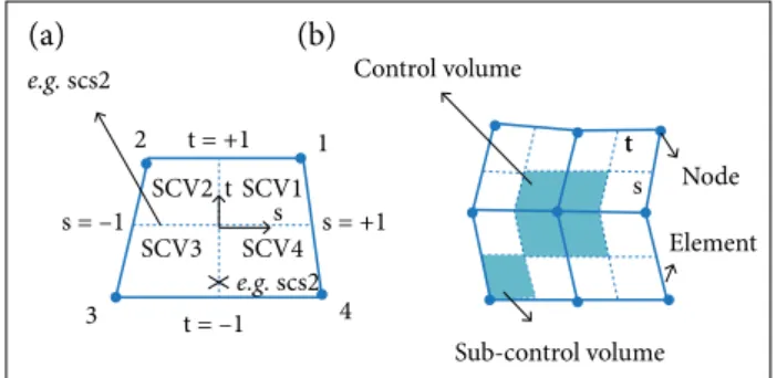
Figure 1. Deinition of (a) element and (b) control volume and sub-control volume.
All primitive variables are located at the vertices of the elements and should be evaluated at the ip to determine the lux at each SCS. Using the linear interpolation, any variable and its gradients within the element can be calculated. More details of the method by which these luxes are deined at the ip and the formation of the system of linearized equations and time-marching scheme can be found in Karimian and Schneider (1995, 1994) and Karimian (1994). Governing equations are the INS equations, and its integral form for SCV2 in Fig. 1, for instance, is given by:
(1)
(3)
(4) (2)
where: dV represents volume differential; dsx and dsy
represent components of the outward vector normal to the surface; SCS denotes the inner sub-control surface associated with SCV2; Q, E, F, G, and H are deined as follows:
where: ρ is the density; u is the convected stream-wise velocity;
v is the convected transverse velocity; μ is the dynamic viscosity.
where:
hree approaches are implemented for all the simulations performed in the present study. Comparison between these approaches are made for the case of Gurney-lapped airfoil. hese approaches are as follows:
• Unsteady accurate solution (UAS), in which linearization iterations are performed at each Δt. he ε used to stop linearization iteration process is deined by Eqs. 3 and 4.
• Unsteady inaccurate solution (UIS), in which no linearization iteration is performed at each Δt.
• Quasi-steady solution (QSS), in which the transient term is eliminated from the INS equations and is considered equivalent to UIS, with Δt → ∞.
bOunDArY cOnDitiOns
Velocity inlet boundary condition is speciied at the inlow boundary, i.e.u = U∞cosα and v = U∞sinα, where U∞is the free stream velocity. Pressure outlet boundary condition is speciied at the outlow boundary, i.e. ∂v/ ∂s = 0 and poutlow= P∞
.
No-slip boundary condition is employed at all walls, i.e. velocities are set equal to 0 on all boundary nodes. GF is considered as a single lat plate without thickness; on its both sides, no-slip boundary condition is applied.iMPLEMEntAtiOn OF bAnD sOLVEr AnD DirEct sPArsE sOLVEr
As mentioned before, in the present numerical study, the governing equations are implicitly formulated, which leads to the formation of a system of linearized equations that should be solved at each Δt (UAS approach). Since the number of unknown variables is typically very large, solving the resulted coeicient matrix has a signiicant impact on computational time. To reduce the amount of required memory and to speed up the convergence rate in the iterative process for the solution of the system of equations, the following tasks and their efects are examined:
• Implementation of band solver.
• Implementation of a direct sparse solver.
he details about the band solver are not given here and can be found in Khoshlessan et al. (2013) and Khoshlessan (2013). Only Sparse solver is discussed, as it is used in all simulations. It should also be noted that all the simulations are executed in serial mode in the present study.
DirEct sPArsE sOLVEr
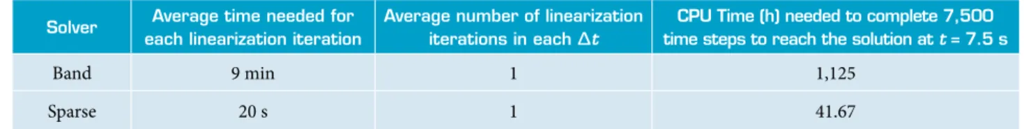
Note that the main part of the present study is dedicated to unsteady lows. herefore, very-ine grids are required to predict time evolution of the wake and the low periodicity. As a result, the number of unknown variables will be very large, which results in a very large coeicient matrix. his leads to a noticeable increase in both CPU time and required memory, especially when extremely intensive computations are necessary to be carried out with small time steps. To handle such cases, a direct sparse solver called BLOCKPACK (Karimian 1994) is implemented instead of the band solver to solve the renumbered band matrix. In order to test the eiciency of the sparse solver, the case of unsteady low over a circular cylinder at ReD= 100 is examined. Table 1 shows the comparison of CPU time taken to complete 7,500 time steps to reach the solution at t = 7.5 s using band solver and direct sparse solver.
As illustrated in Table 1, the average time needed for each linearization iteration is reduced to 20 s for sparse solver as compared to 9 min for band solver. hus, the amount of CPU time taken to complete 7,500 time steps using sparse solver is 1/27 of that of the band solver (41.67/1,125). As can be seen, the implementation of direct sparse solver has led to signiicant speed up in convergence rate and saving in computational time.
ALGORITHM VALIDATION
For the validation of the present algorithm, 2 test cases are studied. In both, cases results are compared against other numerical and experimental results available in the literature (Berthelsen and Faltinsen 2008; Russel and Wang 2003; Linnick and Fasel 2005; Herjord 1996; Calhoun 2002; Medjroubi 2011; Coutanceau and Bouard 1977; Tritton 1959). All the simulations in validation section are performed using the UAS approach. The first test case is steady flow over a circular cylinder at
ReD= 40. Grid reinement study is conducted to ensure that there is enough near wall resolution, and the obtained results are accurate. he numerical grid used for the simulation is an
solver Average time needed for each linearization iteration
Average number of linearization iterations in each Δt
cPu time (h) needed to complete 7,500 time steps to reach the solution at t = 7.5 s
Band 9 min 1 1,125
Sparse 20 s 1 41.67
Table 1. Comparison of CPU time taken to reach periodic state of unsteady low over a circular cylinder at ReD = 100 with
O-type grid topology, composed of quadrilateral elements. he cylinder is located at (x, y) = (D/2, 0), where D is the cylinder diameter. he far-ield boundary is located at 20 chords (C) away from the center of the cylinder in all computations. In this case, grid reinement study is performed based on 2 independent radial (Nr) and angular (Nθ) directions, and the sensitivity of the calculated drag force with change in grid resolution is studied. hree diferent mesh counts with sizes of 220 × 40, 220 × 60, and 220 × 80, in Nr, and with sizes of 180 × 60, 220 × 60, and 260 × 60, in Nθ, are used for this purpose. Drag coeicient (CD) calculated from the steady-state solution and the corresponding relative error (E) on these grids are reported in Tables 2 and 3, which are deined as:
medium grid (220 × 60) is enough tin in the angular direction. herefore, the best grid to obtain grid independent results in this case is the medium one.
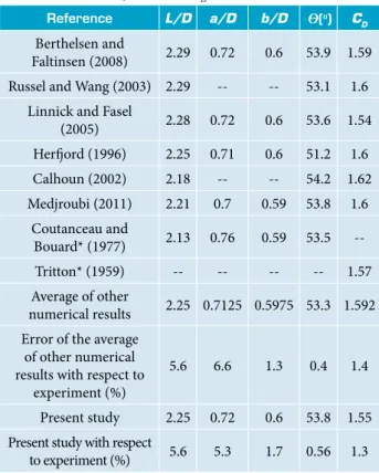
In the next step, the present results are compared with others reported in the literature (Berthelsen and Faltinsen 2008; Russel and Wang 2003; Linnick and Fasel 2005; Herjord 1996; Calhoun 2002; Medjroubi 2011; Coutanceau and Bouard 1977; Tritton 1959). Drag force and geometrical parameters of the steady low structure around a circular cylinder, deined in Fig. 2 and calculated on the 220 × 60 grid, are shown in Table 4, where they are compared with other experimental and numerical
(5)
(6)
Grid Nθ CD Ej,j-1 (%)
1 180 1.5505
--2 220 1.5483 0.1421
3 260 1.5478 0.0323
Table 2. Angular grid independence study at ReD= 40 (N θ = 220).
Grid Nr CD Ej,j-1 (%)
1 40 1.5513
--2 60 1.5505 0.0516
3 80 1.5502 0.0194
Table 3. Angular grid independence study at ReD= 40. (Nr = 60)
In Tables 2 and 3, indices 1, 2, and 3 refer to large, medium, and ine grids used for grid independence study. In Table 2,
E21 and E32 of CDare 0.05 and 0.02, respectively, which are very low. he grid reinement study provides details of ine mesh (220 × 80) compared to medium (220 × 60) and coarse (220 × 40) meshes. Mesh refinement study performed on the coarse, medium, and ine grids on CD shows very little variation when increasing mesh size, leaning towards their limiting trends. herefore, 60 nodes in radial direction would be the best choice here. he irst grid node should be located at 0.00044D away from the cylinder surface for the mesh to be able to capture details of the low ield with this number of grid points. With the same argument, one can conclude that, based on grid reinement study for ine (260 × 60), medium (220 × 60), and coarse (180 × 60) meshes shown in Table 3, the
reference L/D a/D b/D Ѳ(o) C
D
Berthelsen and
Faltinsen (2008) 2.29 0.72 0.6 53.9 1.59
Russel and Wang (2003) 2.29 -- -- 53.1 1.6
Linnick and Fasel
(2005) 2.28 0.72 0.6 53.6 1.54
Herjord (1996) 2.25 0.71 0.6 51.2 1.6
Calhoun (2002) 2.18 -- -- 54.2 1.62
Medjroubi (2011) 2.21 0.7 0.59 53.8 1.6
Coutanceau and
Bouard* (1977) 2.13 0.76 0.59 53.5
--Tritton* (1959) -- -- -- -- 1.57
Average of other
numerical results 2.25 0.7125 0.5975 53.3 1.592
Error of the average of other numerical results with respect to
experiment (%)
5.6 6.6 1.3 0.4 1.4
Present study 2.25 0.72 0.6 53.8 1.55
Present study with respect
to experiment (%) 5.6 5.3 1.7 0.56 1.3 Figure 2. Nomenclature of the geometrical parameters for the low over a circular cylinder at ReD = 40 (Berthelsen and Faltinsen 2008).
Table 4. Comparison of geometrical parameters for the low over a motionless cylinder at ReD = 40.
*Experimental results.
1.5 1 0.5 0
–1 0
θ
1
a/D
L/D
y/D
b/2D
results (Berthelsen and Faltinsen 2008; Russel and Wang 2003; Linnick and Fasel 2005; Herjord 1996; Calhoun 2002; Medjroubi 2011; Coutanceau and Bouard 1977; Tritton 1959). In order to compare the eiciency of the present method concerning other numerical methods, the average of error in other numerical results is calculated. hus, the error of the average of other numerical results as well as the error of the present data, with respect to the experiment (%), are compared. As can be seen, the relative error of the present results for L/D, a/D, b/D, θ/D, and CD are 5.6; 5.3; 1.7; 0.56 and 1.3, respectively, with respect to the experiment, where L is the length of the recirculation region; a is the length of the center of recirculation region; b is the width of the center of recirculation region; θ is the separation angle. hese errors are less than or about the same amount as compared to the relative error in the average of other numerical results, i.e. 5.6; 6.6; 1.3; 0.4 and 1.4 with respect to experiment. hus, it can be concluded that the present algorithm predicts the details of the steady external lows over 2-D bodies very well as compared to other numerical results.
A second test case is performed to validate the present algorithm for the solution of unsteady low that, over a circular cylinder at ReD = 100, at which Von-Karman street is produced in its wake, is used for this purpose. he same grid of 220 × 60 points is adopted for the solution of the unsteady low based on the grid study performed in previous section. his case is solved with diferent time steps to ensure Δt independent solution. During the transient regime, solution linearization iterations are performed at each Δt (refer to Eqs. 3 and 4 for deinition). Solution is continued until the fully periodic state is achieved. Strouhal number(St), mean drag coeicient(CD,m), amplitude drag coeicient(CD,a), and amplitude lit coeicient (CL,a) are extracted from the numerical results obtained from the present solution. Time steps of 10–3; 10–4, and 5 × 10⁻⁵s are considered here, and the corresponding results are shown in Table 5. he change in time step from 10–3 to 10–4s has altered
St, CD,m, CD,a, and CL,a by 1.93; 0.44; 3.25 and 1.12%, respectively, while a decreasing time step from 10–4 to 5 × 10⁻⁵s has changed
St, CD,m, CD,a, and CL,a by only 0.175; 0.004; 0.165 and 0.35%,
respectively. Relative error in the change of parameters listed in Table 5 from time step of 10–4to 5 × 10⁻⁵s are less than 1%. If a relative error of less than 1% is ine enough, then the time step of Δt = 10–4s is an appropriate value to accurately capture unsteady low ield around a circular cylinder at ReD= 100.
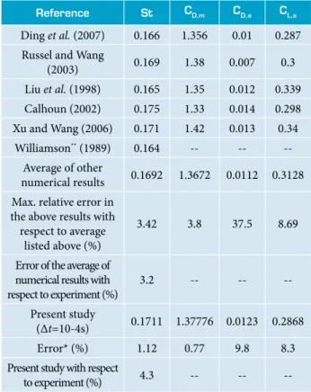
he results are compared with those of the other numerical or experimental studies (Russel and Wang 2003; Calhoun 2002; Ding et al. 2007; Liu et al. 1998; Xu and Wang 2006; Williamson 1989) available in the literature in Table 6. In order to compare the eiciency of the present method as compared to other numerical methods, the average of error in other numerical results is calculated. he maximum relative error of the other numerical results with respect to their average (%) and the error of present data with respect the average of other numerical results
Case Present study St Ej,j-1(%) cD,m Ej,j-1 (%) cD,a Ej,j-1(%) cL,a Ej,j-1 (%)
1 (Δt = 10–3 s) 0.1678 -- 1.372 -- 0.0127 -- 0.2900
--2 (Δt = 10–4s) 0.171 1.93 1.378 0.44 0.0123 3.25 0.2868 1.12
3 (Δt = 5 × 10⁻⁵s) 0.171 0.175 1.378 0.0 0.0121 0.165 0.2858 0.35
Table 5. Time step independence study for unsteady low past circular cylinder at ReD = 100.
reference st cD,m cD,a cL,a
Ding et al. (2007) 0.166 1.356 0.01 0.287
Russel and Wang
(2003) 0.169 1.38 0.007 0.3
Liu et al. (1998) 0.165 1.35 0.012 0.339
Calhoun (2002) 0.175 1.33 0.014 0.298 Xu and Wang (2006) 0.171 1.42 0.013 0.34
Williamson** (1989) 0.164 -- --
--Average of other
numerical results 0.1692 1.3672 0.0112 0.3128
Max. relative error in the above results with respect to average
listed above (%)
3.42 3.8 37.5 8.69
Error of the average of numerical results with respect to experiment (%)
3.2 -- --
--Present study
(Δt=10-4s) 0.1711 1.37776 0.0123 0.2868
Error* (%) 1.12 0.77 9.8 8.3 Present study with respect
to experiment (%) 4.3 -- -- --Table 6. Unsteady low past circular cylinder at ReD=100.
*This is error of the results of the present study (Δt = 10-4 s) with respect to
are compared. As can be seen in Table 6, the relative errors of the present results for St, CD,m, CD,a, and CL,a with respect to the average of other numerical results (Russel and Wang 2003; Calhoun 2002; Ding et al. 2007; Liu et al. 1998; Xu and Wang 2006; Williamson 1989) (1.12; 0.77; 9.8 and 8.3) are less than the maximum relative error in other numerical results (Russel and Wang 2003; Calhoun 2002; Ding et al. 2007; Liu
et al. 1998; Xu and Wang 2006; Williamson 1989) and their average values (3.42; 3.48; 37.5 and 8.69).
Again, from the results obtained here, one can conclude that the present algorithm predicts excellently the details of external unsteady lows over 2-D bodies as well. he relative error of St
for the present results and the average of other numerical results (Russel and Wang 2003; Calhoun 2002; Ding et al. 2007; Liu
et al. 1998; Xu and Wang 2006; Williamson 1989)are 4.3 and 3.2, respectively with respect to experimental data (Table 6). he comparison presented in Table 6 shows that the present algorithm does a good job in predicting the St and aerodynamic coeicients for unsteady low over a circular cylinder.
RESULTS
In this section, the MCIM algorithm of Alisadeghi and Karimian (2010) validated before for external flows over 2-D bodies is used for the analysis of laminar flow over a NACA 0008 airfoil fitted with GF. All of the simulations presented herein are performed by solving the INS equations with the assumption that the flow is laminar over the entire domain. Steady solutions are obtained when aerodynamic forces converge to their final value. Unsteady solutions are obtained after several periodic cycles, where the force coefficient time series reach a periodic state. Grid and time refinement studies are performed to ensure independent solutions. Grid refinement study is first performed in order to find proper number of grid points in different directions of the computational grid. Discussions on grid refinement study are given in the following subsection.
Numerical grid used for the simulation is a structured C-type grid topology. Gurney lapped NACA 0008 airfoil is located at(x,y) = (C/2,0), and the far-ield boundary is located at 20C away from the center of the airfoil in all directions. Uniform flow over the airfoil is from left to the right in the
x-direction, and the entire domain is initialized using the undis- turbed uniform low at the far-ield inlet boundary condition.
GriD rEFinEMEnt stuDY
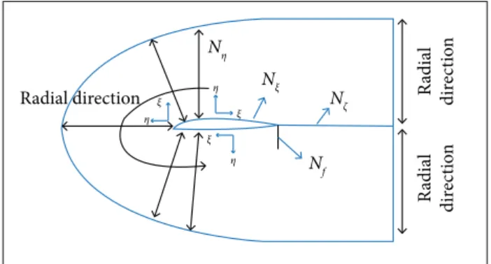
Grid reinement study is conducted on a Gurney lapped airfoil with a lap height of Hf = 4%C, at Reynolds number based on chord length (ReC)of2,000 and angle of attack α = 4°. Grid resolution is changed in diferent regions of computational domain independently, i.e. inside the lap region (Nf), in the radial direction (Nη), along the chord (Nξ), and in the wake (Nζ) to ensure enough grid points in each direction. his will be of great importance to capture physics of the low accurately. Figure 3 shows the schematic diagram of the computational grid around a Gurney lapped airfoil.
R
adi
al
dir
ec
tio
n
R
adi
al
dir
ec
tio
n
Radial direction
η ξ
Nη
Nξ Nζ
Nf
η
η ξ
ξ
Figure 3. Schematic diagram of the computational grid.
It is important to note that the computational time of the unsteady accurate solution approach is much higher than that of the quasi-steady approach, due to the linearization iterations, which should be performed at each Δt in unsteady accurate solution approach. herefore, quasi-steady approach is used in all simulations carried out in this section to avoid the extremely-intensive computational burden due to time accurate computations. hus, the quasi-steady values of lit and drag coeicients are the parameters which their changes due to the grid reinement will be monitored in this study. In each test case, the number of grid points is changed in one direction, while the number of grid points in the other directions is kept constant. Grid reinement study is of great importance in order to reach an independent and accurate solution. Calculated force coeicients along with their relative errors computed on 12 grids with diferent resolutions are considered next. Note that, in the subsequent sections, the error of the lit coeicient (CL) is calculated similarly to error of CD, as deined in Eqs. 3 and 4.
Flap Grid Independence Study
one, and E32 of CD and CLis 0.1353 and 0.0744%, respectively, from the medium grid to the inest one. From the coarsest grid to the inest one, the solution changes, and relative errors of both CD and CL are reduced, leaning toward their limiting trend. herefore, Nf =30 would be the best choice here as the baseline resolution for all subsequent computations.
Wake Grid Independence Study
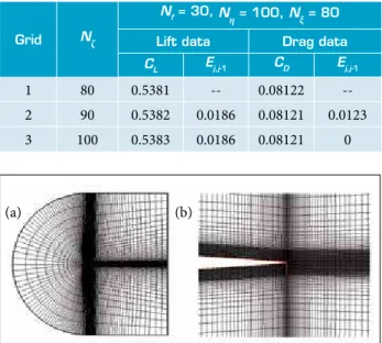
As seen in Table 10, the relative errors of CD and CL are very small. he relative error E32 of CD and CL is approximately 0 and 0.0186% from the medium grid to the inest one, and E21
of CD and CL is approximately 0.0123 and 0.0186% from the coarse grid to the medium one. Based on these data, one can conclude that CD and CLhave reached their limiting values. herefore, the selection of the medium grid with Nζ = 90is an appropriate choice in this case.
Finally, based on the error reduction achieved through grid reinements, a grid with Nf= 30, Nη = 70, Nξ= 100, Nζ = 90 is selected for all the subsequent solutions of Gurney lapped airfoil. his grid is based on the medium cases which yield lit and drag coeicients with very small errors (within 0.2%) from the inest grids. Figure 4a shows the C-grid topology used for the computations, and Fig. 4b presents details of numerical grid used for the simulations in the lap region.
Grid Nf
Nη= 70, Nξ = 100, Nζ= 80
Lift data Drag data
CL Ej,j-1 CD Ej,j-1
1 20 0.5445 -- 0.08092
--2 30 0.5381 1.1894 0.08122 0.3694
3 40 0.5377 0.0744 0.08133 0.1353
Grid Nξ
Nf= 30, Nη = 70, Nζ= 80
Lift data Drag data
CL Ej,j-1 CD Ej,j-1
1 80 0.5371 -- 0.08119
--2 100 0.5381 0.1858 0.08122 0.0369
3 120 0.5389 0.1485 0.08142 0.2456 Table 7. Flap Grid Independence Study with Hf /C = 4% at
ReC = 2,000 and α = 4°.
Radial Grid Independence Study
As seen in Table 8, relative errors of CDand CL are very small. he relative error E32 of CD and CLis approximately 0.012 and 0.074% from the medium grid to the inest one, and E21of CD
and CLis approximately 0.037 and 0.17% from the coarse grid to the medium one. Based on these data, one can conclude that CD and CL have reached their limiting values. herefore,
Nη = 70 would be the best choice here as the baseline resolution for all subsequent computations.
Grid Nη
Nf = 30,N
ξ = 100, Nζ= 80
Lift data Drag data
CL Ej,j-1 CD Ej,j-1
1 60 0.539 -- 0.08119
--2 70 0.5381 0.1673 0.08122 0.0369
3 80 0.5377 0.0744 0.08123 0.0123
Grid Nζ
Nf = 30,N
η = 100, Nξ= 80
Lift data Drag data
CL Ej,j-1 CD Ej,j-1
1 80 0.5381 -- 0.08122
--2 90 0.5382 0.0186 0.08121 0.0123
3 100 0.5383 0.0186 0.08121 0 Table 8. Radial grid independence study with Hf /C = 4% at
ReC = 2,000, and α = 4°.
Chord Wise Grid Independence Study
As can be seen in Table 9, the relative error E32 of CLis approximately 0.1485% from the medium grid to the inest one, and E21of CL is approximately 0.1858% from the coarse grid to the medium one, which shows that CL has reached its limiting value. Regarding the relative error of CD, we believe that, although E32 (0.0002) is larger than E21 (3 × 10⁻⁵), both are small enough to accept that CD has also reached to its limiting value, as can be seen in Table 9. herefore, selection of the medium grid with Nξ = 100 is an appropriate choice in this case.
Table 9. Chord wise grid independence study with Hf /C = 4% at ReC = 2,000, and α = 4°.
Table 10. Wake grid independence study with Hf /C = 4% at
ReC = 2,000, and α = 4°.
Figure 4. Details of computational grid (a) around the section and (b) inside the lap region.
siMuLAtiOns OF FixED GurnEY FLAPPED AirFOiL In the present section, the performance of the quasi-steady approach in comparison with unsteady accurate approach will be evaluated in the regime of ultra-low Reynolds numbers. Diferent approaches for the prediction of low over a Gurney flapped airfoil will be investigated and compared with each other.
Simulations are carried out for a NACA 0008 airfoil with a lap to chord ratioof Hf/C = 4% at angles of attack of 3°, 4°, and 7° and at Reynolds number of 2,000 using the 3 approaches introduced in the section “Implementation of band solver and direct sparse solver”.
Parameters under consideration in the present study are
St, mean lit coeicient (CL,m), CD,m, CL,a, and CD,a, reported in Tables 11 to 13. All the calculated parameters are obtained from CLand CDtime series, once the computed low ield has converged to a periodic solution. he linearization convergence criterion used to stop linearization iteration process for all the calculations summarized in Tables 11 to 13 is ε= 0.1%. To ensure a Δt independent solution for UAS approaches at each angle of attack, variation of St, CL,m, CD,m, CL,a, and CD,a
is monitored for a variety of time steps to achieve accurate
transient solutions for the prediction of unsteady low structure and aerodynamics of a Gurney lapped airfoil.
tiME stEP inDEPEnDEncE stuDY
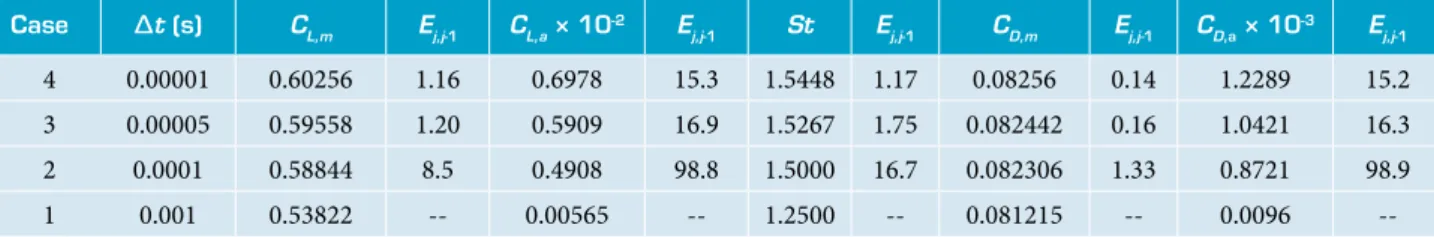
Tables 11 to 13 illustrate the sensitivity of the calculated quantities using UAS approach to diferent time steps ranging from Δt = 10–3s to Δt = 10–5s. As seen in these tables, C
L,m, CD,m, and St extracted from the numerical results calculated using UAS approach show a monotone and asymptotic convergence leaning toward their limiting trend as Δt decreases from
Δt = 10–3 sto Δt = 10–5 s. he relative errors in C
L,m, CD,m, and St from Δt = 10–3 s to Δt = 10–5 s are reduced from 2.59 to 1.37%, 0.33 to 0.15%, and 78.9 to 1.53% at α = 3°; 8.5 to 1.16%, 1.33 to 0.14%, and 16.7 to 1.17% at α = 4°; and 19.03 to 0.74%, 7.75 to 0.23%, and 10.7 to 0.17% at α = 7°, respectively. he
E43 of CL,m, CD,m, and St is 1.37; 0.15 and 1.57% at α = 3°; 1.16; 0.14 and 1.17% at α = 4°; and 0.74; 0.23 and 0.17% at
α = 7°, respectively, which are ine enough and in the same order of magnitude.
Moreover, amplitude lit and drag coeicients extracted from the numerical results of UAS approach also show a monotone and asymptotic convergence as time step decreases from
case Δt (s) CL,m Ej,j-1 CL,a × 10-2 E
j,j-1 St Ej,j-1 CD,m Ej,j-1 CD,a × 10
-3 E
j,j-1
4 0.00001 0.849753 0.74 0.0830 3.37 1.163 0.17 0.114126 0.23 0.02001 3.7
3 0.00005 0.843436 0.95 0.0802 3.9 1.161 0.26 0.113859 0.29 0.01927 4.8
2 0.0001 0.835436 19.03 0.0771 77.04 1.158 10.7 0.113528 7.75 0.01835 79.3
1 0.001 0.676484 -- 0.0177 -- 1.034 -- 0.104730 -- 0.00380
--case Δt (s) CL,m Ej,j-1 CL,a × 10-2 E
j,j-1 St Ej,j-1 CD,m Ej,j-1 CD,a × 10
-3 E
j,j-1
4 0.00001 0.60256 1.16 0.6978 15.3 1.5448 1.17 0.08256 0.14 1.2289 15.2
3 0.00005 0.59558 1.20 0.5909 16.9 1.5267 1.75 0.082442 0.16 1.0421 16.3
2 0.0001 0.58844 8.5 0.4908 98.8 1.5000 16.7 0.082306 1.33 0.8721 98.9
1 0.001 0.53822 -- 0.00565 -- 1.2500 -- 0.081215 -- 0.0096
--case Δt (s) CL,m Ej,j-1 CL,a × 10-2 E
j,j-1 St Ej,j-1 CD,m Ej,j-1 CD,a × 10
-3 E
j,j-1
4 0.00001 0.50659 1.37 0.3215 29.9 1.570 1.53 0.07858 0.15 0.5056 29.6
3 0.00005 0.49963 1.59 0.2253 41.2 1.546 2 0.07846 0.19 0.3561 41.7
2 0.0001 0.49170 2.59 0.1325 99.5 1.515 78.9 0.07832 0.33 0.2075 99.5
1 0.001 0.47897 -- 0.00069 -- 0.319 -- 0.07806 -- 0.001068
--Table 13. Unsteady accurate solution at ReC = 2,000, α = 7° with Hf /C = 4%, ε = 0.1%.
Table 12. Unsteady accurate solution atReC = 2,000, α = 4° with Hf /C = 4%, ε = 0.1%.
Table 11. Unsteady accurate solution at ReC = 2,000, α = 3° with Hf /C = 4%, ε = 0.1%.
Δt = 10–3sto Δt = 10–5s. he relative errors in C
L,a and CD,a
from Δt = 10–3s to Δt = 10–5s is reduced from 99.9 to 29.5% and 99.5 to 29.6% at α = 3°; 98.8 to 15.3% and 98.9 to 15.2% at
α = 4°; and 77.04 to 3.37% and 79.3 to 3.7% at α = 7°, respectively. However, the downward trend is dependent on the angle of attack. For example, E43 of CL,a and CD,a, is 3.37 and 3.7% at α = 7°; 15.3 and 15.2% at α = 4°; 29.9 and 29.6% at α = 3°, respectively. his is due to the fact that values of amplitude force coeicients are 1- or 2-order of magnitude lower than the mean values, i.e.CL,a << CL,m and CD,a<< CD,m. Moreover, the reason for which the relative errors of CL,a and CD,a at
α = 3° are higher than those of α = 4° and the relative errors of CL,a and CD,a at α = 4° are higher than those of α = 7° is that
CL,a at α = 3o<< CL,a at α = 4o<< CL,a at α = 7o and CD,a at α = 3o<< CD,a at α = 4o
<< CD,a at α = 7o.
Based on the data obtained in the Δt independence study shown in Tables 11 to 13, it was decided that a value of 10–5s would be the proper time-step size for the time accurate computations in this Reynolds number. his Δt provides a compromise between accuracy and CPU time. Time steps smaller than Δt = 10–5s would noticeably increase the computational time.
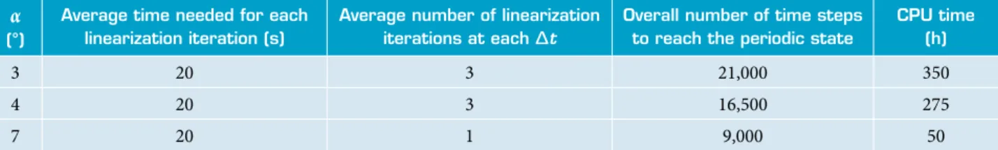
Table 14 shows the comparison of CPU time estimated using UAS approach to reach periodic state with Δt = 10–4s at
ReC= 2,000, with Hf /C = 4%,and ε = 0.1% at diferent angles of attack. he CPU time taken to reach a periodic state is 350, 275, and 50 for 3°, 4°, and 7°, respectively. As can be seen, there is a noticeable diference between the CPU time taken to reach a periodic state, at diferent angles of attack. he computational time at low angles of attack is much higher than that of the large angles of attack. Note that the unsteadiness and amplitude of the oscillation increases as the angle of attack increases. hus, at higher angles of attack, the oscillations dominate uniform low coming from the far-ield boundary in a shorter span of time as compared to lower angles of attack. As a result, for small angles of attack at which the level of unsteadiness is low, forming the vortices and establishing periodic oscillations will take more time as compared to higher angles of attack.
ObsErVAtiOns
One of the main purposes of the present study is to evaluate the possibility of using QSS approach instead of time accurate computations for the prediction of performance. Many numerical studies used the QSS approach for the prediction of low over a Gurney lapped airfoil with the assumption that QSS approach has the capability to predict the low characteristics and the time averaged behavior resulting from time accurate computations with a very good accuracy. Table 15 shows mean lit and drag coeicient errors of QSS approach, i.e. with
Δt = ∞, with respect to UAS approach with Δt = 10–5s. As shown in Table 15, QSS approach has predicted the mean lit and drag coeicients with errors of 5.5 and 0.67%, 10.6 and 1.67% and 35.9 and 14.83%, at α = 3°, 4° and 7°, respectively. As can be seen, the amount of calculated errors is not negligible, and, therefore, QSS approach cannot be used to predict mean lift and drag coefficients with the same accuracy as UAS approach does. In addition, relative errors increase with the angle of attack. For example, the relative error in mean lit and drag coeicients has increased from 5.5 to 35.9% and 0.67 to 14.83%, respectively, by increasing angle of attack from 3° to 7°. his is because the QSS approach introduces the average of low properties instead of details of low transient, while UAS approach presents instantaneous low structure. At higher angles of attack, the low structure is more complicated, and the vortices which are the main cause of unsteadiness are larger. As a result, the error of QSS approach would be higher with respect to UAS approach due to the fact that QSS approach ignores the capture of these vortices of low.
E*(%)
α = 3° α = 4° α = 7°
Δt = ∞
CL,m 5.5 10.6 35.9
CD,m 0.67 1.67 14.83
Table 14. Comparison of CPU time taken to reach periodic state using UAS approach with Δt = 10–4 s for unsteady low over a Gurney lapped NACA 0008 airfoil at ReC = 2,000, with Hf /C = 4%, and ε = 0.1%.
α
(°)
Average time needed for each linearization iteration (s)
Average number of linearization iterations at each Δt
Overall number of time steps to reach the periodic state
cPu time (h)
3 20 3 21,000 350
4 20 3 16,500 275
7 20 1 9,000 50
Table 15. Relative error of quasi-steady approach with respect to unsteady accurate solution (ReC = 2,000, Hf /C = 4%, ε = 0.1%).
In addition, the performance of UIS approach in comparison with that of the UAS approach is also studied. Table 16 shows relative errors of calculated CL,m, CD,m, CL,a, CD,a, and St by UIS approach for 3 time steps of 10–3, 10–5, and 5 × 10⁻⁵s with respect to those calculated by UAS approach with Δt = 10–5 s.
Navier-Stokes equations are non-linear by nature, and, in order to have a linear system of equations, convection terms in momentum equations are linearized with respect to mass luxes
ρu and ρv. herefore, it is necessary to perform the linearization iteration at each Δt in order to reduce the linearization error to the lowest possible amount. As a result, UIS approach in which no linearization iteration is performed does not have the same accuracy as the UAS one.
Table 16 illustrates that, for small time steps, there would be no need to perform linearization iterations. his is reasonable since, when the Δt gets smaller, the error in low properties between 2 successive time steps becomes lower, and, therefore, the
linearization error decreases. For example, with Δt = 5 × 10⁻⁵s, relative errors of calculated CL,m, CL,a, CD,m, CD,a, and St by UIS approach with respect to those calculated by UAS approach are 0.29; 2.02; 0.03; 2.23 and 1.02; 0.29, 0.01, 0.04, 0.2, and 0.89; and 0.31; 1.3; 0.25; 1.4 and 0.79, at α = 3°, 4° and 7°, respectively. As can be seen, all errors are less than or about 2%.
As observed in Table 16, relative errors decrease as Δt
decreases for all parameters studied. For example, relative errors of calculated CL,a by UIS approach with respect to those calculated by UAS approach reduce from 80.7 to 2.02, 15.2 to 0.01, and 5.1 to 1.3 with the decrease in Δt from 1 × 10⁻³s to 5 × 10⁻⁵s at α = 3°, 4° and 7°, respectively. his shows the limiting trend of all parameters with the decrease in Δt from 1 × 10⁻³s to 5 × 10⁻⁵s. Overall, the present results show that UIS approach at small time steps in the order of
Δt = 5 × 10⁻⁵s or lower is comparable with UAS approach and capable of predicting aerodynamic coefficients with a reasonable accuracy.
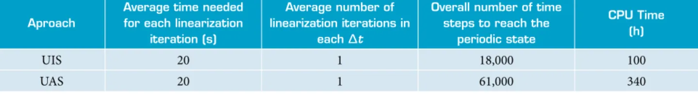
Table 17 shows the comparison of CPU time estimated for the solution to reach its periodic nature using UAS and UIS approaches for the case of unsteady low over a Gurney lapped NACA 0008 airfoil at ReC = 2,000, α = 7°, and Hf/C = 4%.
As illustrated in Table 17, the amount of CPU time taken to solve the flow using the UIS approach (100) is approximately 1/3 of that of UAS approach (340). As can be seen, UIS approach at small time steps is capable of producing time-averaged data with less CPU time than UAS approach. Therefore, using UIS approach with small time steps, such as Δt = 5 × 10⁻⁵s, can lead to savings in computational cost.
EFFEct OF LinEArizAtiOn cOnVErGEncE critEriOn On thE sOLutiOn
The linearization convergence criterion used to stop linearization iteration process was 0.1% in all the simulations presented in the previous sections. In order to ensure that the linearization convergence criterion used to stop linearization iteration process is small enough, simulations of UAS approach are carried out for 3 angles of attack of α = 3°, 4°, and 7° with α (°)
E*(%)
Δt = 0.001 Δt = 0.0001 Δt = 0.00005
3
CL,m 5.3 0.65 0.29
CL,a 80.7 5.1 2.02
CD,m 0.63 0.09 0.03
CD,a 81.01 5.4 2.23
st 20.4 2.5 1.02
4
CL,m 5.3 0.65 0.29
CL,a 15.2 0.54 0.01
CD,m 0.75 0.08 0.04
CD,a 15.4 0.41 0.2
st 19.1 2.4 0.89
7
CL,m 8.6 0.72 0.31
CL,a 5.1 2.5 1.3
CD,m 4.8 0.58 0.25
CD,a 4.4 3.4 1.4
st 16.8 1.92 0.79
Table 16. Errors of unsteady inaccurate solution with respect to unsteady accurate solution (ReC = 2,000, Hf /C = 4%, ε = 0.1%).
*This is the error with respect to Δt = 10-5 s results from unsteady accurate solution.
Aproach
Average time needed for each linearization
iteration (s)
Average number of linearization iterations in
each Δt
Overall number of time steps to reach the
periodic state
cPu time (h)
UIS 20 1 18,000 100
UAS 20 1 61,000 340
Table 17. Comparison of CPU time taken to reach periodic state using UAS (ε = 0.1%, with and Δt = 10–5 s) and UIS
(Δt = 5 × 10⁻⁵ s) for unsteady low over a Gurney lapped NACA 0008 airfoil at Re
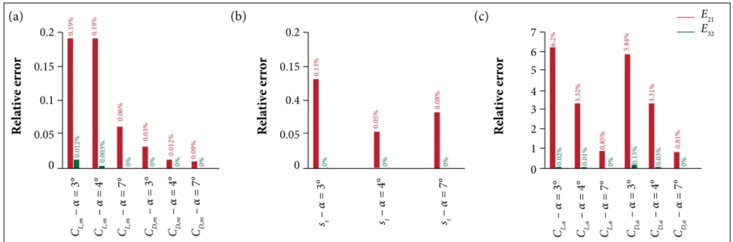
linearization convergence criterion values of ε = 0.1, 0.01, and 0.001% at Δt = 10–5s. he errors indicated in Fig. 5 are deined as:
(7)
(8)
where: indices 1; 2 and 3 refer to the linearization convergence criterion used for each simulation, i.e. ε = 0.1; 0.01 and 0.001%. Note that errors of St, CL,a, CD,m, and CD,aare calculated similarly to the error of CL,m, as deined in Eqs. 7 and 8. Figure 5a shows sensitivity of mean lit and drag coeicients calculated from UAS approach to convergence criterion. he relative errors of E21 of CL,mand CD,mfor 3 angles of attack α = 3°, 4°, and 7° are 0.19; 0.19 and 0.06% as well as 0.03; 0.012 and 0.009%, respectively. he relative errors of E32 of CL,m and CD,m are all very small and approximately zero. As can be seen, mean lit and drag coeicients have negligible changes with linearization convergence criterion and, overall, from ε = 0.1% to ε = 0.01%, their changes are less than 0.2%.
Figure 5b shows sensitivity of Strouhal number calculated from UAS approach to convergence criterion. he relative error of E21
of St for three angles of attack of α= 3°, 4°, 7°, is 0.13; 0.05, and 0.08%, respectively. he relative errors of E32 are 0 for all angles of attack. As observed, the St also has negligible changes with linearization convergence criterion and, overall, its changes are less than 0.2%, similarly to what has been predicted for mean lit and drag coeicients.
Figure 5c shows sensitivity of amplitude lit and drag coeicients calculated from UAS approach to convergence criterion. he
0.06% 0.19% 0.19% 0.03% 0.09% 0.012% 0.012% 0.003% R e la tiv e e rr o r
0% 0% 0% 0%
CL,m – α = 3° CL,m – α = 4° CL,m – α = 7° CD, m – α = 3° CD, m – α = 4° CD, m – α = 7° 0.85% 3.32% 6.2% 5.84% 0.81% 3.31% 0.02% 0.01% R e la tiv e e rr o r
0% 0.15% 0.03% 0%
CL,a – α = 3° CL,a – α = 4° CL,a – α = 7° CD, a – α = 3° CD, a – α = 4° CD, a – α = 7° 0.05% 0.13% 0.08% R e la tiv e e rr o r 0% 0% 0% st – α = 3° st – α = 4° st – α = 7° 0.2 0.15 0.1 0.05 0 1 2 3 4 5 6 7 0 0.2 0.15 0.4 0.05 0 E21 E 32
Figure 5. Linearization convergence criterion independence study at Δt = 10–5 s using UAS for unsteady low over a Gurney lapped NACA 0008 airfoil at ReC = 2,000, with Hf= 4%C, and α = 3°, 4°, and 7°. (a) Mean values of lift and drag coeficients; (b) Strouhal number; (c) Amplitude of lift and drag coeficients.
relative errors of E21 of CL,a and CD,a for 3 angles of attack of α = 3°, 4°, 7°, are 6.2; 3.32; 0.85% and 5.84; 3.31; 0.81%, respectively. he relative errors of E32 of CL,a and CD,a are all very small and approximately zero. As seen amplitude lit and drag coefficients have different behavior from mean lit and drag coeicients and Strouhal number. he changes in relative errors of CL,a and CD,a from ε= 0.1% to ε= 0.01% (E21) are noticeable and dependent on the angle of attack. As seen in Fig. 5c, the relative errors of E21 of CL,a and CD,a
decreases when the angle of attack increases. Indeed, amplitude lit and drag coeicients at low angles of attack (α = 3°, 4°) are subjected to major changes, i.e. 6.2 and 3.32%; and 5.84 and 3.31%, respectively, than higher angles of attack (α = 7°), which is 0.85 and 0.81%, respectively. his is expected since
CL,a at α = 3o<< CL,a at α = 4o<< CL,a at α = 7o and CD,a at α = 3o<< CD,a at α = 4o
<<CD,a at α = 7o.
he tests carried out on the efect of linearization convergence criterion ε show that the relative errors of E21 of CL,m, CD,mand St undergo minor changes and are all less than 0.2%. However relative errors of E21 of CL,a and CD,a have considerable changes, and their changes are dependent on the angle of attack. Overall the relative errors of E32 are approximately zero for all parameters at all angles of attack. All in all, it can be concluded that if error of less than 7% is ine enough, then, linearization convergence criterion of ε=0.1% is also an appropriate value to accurately capture unsteady low ield around a Gurney-lapped airfoil at ReC = 2,000, with Hf /C = 4% and Δt = 10–5 s. Nevertheless, Δt = 10–5 s and ε = 0.01% are proper to be used in the computations when transient behavior of the airfoil and amplitude force coeicients are of primary interest.
CONCLUSION
A detailed study into the aerodynamic behavior of a Gurney lapped NACA 0008 airfoil with a lap height of Hf /C = 4% at angles of attack of 3°, 4°, and 7°, and at ultra-low Reynolds number of ReC= 2,000 was conducted using a control volume based inite-element collocated scheme. In order to reduce the amount of required memory and to speed up the convergence rate two solver namely band solver and direct sparse solver were examined and their performances were compared with each other. he results showed that the amount of CPU time taken to solve the low using the sparse solver is 1/27th of that of the band solver. Hence, the sparse solver with node renumbering was used for all computations throughout the present research.
he Δt independence study carried out here demonstrated the importance of proper time-step size selection. All the parameter showed a monotone and asymptotic convergence as Δt decreased. Δt independence study showed that, when the value of 10–5s was employed for the calculations, C
L,m,
CD,m and St were predicted with a very good accuracy and the calculated relative errors were very small. However, the relative errors of CL,a and CD,a were higher in comparison with those of CL,m, CD,m and St, depending on the angle of attack. Overall the obtained accuracy with Δt = 10–5s is satisfactory providing a compromise between accuracy and CPU time.
Our investigation in this paper showed that for a Gurney lapped airfoil QSS approach is not able to predict the time averaged behavior resulting from UAS approach. he predicted QSS mean parameters showed remarkable discrepancy from those calculated by UAS approach at the regime of ultra-low
Reynolds numbers. his is in contrast to what was reported in the literature for Gurney lapped airfoil at higher Reynolds numbers where the low is turbulent.
Moreover, the present study revealed that results obtained from UIS approach at sufficiently small time steps, were comparable with the results of UAS approach. UIS approach was capable of producing time accurate results with a reasonable accuracy and less CPU time than computationally intensive time accurate simulations.
Finally, simulations of UAS approach at the Δt of 10–5s on the efects of linearization convergence criterion demonstrated that CL,m, CD,m and St are not affected by the linearization convergence criterion. However, CL,a and CD,a changed with linearization convergence criterion, and their changes were dependent on the angle of attack. Overall, if error of less than 7% is ine enough, then, linearization convergence criterion of ε = 0.1% is a proper value to capture unsteady low ield around a Gurney lapped airfoil. Nevertheless, ε = 0.01% is the proper one to be used in the computations especially when transient behavior of the airfoil and amplitude force coeicients are of primary interest.
AUTHOR’S CONTRIBUTION
Khoshlessa M elaborated the idea, performed all the simulations, and prepared all the data and igures. Karimian SMH is the principal investigator of this research, who critically revised the article for important intellectual content and gave the inal approval of the version to be published.
REFERENCES
Abdo M (2004) Theoretical and computational analysis of airfoils in steady and unsteady lows (PhD thesis). Montreal: McGill University.
Alisadeghi H, Karimian SMH (2010) Different modelings of cell-face velocities and their effects on the pressure-velocity coupling, accuracy and convergence of solution. Int J Numer Meth Fluid 65(8):969-988. doi: 10.1002/ld2224
Ashby D (1996) Experimental and computational investigation of lift-enhancing tabs on multi-element airfoil. NASA-CR-201482.
Berthelsen PA, Faltinsen OM (2008) A local directional ghost cell approach for incompressible viscous low problems with irregular boundaries. J Comput Phys 227(9):4354-4397. doi: 10.1016/j. jcp.2007.12.022
Calhoun D (2002) A Cartesian grid method for solving the two-dimensional stream-function vorticity equations in irregular regions.
J Comput Phys 176:231-275. doi: 10.1006/jcph.2001.6970
Coutanceau M, Bouard R (1977) Experimental determination of the main features of the viscous low in the wake of a circular cylinder in uniform translation. Part 1. Steady low. J Fluid Mech 79(2):231-256.
Date JC, Turnock SR (2002) Computational evaluation of the periodic performance of a NACA 0012 itted with a Gurney lap. J Fluid Eng 124:227-234.
Ding H, Shu C, Yeo KS, Xu D (2007) Numerical simulation of lows around two circular cylinders by mesh-free least square-based inite difference methods. International Journal for Numerical Methods in Fluids 53:305-332.
Herfjord K (1996) A study of two-dimensional separated low by a combination of the inite element method and Navier-Stokes equations (PhD thesis). Trondheim: Norwegian Institute of Technology.
Jang CS, Ross JC, Cummings RM (1992) Computational evaluation of an airfoil with a Gurney lap. Proceedings of the 10th AIAA Applied Aerodynamics Conference; Palo Alto, USA.
Jeffrey DRM, Zhang X, Hurst DW (2000) Aerodynamics of Gurney laps on a single-element high-lift wing. J Aircraft 37(2):295-301. doi: 10.2514/2.2593
Karimian SMH (1994) Pressure-based control-volume inite-element method for low at all speeds (PhD thesis) Waterloo: University of Waterloo.
Karimian SMH, Schneider GE (1994) Numerical solution of two-dimensional incompressible Navier-Stokes equations: treatment of velocity-pressure coupling. Proceedings of the AIAA 25th Fluid Dynamics Conference; Colorado Springs, USA.
Karimian SMH, Schneider GE (1995) Pressure-based control-volume inite element method for low at all speeds. AIAA J 33(9):1611-1618. doi: 10.2514/3.12700.
Khoshlessan M (2013) Numerical investigation of unsteady low over a Gurney lapped airfoil with plunge oscillation (Master’s thesis). Tehran: Amirkabir University of Technology.
Khoshlessan M, Karimian SMH, Daemi N (2013) Evaluation of a control-volume based inite-element collocated scheme for the solution of external steady and unsteady incompressible lows at low Reynolds numbers. Proceedings of the 11th International Conference of Numerical Analysis and Applied Mathematics; Rhodes, Greece.
Kunz PJ (2003) Aerodynamics and design for ultra-low Reynolds number light (PhD thesis). Stanford: Stanford University.
Li Y, Wang J, Zhang P (2002) Effects of Gurney laps on a NACA 0012 airfoil. Flow Turbulence and Combustion 68(1):27-39.
Liebeck RH (1978) Design of subsonic airfoils for high lift. J Aircraft 15(9):547-561. doi: 10.2514/3.58406
Linnick MN, Fasel HF (2005) A high-order immersed interface method for simulating unsteady compressible lows on irregular domains. J Comput Phys 204(1):157-192. doi: 10.1016/j.jcp.2004.09.017
Liu C, Zheng X, Sung CH (1998) Preconditioned multigrid methods
for unsteady incompressible lows. J Comput Phys 139:35-57. doi: 10.2514/6.1997-445
Manish KS, Dhanalakshmi K, Chakrabartty SK (2007) Navier-Stokes analysis of airfoils with Gurney lap. J Aircraft 44(5):1487-1493.
Medjroubi W (2011) Numerical simulation of dynamic stall for heaving airfoils using adaptive mesh techniques (PhD thesis). Oldenburg: Carl von Ossietzky University.
Myose R, Heron I, Papadakis M (1996) The effect of Gurney laps on a NACA 0011 airfoil. AIAA Paper 1996-0059.
Neuhart DH, Pendergraft Jr OC (1988) A water tunnel study of Gurney laps. NASA TM-4071.
Ross JC, Storms BL, Carrannanto PG (1995) Lift-enhancing tabs on multi-element airfoils. J Aircraft 32(3):649-655. doi: 10.2514/3.46769
Russel D, Wang ZJ (2003) A Cartesian grid method for modeling multiple moving objects in 2D incompressible viscous low. J Comput Phys 191:177-205.
Schatz M, Gunther B, Thiele F (2004) Computational modeling of the unsteady wake behind Gurney-laps. Proceedings of the 2nd AIAA Flow Control Conference, Fluid Dynamics and Co-located Conferences; Portland, USA.
Storms LB, Jang SC (1994) Lift enhancement of an airfoil using a Gurney lap and vortex generators. J Aircraft 31(3):542-547.
Tejnil E (1996) Computational investigation of the low speed S1223 airfoil with and without a Gurney lap (master’s thesis). San Jose: San Jose State University.
Tritton DJ (1959) Experiments on the low past a circular cylinder at low Reynolds numbers. J Fluid Mech 6:547-567.
Troolin DR, Longmire EK, Lai WT (2006) Time resolved PIV analysis of low over a NACA0015 airfoil with Gurney lap. Exp Fluid 41(2):241-254.
Williamson CHK (1989) Oblique and parallel modes of vortex shedding in the wake of a circular cylinder at low Reynolds numbers. J Fluid Mech 206:579-627.