DEPARTAMENTO DE ECONOMIA
PROGRAMA DE PÓS-GRADUAÇÃO EM ECONOMIA
Determinants of tax rates in the local level Ű
The case of the ISS in the state of São Paulo
Determinantes das alíquotas de imposto no nível municipal
- O caso do ISS no estado de São Paulo
Elias Celestino Cavalcante
Orientador: Prof. Dr. André Luis Squarize Chagas
Prof. Dr. Adalberto Américo Fischmann
Diretor da Faculdade de Economia, Administração e Contabilidade
Prof. Dr. Hélio Nogueira da Cruz
Chefe do Departamento de Economia
Prof. Dr. Márcio Issao Nakane
Determinants of tax rates in the local level Ű
The case of the ISS in the state of São Paulo
Determinantes das alíquotas de imposto no nível municipal
- O caso do ISS no estado de São Paulo
Dissertação apresentada ao Programa de
Pós-Graduação em Economia do
Depar-tamento de Economia da Faculdade de
Economia, Administração e Contabilidade da
Universidade de São Paulo, como requisito
parcial para a obtenção do título de Mestre
em Ciências.
Orientador: Prof. Dr. André Luis Squarize Chagas
Versão Corrigida
(versão original disponível na Faculdade de Economia, Administração e Contabilidade)
São Paulo
FICHA CATALOGRÁFICA
Elaborada pela Seção de Processamento Técnico do SBD/FEA/USP
Cavalcante, Elias Celestino
Determinants of tax rates in the local level: the case of ISS in the
state of São Paulo / Elias Celestino Cavalcante. -- São Paulo, 2016.
228 p.
Dissertação (Mestrado)
–
Universidade de São Paulo, 2016.
Orientador: André Luis Squarize Chagas.
1. Finanças públicas 2. Impostos 3. Governo municipal 4. Econo-
metria I. Universidade de São Paulo. Faculdade de Economia, Admi-
nistração e Contabilidade. II. Título.
Aos meus pais, Isaias e Regina, por todo o carinho e dedicação, apoio irrestrito e
pela criação fundamental para o meu desenvolvimento.
Aos meus irmãos, Gabriel e Lucas, pela presença constante e pela parceria
incondi-cional.
À minha namorada, Rúbia, que está sempre ao meu lado, apoiando e acompanhando
em todos os momentos.
Agradeço à família e aos amigos pelos inúmeros encontros, passeios, conversas,
presenciais e à distância.
Aos professores e funcionários do programa de pós-graduação em Economia da
FEA-USP, em especial ao professor André Chagas que orientou esse trabalho, estando
sempre disponível para discutir e aprimorar o trabalho, o apoio foi essencial para a produção
dessa dissertação.
Aos professores Paula Pereda, Danilo Igliori, Sérgio Sakurai, e colegas do
NEREUS-USP pelos comentários e contribuições que ajudaram no caminho de elaboração desse
trabalho.
Ao departamento de Economia Cognetti di Martis da Universita Degli Studi
di Torino por me receber por três meses no período do meu intercâmbio de pesquisa.
Agradeço, especialmente, ao professor Federico Revelli pela orientação e contribuição
durante o período do intercâmbio em Turim.
À Fundação de Amparo à Pesquisa do Estado de São Paulo (FAPESP), por meio do
processo 2014/19334-9, e ao Conselho Nacional de Desenvolvimento CientíĄco e Tecnológico
(Cnpq) pelo apoio Ąnanceiro, que permitiu a dedicação integral para o desenvolvimento
or the way we live and surround ourselves, what we eat, without recognising
that there are severe negative externalities that are not being accounted for”
De acordo com a pesquisa PerĄl dos municípios brasileiros de 2012, do Instituto Brasileiro
de GeograĄa e Estatística - IBGE, cerca de 63% dos municípios do país faziam uso de
Şmecanismos de atração de empreendimentosŤ. Os municípios buscam oferecer benefícios
às empresas visando ganhos futuros decorrentes do aumento da atividade econômica.
Dentre os mecanismos que as localidades podem usar está o Imposto sobre Serviços (ISS),
que aparece como um alvo importante de debate, pois afeta diretamente as empresas de
serviços. Usando uma base de dados dos municípios do estado de São Paulo, um modelo
para explicar a deĄnição das alíquotas de ISS é estimado. Devido à inclusão das alíquotas
da vizinhança no modelo, são utilizadas técnicas de Econometria Espacial. Ademais, para
adicionar robustez aos resultados, a escolha das matrizes de pesos espaciais é feita por
meio de uma comparação das log-likelihoods. Por Ąm, um modelo Tobit é estimado, para
levar em consideração os limites institucionais das alíquotas de ISS, que poderiam limitar
as funções de reação estimadas. Os resultados indicam uma relevante importância das
variáveis da vizinhança na determinação das alíquotas locais, bem como a presença de
interação signiĄcativa entre as municipalidades na deĄnição das alíquotas de alguns grupos
de serviços.
According to the survey ProĄle of Brazilian municipalities (2012) from the Brazilian
Institute of Geography and Statistics (IBGE), around 63% of the municipalities in Brazil
made use of Şmechanisms to attract companiesŤ. Localities ofer beneĄts to the companies
with the interest of receiving future gains from the increase in economic activity. Among
these mechanisms is the tax on services (ISS), which afects directly the services companies.
In this context, this study aims to analyze the main determinants of the tax rates set by
municipalities, including the interaction with neighbors municipalities in the tax setting.
Using a database of São Paulo state municipalities, a tax decision equation is estimated,
making use of some Spatial Econometrics methods. Moreover, to add robustness to the
results, the choice of the best spatial weights matrices is made by a comparison of
log-likelihoods. Finally, a Tobit model is estimated, extending the model of tax decision
to incorporate the institutional arrangements that limit the range of the tax rate set
by municipalities. The results achieved indicate that the characteristics of neighboring
municipalities have a signiĄcant inĆuence in the local tax rate setting, and also the
estimation indicates the presence of interaction among the localities in the tax rates setting
for some groups of service.
Figura 1 Ű A-Average participation of tax revenues on total revenue B-Average
participation of ISS on tax revenues
. . . 15
Figura 2 Ű Average and Coeicient of Variation for ISS rates by group of service
. 27
Figura 3 Ű Maps of the ISS rate distribution over space
. . . 28
Figura 4 Ű Average ISS rate for diferent groups of cities
. . . 29
Figura 5 Ű Distribution of rates for diferent population sizes
. . . 30
Figura 6 Ű Frequency of the ISS rates - group 1 - IT
. . . 34
Figura 7 Ű Frequency of the ISS rates - group 17.01 - Consulting
. . . 34
Figura 8 Ű Interaction coeicient (
�
) by group - Best Matrices LL
. . . 47
Tabela 1 Ű Descriptive statistics of the selected groups - tax rates
. . . 26
Tabela 2 Ű Average ISS rate according to population size
. . . 29
Tabela 3 Ű Descriptive statistics - employment by sector in the sample of 511
municipalities
. . . 30
Tabela 4 Ű Descriptive statistics of the variables
. . . 33
Tabela 5 Ű Frequencies of the ISS tax rates - %
. . . 34
Tabela 6 Ű Tests - IT Services
. . . 41
Tabela 7 Ű Best spatial weights matrices - Method: Log-Likelihood - Model: SDM
42
Tabela 8 Ű Results for the IT Services group
. . . 44
Tabela 9 Ű Direct and indirect efects - IT Services - ISS
. . . 46
Tabela 10 Ű Comparison of the marginal efects for the IT services group
. . . 51
Tabela 11 Ű Average of the estimated coeicients of interaction
�
. . . 52
Tabela A1 Ű Statistics for cities in and out of the sample
. . . 61
Tabela B1 Ű ISS rates by group
. . . 62
Tabela C1 Ű LM and robust LM tests by group of service
. . . 62
Tabela C2 Ű OLS regression for each service group
. . . 63
Tabela C3 Ű SDM estimation for each service group
. . . 63
Tabela C4 Ű SDM direct and indirect efects - All groups of services
. . . 64
1 Introduction
. . . 13
2 Tax competition and local government interaction
. . . 19
2.1 Tax competition theory
. . . 19
2.2 Approaches to identify local interaction
. . . 20
2.3 Theoretical model
. . . 22
3 Data
. . . 25
3.1 Data source
. . . 25
3.2 Presentation of the ISS data
. . . 26
3.3 Presentation of the explanatory variables
. . . 31
3.4 Concentration of the ISS rate
. . . 33
4 Methodology
. . . 35
4.1 Matrix selection
. . . 35
4.2 Base model - SDM
. . . 36
4.3 Tobit Model
. . . 38
5 Results
. . . 41
5.1 Spatial tests and Matrices comparison
. . . 41
5.2 SDM estimation
. . . 43
5.3 Tobit model
. . . 50
6 Concluding Remarks
. . . 53
Referências
. . . 57
Apêndice
. . . 61
1 Introduction
The literature on tax competition and tributary interaction between localities is
already quite extensive, as seen in Wilson (1999). More recently, studies approaching the
municipal level have focused on two aspects that should inĆuence the choice of tax rates,
as shown in Reulier and Rocaboy (2009) . The Ąrst aspect is related to the information
mismatch between the voters and the politicians, leading the voters observe the rates in
efect in the surrounding counties in order to have a measure to evaluate the quality of
the mandate practiced in their town, this source of information is known as yardstick
competition. The second aspect regards the mobility of the tax base, or the competition
between the counties to attract taxpayers, also known as the Tiebout Efect, due to Tiebout
(1956) or tax competition.
In the same work, Reulier and Rocaboy show it is expected that tributes which
directly afect the companies must be inĆuenced by the competition between the counties
to attract businesses. The ISS Ű Imposto sobre serviços (services tax) - Ąts this description,
being a tax that directly afects the revenues of service companies, representing from
around 10% to 30%
1of the total tax burden faced by a service business, depending on the
local ISS rate and other legislation arrangements. Furthermore, the yardstick competition
theory indicates that in election years a more meaningful interaction among the localities
happens, and the mayors try to signalize their types. The data shows that the ISS has a
limited variation along the time, in a way that the yardstick competition does not seem
to be the reason for the interaction of the counties in the ISS deĄnition, but the tax
competition.
The subject of interaction between local governments is quite extense. There are
many studies about the theoretical and practical evidence of these interaction, in the
Ąscal expenditure or in the deĄnition of tax rates. One of the main results of the tax
competition literature is that if the localities engage in competition in the tax deĄnition,
1
The total tax burden is represented by the following taxes and contributions: IRPJ, CSLL, PIS,
the tax rates will likely be deĄned at a suboptimal level. Epple and Nechyba (2004) discuss
about the Ąscal decentralization, presenting the diferent theoretical arrangements and the
consequences of local governments actions in these diferent arrangements. The authors
reinforce the theory that the taxation of a mobile factor by local governments can produce
an under utilization of the tax rate, due to the externality caused by the local action that
is not taken into account in the tax rate decision. That is, the efect on the neighbor tax
base is not taken into account by the local government, leading to a suboptimal taxation.
This result is an important motivation for this study, since the tax structure in Brazil gives
power for local governments over the deĄnition of tax rates on mobile factors (services
tax). The ISS is a kind of a business tax, and likely present the same problems that the
tax competition theory has already discussed about taxation of mobile factors. Then, this
study is an important evidence of the presence of tax competition in the local level in a
context of a tax rate on a mobile factor.
Several studies have focused on the interaction between the localities. In this
study, the approach will expand this analysis, including also the identiĄcation of the main
determinants of the tax rates, showing what variables afect the tax rate decision. This
approach can give further evidence on how localities deĄne the tax rates that rely on a
mobile factor.
The Brazilian political structure, deĄned by the Federal Constitution of 1988, states
that the municipality has power over the determination of the property tax (IPTU), Real
Estate tax (ITBI) and the Services tax (ISS).
Among this structure, the Tax on Services (ISS) and the Property tax (IPTU) are
the main sources of local collection that the counties possess. The counties also use these
collection sources as a means to attract companies. According to the Brazilian Counties
ProĄle of 2012, by the Brazilian Institute of Geography and Statistics (IBGE), around 63%
of the counties in the country make use of the Şmechanisms of development attraction.Ť
The research also shows that the main mechanisms are the donation or assignment of
The counties try to ofer beneĄts to the companies in order to get future proĄts
from the increase in the economic activity. With the coming of new projects, they expect
a larger dynamism from the economy, creating jobs and increasing the collection of the
other taxes. In this context, there is also the competition through the tax rates. It is
on this aspect that this research wishes to contribute, given the lack of evidence of this
phenomenon in the Brazilian literature
2.
Among the taxes under the responsibility of the counties, the ISS appears as an
important target of debate in the political scenario, considering that there is discretion
in the deĄnition of the rates, which may vary between 2% and 5%. This tax has a direct
impact on the income of the companies, diferently from the property tax. Besides, the
services tax has a more direct way of calculation and collection, while the property tax
depends on the registration of the real estate properties and other local institutional
speciĄcities.
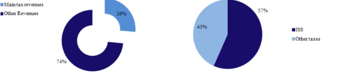
As shown in Ągure
1
, the tax revenue corresponds to around 30% of the countiesŠ
revenue in the São Paulo state (average), and considering this, the ISS corresponds to
50% of the collection of taxes, thus providing 15% of the total revenue of these localities,
on average, according to the database Brazil Finances (Finbra) for the year of 2012. This
data prove the relevance of this tax for the county collection, and therefore it is important
to seek results that can aid in the debate on the tax policy of the counties.
Figure 1 Ű A-Average participation of tax revenues on total revenue B-Average
participation of ISS on tax revenues
Notes: Average for all municipalities of the state of São Paulo. Source: Finbra 2012.
As already mentioned, the tax competition literature (WILSON, 1999) indicate
2
Barcellos (2004) studies the specific cases of Barueri and Santana de Parnaíba, studying the effects of
that the equilibrium tax rates in a context of competition can be excessively low, afecting
the tax collection, which therefore would translate into a low level of provision of public
goods. Since the ISS is a tax rate that directly afects the revenues of service companies
then, it is important in the locational decision of businesses, which can lead the local
governments to compete through taxes to attract Ąrms. Therefore, the analysis of the ISS
rates is relevant in order to present how the local taxes are deĄned in practice, checking if
the evidence conĄrms some of the predictions from the tax competition literature.
This work intends to investigate the main variables that inĆuence the choice of
the rates in the municipal level. It also aims to investigate the strategic interaction of
the counties in the process of the tax rateŠs deĄnition, trying to identify if there is any
relationship between the rates of a determined locality and its neighbors. For these purposes,
the data from the São Paulo state will be used. It is worth realizing that since there
is no uniĄed base of rates on municipal taxes, a compilation of the municipal data was
performed for this work, thereby being an additional contribution for future studies. Given
the data availability, the econometric analysis will be in cross-section.
In order to fulĄll these goals, an econometric model of the main determinants
of the ISS rates will be estimated. Among the explanatory variables, besides the local
characteristic variables, the average ISS rate of neighboring municipalities will be included
in order to assess the interaction between localities in the tax rate setting. Due to the
inclusion of variables of neighboring cities, the econometric models will make use of spatial
econometrics methods. The base model to be used is the Spatial Durbin Model, which
adheres better to the data, as will be shown in the development of this work. The empirical
strategy will be to explore the diferent service sectors studied, analysing how the estimates
vary between the groups. A Tobit model will also be estimated, in order to take into
account the possibility of limited reaction functions, as presented in Porto and Revelli
(2013).
Moreover, the issue of selection of the spatial weights matrices is also addressed
comparison, in order to select the matrices that best Ąt the data, following the work of
Stakhovych and Bijmolt (2009).
The rest of this dissertation is divided as follows: section 2 and its subsections
present a brief revision of tax competition and the theoretical bases of the study; the
data is presented in section 3; section 4 presents the methodology to be used; in section 5
the results are presented and analyzed; and the Ąnal summary and conclusion is made in
2 Tax competition and local government interaction
2.1
Tax competition theory
Wilson (1999) presents a broad review of the tax competition literature. The tax
competition theory extends the Tiebout (1956) model to include the externalities that
result from local governments actions, such as the impact on the other regionsŠ tax bases.
In the Tiebout model, each region has a government controlled by a landowner,
and they seek to maximize the value of the local lands. It can be extended to Ąrms, by
stating that there is an inĄnite supply of Ąrms in any region. This model relies in a special
design where governments can tax the local citizens eiciently. With that arrangement,
the model leads to eicient tax competition, with localities setting their tax rates exactly
at the level of provision of their public goods.
The tax competition theory then extends the model to include the externalities
generated by government actions. When a local government raises (reduces) its tax, it
generates an externality, increasing (reducing) the capital level in the other regions. This
beneĄt is not taken into account by the local government, meaning it sets tax rates
and levels of public goods at ineiciently low levels. This is an important result of the
tax competition theory, being a signiĄcant reason for the centralized taxation and grant
systems adopted in several countries.
Some special cases have also been studied in the literature, such as the case where
there are large regions competing
1. These regions afect the return on capital (r), therefore,
the total cost of capital (r+t
2) is less sensitive to tax rate changes in the large region.
This means the outĆow (inĆow) of businesses due to an increase (decrease) in the tax
rate is less severe in the larger regions. This allows the large regions to have higher taxes
compared to small regions.
1
Bucovetsky (1991) and Wilson (1991)
2.2
Approaches to identify local interaction
The international literature on local government interaction is quite signiĄcant,
with studies for several countries and diferent institutional arrangements. These studies
vary in the empirical methodology and identiĄcation strategy implemented. There are
some studies that use: i) spatial lag models or IV, combined with electoral information to
identify the interaction, mainly in yardstick competition models
3; ii) spatial lag models
or IV combined with exogenous policy shocks or particular institutional arrangements
4.
Below are some examples of these approaches.
Edmark et al (2008) uses an instrumental variables approach combined with auxiliar
equations to identify the spatial correlation in the income tax rates set by municipalities
and the source of the correlation. Following Kelejian and Prucha (1998), the authors
estimate a 2SLS model using neighborsŠ unemployment rate and share of welfare recipients
as instruments. The results show a strong correlation between their own tax rates and the
tax rates of neighboring jurisdictions. Additionally, the authors test for tax competition
and for yardstick competition. First, they test if a legislation change, which afected the
incentive to the tax competition, had signiĄcant impact in the interaction among localities.
Secondly, they make use of electoral information to test if the elections had any impact in
the tax interaction. The results indicate that the yardstick competition is not relevant in
that case, and that the tax competition has a small impact.
Elhorst and Fréret (2009) estimate a spatial Durbin Model
5, allowing the coeicient
of interaction to be diferent in two regimes, deĄned as departments governed by a large
political majority and departments governed by small political majorities in the council.
The results show that the spending in French departments is inĆuenced by yardstick
competition. The estimation shows that localities which have a small political majority
3
Besley and Case (1995), Revelli (2002), Bordignon, Cerniglia and Revelli (2003), Feld, Josselin and
Rocaboy (2003), Allers and Elhorst (2005), Edmark et al (2008), Elhorst and Fréret (2009), Videira
and Mattos (2011) and Menezes (2012).
4
Brett and Pinkse (2000), Brueckner and Saavedra (2001), Buettner (2001), Reulier and Rocaboy
(2009)
5
A model that includes WY and WX (the spatial lag of the dependent and independent variables),
present stronger interaction with neighboring spending than the localities with large
majorities, which is in line with yardstick competition theory.
Brueckner and Saavedra (2001) present a test of the presence of tax competition in
the cities in the Boston metropolitan area. After deriving a theoretical model, the authors
estimate a reaction function for the localities, using spatial lag models with diferent
weight matrix speciĄcations. First, the authors estimate the model and Ąnd a high and
signiĄcant interaction among the localities, and then they estimate the models for the
years of 1980 and 1990, taking advantage of a legislation change that started in 1981 in
the state of Massachusetts, to test if the institutional change afected the interaction. By
comparing the results for these two years, it was possible to identify a small reduction in
the interaction among localities when setting the average tax rate.
Although the international literature is already quite extensive, in Brazil there are
few studies about the theme. Moreover, the studies for Brazil explore the areas of tax
revenue and tax expenditure, with a lack of analysis on tax rates at the local level. Among
the studies, Videira and Mattos (2011) and Menezes (2012) are highlighted, which analyze
the interaction among the counties through local expenses. The authors Ąnd results that
demonstrate a meaningful inĆuence of the policies of the neighbors in the expenses of
the local counties. The Ąrst study pointed out the expenses in investments, health and
education, analyzing the behavior in electoral and non-electoral years, in order to identify
the preponderant efects. The second one makes use of an institutional change in the
visibility of education performance to assess the efects on the interaction among localities.
The econometric analyses using spatial econometric panel models showed that there is a
positive relation between local expenditures and the expenditure of neighbor municipalities.
The results indicate that this correlation is likely caused by yardstick competition because
it is stronger and more signiĄcant in election years and the institutional change also caused
a positive efect in the interaction observed.
In this work, the empirical approach will be to estimate a spatial durbin model,
presentation of the data, the tax rates of the ISS can vary from sector to sector, which can
translate into diferent levels of interaction between local governments when setting tax
rates for diferent sectors. This means that sectors which are more relevant to the local
government and/or highly sensitive to tax competition should present a higher and more
signiĄcant coeicient of interaction. Comparing the diferent coeicients of interaction
estimated for the sectors can then contribute in the identiĄcation.
2.3
Theoretical model
As seen in the revision of the tax competition literature, diferent model
arran-gements can be used, but in general the main results hold in every model design. In
the theoretical formulation of the work, a similar structure will be used to the one used
in Hindriks et al (2008) and Buettner (2003). It deĄnes the equilibrium condition, the
well-being function and the production function in a way that can derive the equations of
capital allocation and the tax rate reaction function.
The subject of this study is the tax on services that afect directly the companies.
Then, the theoretical model will be based in a mobile capital factor, representing the
services companies. Well, in equilibrium this condition must hold:
��
(
�
i, �
i)
��
i⊗
�
i=
�
(2.1)
In which,
�
(
.
) is the function of production in which the conditions of Inada
6are
valid,
�
is the capital,
�
represents other attraction factors, and
�
is the interest rate
7,
meaning that the return on capital net of the tax rate
�
must be equal in all the localities,
matching the interest rate. Consider a world with two localities (i, j) and with the total
ofer of capital (
�
) Ąxed Ű normalized for 1.
6
Inada conditions:
��(�i,�i)��i
>
0,
�2�(�i,�i) ��2
i
<
0,
f
(0) = 0, lim
�i→+∞��(�i,�i)
��i
= 0, lim
�i→0��(�i,�i)
��i
=
+
∞
7
As stated in the brief revision of the tax competition literature, when there is a large locality in the
economy, the after-tax return on capital (
r
) is influenced by the tax rate set by the large locality .
The localities maximize a well-being function (
�
i) in the following way, as
�
as a
variable of choice:
�
i(
�
) =
�
i(
�
i, �
i)
⊗
�
i(
�
i)
�
i+
�
i�
i(2.2)
�
iis the production function and
�
iis the derivative of the production function
in relation to
�
. The well-being function shows that the interest is to maximize the local
production of the private consumption goods and of the public goods, net of the payment
of the capital factor, which is taken as a non-resident property.
The production function is stated in the following way:
�
i(
�
i, �
i) = (
Ò
+
�
i)
�
i⊗
Ó�
2 i2
(2.3)
This shows that
Ò
is a parameter and
Ó
⊙
1 is the rate of decline of the marginal
product of capital with the increase of capital invested in the place. With this formulation,
using the equilibrium condition presented in equation (2.1), it is possible to derive the
function that represents the capital level:
�
i=
1
2
+
(
�
i⊗
�
j)
⊗
(
�
i⊗
�
j)
2
Ó
(2.4)
This model makes clear the relation among the local attraction factors (
�
), as well
as the relation between the increase in the capital and the tax rate diferential. Finally,
the localities anticipate the allocation of capital and solve their maximization problem,
obtaining the following reaction functions
8:
�
i(
�
j) =
Ó
3
+
(
�
i⊗
�
j)
3
+
�
j3
(2.5)
The reaction function shows the relation with the tax rates of the neighbor localities.
The idea is that the parameter of interaction is as synthesis of the relation between the
local rates and the neighborhood.
To the general case, with more than two localities, considering that the factors that
8
For a more complete reaction function, Brueckner and Saavedra (2001) include preferences over public
attract and repulse companies may be approximated by speciĄc characteristics of each
locality,
�
ik(
�
is the number of exogenous variables), and their neighbors, the reaction
function would be:
�
i=
K︁
k=1
Ñ
k�
ik+
n︁
j=1 K
︁
k=1
å
i,jk�
jk+
n︁
j=1
Ú
i,j�
j(2.6)
This theoretical model may be understood as a dynamic model in which the process
of the deĄnition of rates by a county, and its reaction regarding its neighbors, happens
along the time, in a way that what is to be observed is an equilibrium result. LeSage and
Pace (2009), chapter 2, show a model where
�
(the rate in a locality) in the instant
á
is
inĆuenced by the rates of neighbors deĄned in
á
⊗
1:
�
i,τ=
n︁
j=1
��
i,j�
j,τ−1+
K︁
k=1
Ñ
k�
ik,τ+
n︁
j=1 K
︁
k=1
�
k�
i,j�
jk+
�
i,τ(2.7)
in which
�
i,jrepresents the relation of neighboring among the unities
�
e
�
, and
�
are
explanatory variables. DeĄning this relation of neighborhood to all the localities, through
a spatial weights matrix, W, in which
i)
�
i,j= 0 for
�
=
�
ii) 0
⊘
�
i,j⊘
1, for
�
̸
=
�
iii)
︁
nj=1
�
i,j= 1
Considering
�
(
�
)
t) = 0, this model has as limit expected value of
lim
τ→∞
�
(
�
τ) = (
�
n⊗
��
)
−1(
�Ñ
+
� ��
)
(2.8)
where X is a matrix of exogenous explanatory variables. This limit corresponds to the
expected value of an econometric model of the type SDM (Spatial Durbin Model), as
follows:
�
=
�� �
+
�Ñ
+
� ��
+
�
(2.9)
3 Data
3.1
Data source
To fulĄll the goals demonstrated, the ISS rates of the municipalities of São Paulo
state will be used, which demand a speciĄc research project performed by this work, being
an additional contribution for further studies. In general, this data is presented in the
Municipal Tributary Code and in the complementary legislation, not being compiled in a
uniĄed base
1. As seen during the collection, besides the diiculties in the compilation of
rates, which complicates the coverage of a longer period, a low variation of the tax rates
along the time has also been noticed. Thanks to these reasons, the rates collected are those
currently valid in the counties
2, in a way that the analysis will be made in cross-section.
In our survey, it was possible to collect the rates of around 538 counties of São
Paulo state
3. This number corresponds to 83% of the 645 counties of the state. These
collected localities represent more than 95% of the total ISS collection of the São Paulo
counties, thus being responsible for the biggest part of the service sector production in the
state.
The Ąnal sample used is composed of 511 counties, covering a great part of the
state. Twenty-seven cities were excluded due to the lack of Ąscal variables and (or) rates
for some groups of speciĄc services. The 134 absent cities (27 excluded + 107 not collected)
are predominantly small towns, at around 6,000 inhabitants, with a low collection of ISS,
as seen in the appendix A. These cities are also spatially well-distributed, as seen in the
map in appendix A, and in such way that there is no region in the state speciĄcally absent
in the base, making our sample especially representative of the state.
Each municipality deĄnes the ISS tax rates for 40 groups of services, besides the
subgroups in speciĄc cases. Thanks to the great variability of rates among the groups, it is
1
The Roads Department of the state of São Paulo (DER-SP) has a database of ISS rates for about 400
municipalities, since they collect road tolls for these localities.
2
The tax rates were collected in the end of 2014.
intended to estimate the models for each group separately, therefore avoiding problems
caused by an aggregation of diferent services. Also due to the great number of service
groups, the work will be done with only part of the groups. The choice of the groups to be
studied took into consideration the premise of tax competition. Many groups are local
services
4, very diluted and which would not be relevant to evaluate competition among
localities. The rates for these groups also present little variation among the localities, as
can be seen in the table of appendix B.
3.2
Presentation of the ISS data
Regarding the ISS rates, the legislation determined that the municipal
administra-tion may deĄne the rates of each group and subgroup, respecting the minimum (2,0%)
and maximum (5,0%) limits for the rate. The tax applies to the gross revenue of the
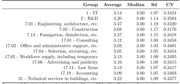
produced service. Table
1
and Ągure
2
present some descriptive statistics of the groups
and subgroups of service that will be studied
5:
Table 1 Ű Descriptive statistics of the selected groups - tax rates
Group
Average
Median
Sd
CV
1 - IT
3.14
3.00
1.07
0.3424
2 - R&D
3.20
3.00
1.14
0.3564
7.01 - Engineering, architecture, etc.
3.47
3.00
1.19
0.3420
7.02 - Construction
3.68
3.00
1.17
0.3176
7.13 - Fumigation, disinfection, etc.
3.37
3.00
1.15
0.3418
17.01 - Consulting
3.12
3.00
1.08
0.3458
17.02 - Office and administrative support, etc.
3.03
3.00
1.03
0.3401
17.04 - Selection, recruiting, etc.
3.05
3.00
1.05
0.3454
17.05 - Workforce supply, including temporary
3.13
3.00
1.09
0.3495
17.06 - Advertising and publicity
3.16
3.00
1.08
0.3415
17.14 - Law firms
3.13
3.00
1.07
0.3417
17.19 - Accounting
3.09
3.00
1.05
0.3403
31 - Technical services in buildings, etc.
3.22
3.00
1.09
0.3377
Source: Municipal tax legislation.Note: CV=Coeicient of variation.
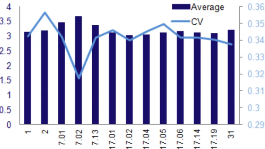
It is possible to see in Ągure
2
that the average tax rates are all above 3%, with
the subgroups of civil construction (group 7) presenting the highest averages. As for the
4
Services of health, education, transportation, Social assistance, personal cares, hotel business, leisure,
veterinary medicine, among others.
5
They correspond to the following codes of the Services Table from the ISS legislation: 1, 2, 7.01, 7.02,
Figure 2 Ű Average and Coeicient of Variation for ISS rates by group of service
Source: Municipal legislation. Own elaboration.
variation, it is possible to see that the biggest variation happens in the Research and
Development group (group 2), followed by the service of workforce supplier (subgroup
17.05). The highlight is to the subgroup 7.02 Ű civil engineering works Ű which present a
high average and a low variation among the localities.
The maps in Ągure
3
represent the ISS rates for some selected service groups. It is
possible to notice that the spatial distribution varies from group to group. Some present a
higher average, shown by the stronger colors. Others have the lighter maps, which presents
the lowest rates on average, as seen in groups 1 and 2. It is also possible to see in the
maps a great variety of rates. There is a predominance of higher rates in the counties of
the western region, closer to the border of the state. In the lighter maps, it is possible to
see that the big cities that are Micro Region Centers present higher rates, such as in São
Paulo, Campinas, Sorocaba, and Marília (these cities are highlighted in the red circles of
group 1), among others. It is possible to see several points of higher rates amongst the
cities with lower rates. The maps are illustrations to contextualize the spatial analysis.
In Ągure
4
, it is possible to notice that the average of the ISS rates, for all the groups
and subgroups, is higher in the localities that do not take part in the urban agglomeration
areas, as shown by the diference between the general average and the average in the areas
Figure 3 Ű Maps of the ISS rate distribution over space
cities that are Micro Region Centers
6(MR) have an average of higher rates, around 7%
higher, than the others in their MR. This observation is aligned with the agglomeration
theory, as seen in Baldwin and Krugman (2004), with the cities that are MR centers being
able to keep higher rates due to the gains from the agglomeration, partially compensating
the higher tax burden for the companies.
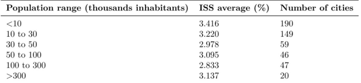
The distribution of the taxes between the diferent population ranges is also
interesting, as showed in table
2
. It is possible to notice that smaller cities have higher
ISS rates on average. The observed average is inversely proportional to the population,
exception made to the group of cities from 50 thousand to 100 thousand inhabitants and
Figure 4 Ű Average ISS rate for diferent groups of cities
Source: Municipal legislation. Own elaboration.
to the larger cities (larger than 300 thousand inhabitants). These observations give some
insight of how municipalities set the ISS tax rates. It seems that small cities set higher
taxes, while as cities get larger they start setting lower tax rates, exception made to the
very large cities, which in line with the tax competition literature
7set higher taxes due to
the agglomeration gains.
Table 2 Ű Average ISS rate according to population size
Population range (thousands inhabitants)
ISS average (%)
Number of cities
<10
3.416
190
10 to 30
3.220
149
30 to 50
2.978
59
50 to 100
3.095
46
100 to 300
2.833
47
>300
3.137
20
Own Elaboration
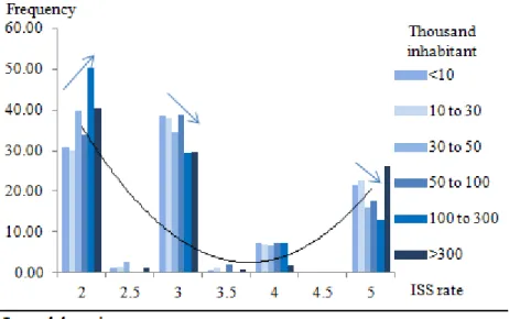
Complementing these evidence, Ągure
5
presents the distribution of the ISS rates
according to the population size of the localities. It shows that the percentage of
muni-cipalities setting rates at the 2p.p. level increases with the average size of the localities,
while the percentage of higher taxes decrease with the population size (the arrows make
clear this observation). These Ąndings reinforce the idea that as cities get larger they start
setting lower tax rates, likely engaging in more tax competition.
Finally, since the subject is the tax rates deĄnition and the likely use of the taxes
Figure 5 Ű Distribution of rates for diferent population sizes
Source: Municipal legislation. Own elaboration.
to attract companies, it is important to analyse the data on employment in these sectors
in the localities of the sample. In the table
3
, there is information about the average
level of employment, the variation and the concentration of the employment in each
sector in the sample analysed. It is worth noting that the Construction and Consulting
are the less spatially concentrated groups, meaning that the number of localities with a
positive level of employment in these sectors is higher than the others. The table also
shows that Construction, Workforce supply and IT are the groups with the highest level of
employment, on average. These data should help in the analysis of the empirical results.
Table 3 Ű Descriptive statistics - employment by sector in the sample of 511
municipalities
Group Average Median Sd Max Min Concentration index*
1 - IT 286.02 0.00 3566.60 77320 0.00 57% 2 - R&D 16.75 0.00 185.13 3062 0.00 88% 7.01 - Engineering, architecture, etc. 144.33 1.00 1626.88 36203 0.00 48% 7.02 - Construction 1149.99 44.00 11469.58 256118 0.00 15% 7.13 - Fumigation, disinfection, disinsectization, etc. 18.31 0.00 147.23 2345 0.00 55% 17.01 - Consulting 165.93 2.00 1845.14 40703 0.00 39% 17.02 - Office support and administrative infrastructure, etc. 158.42 2.00 1976.18 43950 0.00 42% 17.04 - Selection, recruiting, etc. 73.80 0.00 780.40 16748 0.00 82% 17.05 - Personnel supply, including temporary 373.56 0.00 3827.98 83171 0.00 75% 17.06 - Advertising and publicity 10.95 0.00 176.69 3970 0.00 86% 17.14 - Law firms 49.56 1.00 758.16 17023 0.00 49% 17.19 - Accounting 12.13 0.00 97.35 2011 0.00 76% 31 - Technical services in buildings, electronics, etc. 27.27 0.00 242.00 5302 0.00 60%
3.3
Presentation of the explanatory variables
Before presenting the explanatory variables it is important to discuss about the
demographic variables. These variables are an important subject, since the deĄnition of
the tax rates likely depend on them, specially on the population size of the localities. Also,
the tax decision of local governments afect the incentives for economic agents, and one of
the possible consequences of these tax decisions is the migration of the tax base/payers to
other localities, which would then inĆuence the population size, being a possible source
of endogeneity in the model. Due to that possible problem, before adding demographic
variables in the model, it is important to evaluate some data about migration and the ISS
rates.
The possible problem of endogeneity would come up if the diference in ISS rates
across localities led to migration. According to the tax competition literature (Wilson,
1999) this would happen if the diference in ISS rates increased/decreased the number of
jobs in a locality given its lower/higher tax rates. Also, this migration efect would happen
if the change in employment level was signiĄcant enough compared to the population
size. Then, Ąrst of all, it is important to analyse the level of employment of the services
sectors being studied in this work. The thirteen sectors represent only 9.4% of the formal
employment in the localities on average
8. More importantly, the data also shows that
the population growth in recent years is not correlated with the growth in employment
in the service sectors being studied
9. This evidence show that the relation between the
employment growth and the efects on migration do not seem so signiĄcant for the ISS
case being studied, or at least, these efects are not so clear in the data.
Given that, the data shows that the possible efects of the ISS rates on migration
are likely limited. However, to further minimize the possible endogeneity of these variables,
the population variable will not be included directly in the model. A variable will be
8
Corresponding to about 17.5% of the formal employment in Services, since formal Services employment
is 53.9% of the total – source Seade, 2014.
9
Population growth between 2014 and 2010 compared to the employment growth (RAIS, source:
included to represent the relative size of the municipalities on its Micro Region, as a
way of presenting the structural dimension of the locality on its economic region. That
is, that variable can show if the municipality is larger/smaller than the average of the
municipalities in its economic region, which could indicate the economic attractiveness of
the locality, afecting its tax decision.
For the other control variables, we followed the literature on tax interaction (Edmark
et al (2008), Allers and Elhorst (2005), Bordignon, Cerniglia and Revelli (2003), etc.).
The idea was to select the variables that could inĆuence the tax deĄnition in diferent
dimensions, the social, demographic, economic characteristics, etc. Several variables were
tested in these diferent groups. The groups of explanatory and control variables used are
the following:
Economic structure variables: familiar income per capita; Economically Active
Population over the total population; dummy if the municipality is a center of Micro
Region (1 if it is a center of MR).
Demographic variables: dummy of population between 100 and 200 thousand
inhabitants
10(1 if the population is in this range); relative size: local population over the
average population in the micro region Ű the square of this variable is also included, to take
into account the non-linearity seen in the efects from populational variables; percentage of
elderly in the population Ű proxy to commitment with the provision of public services; %
pop with 25 years or more that have a high school, undergraduate or graduate degree, to
characterize the formal education of the local population, which can inĆuence the action
of legislators.
Fiscal variables: Grants per capita Ű quota from the Municipal Participation Fund
(FPM).
Additional variables: dummy if the county uses the donation of lots as a means of
attraction of projects (1 if it uses it)
10
Dummies were tested to different population divisions, but they didn’t explain the variation, and
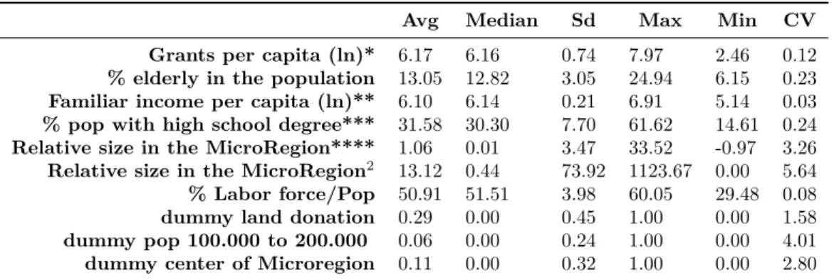
Table 4 Ű Descriptive statistics of the variables
Avg
Median
Sd
Max
Min
CV
Grants per capita (ln)*
6.17
6.16
0.74
7.97
2.46
0.12
% elderly in the population
13.05
12.82
3.05
24.94
6.15
0.23
Familiar income per capita (ln)**
6.10
6.14
0.21
6.91
5.14
0.03
% pop with high school degree***
31.58
30.30
7.70
61.62
14.61
0.24
Relative size in the MicroRegion****
1.06
0.01
3.47
33.52
-0.97
3.26
Relative size in the MicroRegion
213.12
0.44
73.92
1123.67
0.00
5.64
% Labor force/Pop
50.91
51.51
3.98
60.05
29.48
0.08
dummy land donation
0.29
0.00
0.45
1.00
0.00
1.58
dummy pop 100.000 to 200.000
0.06
0.00
0.24
1.00
0.00
4.01
dummy center of Microregion
0.11
0.00
0.32
1.00
0.00
2.80
Notes: *FPM; **Census, 2nd quartile; ***% of the population with more
than 25 years with high school degree or upper level degree;****This variable
is calculated as: (Local population-Average population in the MR)/Average
population in the MR; Source: Census 2010, Finbra, ProĄle of brazilian
municipalities, 2012 - IBGE
In most part the information is available from the Brazilian Institute of Geography
and Statistics (IBGE). The Ąscal variables come from the Brazil Finances database
(FINBRA), available on the site of the National Treasure. For the São Paulo state, this
information may also be obtained on the Seade portal, the Foundation State System of
Data Analysis. All the data is taken as reference to the year of 2010
11, to align with the
last available census. More information can be found in the table of descriptive statistics.
3.4
Concentration of the ISS rate
As previously mentioned, the ISS rates are discretionary but limited in a range
between 2% and 5%. It is likely, then, that for some cities the choice of the optimal tax
rates should be a corner solution.
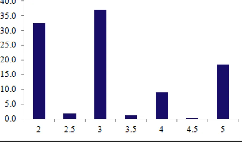
The histograms and table
5
show that the tax rates are concentrated on three
values, 2, 3 and 5p.p., and around 90% of localities set their tax rates within these three
levels. On average, 38% of the governments set ISS rates at the level of 3p.p. The level of
2p.p. follows, with an average of 30%, and the value of 5p.p. shows an average of 23%.
These statistics corroborate the view that the tax limits imposed by federal law may lead
to corner solutions in the tax setting. In that case, a Tobit model should be implemented,
Table 5 Ű Frequencies of the ISS tax rates - %
2
2.5
3
3.5
4
4.5
5
1 - IT
32.49
1.76
36.99
1.17
8.81
0.20
18.59
2 - R&D
32.88
2.15
33.86
0.98
6.65
0.20
23.29
7.01 - Engineering, architecture
25.24
0.78
33.46
0.20
7.83
0.20
32.29
7.02 - Construction
18.40
1.37
31.31
0.78
9.59
0.20
38.36
7.13 - Fumigation, disinfection, etc.
25.83
0.98
37.96
0.59
6.07
0.20
28.38
17.01 - Consulting
33.27
0.78
38.55
1.57
6.26
0.20
19.37
17.02 - Office and admin. support
34.83
1.37
40.51
1.37
5.48
0.20
16.24
17.04 - Selection, recruiting, etc.
35.42
0.78
39.73
1.57
4.89
0.20
17.42
17.05 - Workforce supply
33.46
0.98
38.55
1.57
4.89
0.20
20.35
17.06 - Advertising and publicity
31.31
1.17
38.36
1.57
7.63
0.20
19.77
17.14 - Law firms
31.51
1.17
41.10
1.37
5.09
0.20
19.57
17.19 - Accounting
32.88
1.37
40.51
1.37
5.87
0.20
17.81
31 - Technical services in buildings
28.18
1.17
41.29
1.57
5.87
0.20
21.72
Level of signiĄcance: ***1%;**5%;*10%
Figure 6 Ű Frequency of the ISS rates - group 1 - IT
Source: Municipal legislation. Own elaboration.
as to better estimate the reaction function of the municipalities.
Figure 7 Ű Frequency of the ISS rates - group 17.01 - Consulting
4 Methodology
4.1
Matrix selection
The spatial econometric approach takes use of weight matrices (W) in order to solve
the problem of excessive parameters because if it is intended to directly include the variables
of neighbors in the equation, it would not possess suicient degrees of freedom. Therefore,
the use of weight matrices is a way of making the model more parsimonious. The matrix W
may present several forms, always trying to represent the relation among the neighbors. In
the literature, the most common matrix is the binary contiguity (WBC), which considers
neighbors as the localities that share borders. From that notion of neighborhood, each
neighbor gets the same weight (unitary) and as the neighbors of each locality are deĄned,
the matrix W of dimension n x n is created. Afterwards, the matrix is normalized in the
line, in order to make clearer the interpretation of the results..
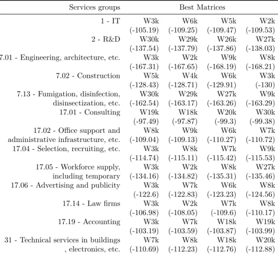
One criticism about spatial econometrics analysis is the choice of the spatial weights
matrices (LESAGE and PACE, 2014). In most parts of the literature, the selection of the
matrices is ad hoc, based only in theory and not in statistical tests. To choose the most
appropriate matrix, it is possible to compare the log-likelihood of the models estimated
by Maximum Likelihood. Stakhovych and Bijmolt (2009) pursue a simulation study,
showing that a selection procedure for the weights matrix based on the log-likelihood, or
information criteria, usually indicates the correct speciĄcation. Besides that, the authors
also show that spatial models which use a binary contiguity weight matrix (WBC) perform
better on average than do those that use other weight matrix speciĄcations, due to their
higher probabilities of detecting the true model and the lower mean standard error of the
estimated parameters. Therefore, in this study, the models will be estimated with the
weight matrices that best Ąt the data, according to the log-likelihood, and with the binary
contiguity matrix, which is the most common one in the literature and presents a good
4.2
Base model - SDM
The practical approach will take use of the spatial econometric techniques,
iden-tifying the parameters of the main variables that determine the tax rate setting, including
the tax rate from neighbor municipalities. Anselin (1988) is the main reference in the
spatial econometric literature. Many developments have occurred after this work and the
majority of the most recent techniques are shown in the book by LeSage and Pace (2009),
on which the models used here are based. The speciĄcation strategy follows the classical
approach, starting out of a simpler model to a more complete one, taking use of spatial
correlation tests and speciĄcation tests for the right model. As presented in Florax and
Rey (2003), the classical approach is more eicient than the approach of HendryŠs type,
which, unlike the classical one, starts from the more complex model to the simple one.
Following the estimation presented in Allers and Elhorst (2005) and Bordignon
et al (2003), the speciĄcation process of the spatial interaction must be initiated with
a regression of ordinary least squares (OLS), in order to apply the MoranŠs I test on
the residuals, identifying if there is spatial dependence on the observed data. After this
analysis, further tests are performed in order to specify the most appropriate model.
As showed in the presentation of the data, the model will be estimated in
cross-section for each group of service. As already shown in the theoretical cross-section, cross-cross-section
models must be observed as the representation of an equilibrium result, meaning the
estimated parameters that relate the variable of locality i to the locality j do not necessarily
represent an instantaneous relation. SpeciĄcally in the tax rates case, it is reasonable to
expect that the process of setting the tax rates does not happen automatically, with the
equilibrium of rates observed in a moment in time being a result of a longer interaction
process.
In summary, the steps for the estimation are:
I) OLS
with
�
ga vector (n x 1), containing the ISS rates of a determined group of services
(g) for each of the n counties, X a matrix (n x k), containing the control variables,
Ñ
a
parameter vector (k x 1) and the error term
�
g≍
�
(0
, à
2).
II) Moran’s I and LM tests
The spatial correlation test, MoranŠs I, is performed using the residues of the OLS
estimation, followed by the LM speciĄcation tests, robust and non-robust. Following the
test results, the tests of the models SDM and SDEM were performed, leading to the SDM
model as the most appropriate:
III) Estimation of the Spatial Durbin Model
As it will be shown by the test results, the Spatial Durbin Model was the most
appropriate to the identiĄcation of the countiesŠ interaction. This model is deĄned in the
following way, according to LeSage and Pace (2009):
�
g=
�� �
g+
ÐØ
n+
�Ñ
+
� ��
+
�
(4.2)
with W being a spatial weights matrix (
�
x
�
),
Ø
na vector n x 1 of entrances 1. (
�, Ð, Ñ
and
�
) are parameters,
Ñ
and
�
are n x k,
�
and
Ð
are scalar.
This model shows that the rates of a locality depend on the pondered rates of their
neighbors
� �
, of their explanatory variables
�
, as well as the explanatory variables of the
neighbors,
� �
. On this speciĄcation, the parameter
�
deserves special interest, since it
presents the magnitude and the direction of the interaction among the counties to deĄne
the rates, on average. Also, the exogenous variables in
�
and
� �
can show signs of the
presence of tax competition among the municipalities.
Due to the endogeneity of the model, shown by the presence of the dependent
variable
�
appearing also as an explanatory, in
� �
, it is necessary to rewrite the model:
�
g= (
�
n⊗
��
)
−1