EXPERIMENTAL EVALUATION OF A CASCADE CONTROL TECHNIQUE
WITH FRICTION COMPENSATION FOR A FLEXIBLE JOINT ROBOT
A. R. G. Ramires
∗E.R. De Pieri
†R. Guenther
‡In Memoriam
J. F. Golin
‡∗University of Vale de Itajaí, Computation Engineering, Campus São José
Rodovia SC 407, Km 4 88122-000 São José-SC, Brazil
†Department of Automation and Systems, Federal University of Santa Catarina
88040-900 Florianópolis, SC, Brazil
‡Department of Mechanical Engineering, Federal University of Santa Catarina
88040-900 Florianópolis, SC, Brazil
ABSTRACT
This paper focuses on the experimental results of the posi-tion tracking control of a flexible joint robot manipulator. The applied control strategy is based on a well know cas-cade control methodology that divides the robot model into two subsystems: a link and a rotor subsystem. Thanks to this division a friction compensation based on the LuGre model is performed to the mechanical system. The main goal of the present work is to apply a systematic procedure to iden-tify the friction model parameters and to analyse the control strategy performance when implemented to a robot prototype specially built for practical tests.
KEYWORDS: Robot control, joint flexibility, friction
ob-server, friction compensation, cascade control.
RESUMO
Controle em Cascata com Compensação de Atrito para Robôs com Juntas Flexíveis: Teoria e Resultados
Experi-Artigo submetido em 20/12/2007 (Id.: 00841)
Revisado em 01/04/2008, 15/09/2008, 03/12/2008, 18/04/2009
Aceito sob recomendação da Editora Associada Profa. Anna Helena Reali Costa
mentais
Neste trabalho são apresentados resultados experimentais de seguimento de trajetória de posição de um robô manipulador com flexibilidade nas juntas. A estratégia de controle é base-ada na metodologia do controle em cascata, dividindo o mo-delo do robô em dois subsistemas: o subsistema dos elos e o subsistema do rotor. Essa abordagem facilita a compensação do problema de atrito do subsistema mecânico ou dos elos. Usou-se para a compensação de atrito o modelo de LuGre. O principal objetivo da abordagem apresentada é fornecer um procedimento sistemático para identificação dos parâmetros do modelo de atrito e a análise de desempenho da estraté-gia proposta quando aplicada a um protótipo especialmente construído para testes experimentais.
PALAVRAS-CHAVE: Controle de Robôs, Robôs Flexíveis,
Observador de Atrito, Controle em Cascata
1
INTRODUCTION
the elastic coupling introduces an additional degree of free-dom at each joint. In particular, a robot with flexible trans-missions has the double of degrees of freedom with respect to its rigid equivalent. Thus, this robot is apartially actuated system, since it has2nvariables to be controlled through only
ncontrol torques. Therefore, the usual methods for tracking
control, such as the inverse dynamics formulation and the control based on Lyapunov, cannot be directly applied to that system (Readman, 1994).
Different control strategies for elastic joint robots have been developed in the literature. Among those strategies, one may cite PD control (Tomei, 1991; Dupont, 1994), dy-namic feedback linearization methods, singular perturbation theory, robust and adaptive schemes (Nicosia and Tomei, 1988; Tomei, 2000), integrator backstepping based method-ologies (Nicosia and Tomei, 1992) and cascade methodolo-gies (Guenther and Hsu, 1993).
There are some important differences between those tech-niques. A basic comparative study can be found in (Brogliato et al., 1995). PD controllers, which work well for industrial robots, add some damping for the joint elasticity but their performance and robustness are very limited. The controller bandwidth has to be reduced until robustness against highly nonlinear dynamics is reached. Stability proofs for such con-trollers are more complicated than for the concon-trollers using extensive model information. The singular perturbation is a simple two stage method, referred as corrective control, but it only works well in the case of weak flexibility. Adap-tive versions of that control technique have been developed with good results (Ghorbel and Spong, 2000). An exten-sion to consider the problem of position and force control of uncertain constrained flexible joint robots was presented in (Huang et al., 2006). The dynamic feedback linearization methods are quite simple to be used but in the most general cases the dynamics of flexible joint robots are not feedback linearizable. Also, the main disadvantage of feedback lin-earization is the necessity of the exact knowledge of the robot parameters and the need of joint acceleration and jerk mea-surements.To overcome these difficulties, adaptive and pas-sivity based control techniques have been proposed (Fantoni and Lozano, 2000; Albu-Schäffer and Hirzinger, 2001). The backstepping schemes use the cascade decomposition prop-erty of the robot model (Kokotovic and Sussmann, 1989). The backstepping is a systematic procedure to control non-linear systems but the designer should pay attention to over-parametrization and time consuming computations. These latter are more involved than compared to the traditional cascade control procedure, for example. Also, in some al-gorithms, the measurement of joint accelerations is neces-sary. Using the cascade control methodology, a robust track-ing of a reference model, avoidtrack-ing overparametrization, was achieved (Wang and Khorrami, 2000). The cascade control
schemes also use the system decompositions in small subsys-tems. The overall system is partitioned in such a way that the states of the first subsystem are the control variables to the following subsystem. In this technique, the model uncertain-ties can be taken into account by using an adaptive control scheme. With this methodology, the problem of measuring joint accelerations can be circumvented.
In robots with joint flexibilities, some important phenom-ena like actuator dynamics and friction are not accurately included in the design of control algorithms (Lozano et al., 1997; Ramirez et al., 2003). In fact, friction occurs in all me-chanical systems,e.g. bearings, transmissions, hydraulic and pneumatic cylinders, valves, brakes and wheels (Canudas De Wit et al., 1995; Canudas De Wit and Lischinsky, 1997; Guenther et al., 2006; Lischinsky et al., 1999; Guenther and Perondi, 2004). In electrical driven robots the friction is al-ways present in transmission mechanisms, rotor and joints (Canudas De Wit et al., 1995). Friction can lead to steady state or trajectory tracking errors (Dupont, 1994; Guen-ther and Perondi, 2002; Ramirez et al., 2002) or can lead to cycle limites in flexible robots as shown in (Jeon and Tomizuka, 2005). Friction compensation is desired to cir-cumvent these problem and it is particularly difficult to be performed using a non-model based compensation (Lozano et al., 1997; Tomei, 2000) or even using a model-based com-pensation (Armstrong-Hélouvry, 1993; Canudas De Wit and Lischinsky, 1997) or using adaptive techniques (Xie, 2007).
Several models have been used to describe the friction phe-nomenon dynamics. In (Gomes and Santos da Rosa, 2003) a model is proposed to compensate friction effects. In a dif-ferent structure (Canudas De Wit et al., 1995; C. Canudas de Wit, 2007) develop a friction estimation scheme based in the LuGre model to build a model-based fiction compensation. In (Gandhi et al., 2002) an extension of the LuGre model is proposed to compensate friction in harmonic drives. Re-cently, a Generalized Maxwell-Slip model has been proposed by (Al-Bender et al., 2005) to describe the friction dynamics.
are not external forces. Experimental results illustrate the main properties of the proposed controller with the friction compensation model.
This paper is organized as follows. In Section 2, the model of the flexible joint robot manipulator with friction is recalled. The cascade control with friction compensation is proposed in Section 3. In Section 4, the stability of the proposed con-troller is demonstrated. Section 5 describes the off-line pro-cedure for the identification of friction parameters. In Sec-tion 6, the experiment is presented.
2
MODEL OF RIGID AND FLEXIBLE
ROBOTS WITH
N
LINKS
A mathematical model of a robot withnrigid links connected
bynrotational or translation rigid joints is given by (Canudas
De Wit et al., 1996)
M(q1)¨q1+C(q1,q˙1) ˙q1+G(q1) =τ (1)
where the vectorsq1,q˙1 andq¨1 represent, respectively, the
link position, velocity and acceleration, M(q1)is the
iner-tia matrix, C( ˙q1, q1)represents the centrifuges and
Corio-lis terms, G(q1)represents the gravitational torques and τ
is the control input. As pointed out in (Canudas De Wit et al., 1996), the elastic effects are small and can be ne-glected, the inertia matrix M(q1) is symmetric and
posi-tive definite and both M(q1) and M−1(q1) are uniformly
bounded for all q1 ∈ ℜn, and a convenient choice of
C( ˙q1, q1)leads to an skew-symmetric matrixM˙ −2C. This
system is consideredcompletely actuated in the sense that
one torque is provided for each degree of freedom.
In order to obtain the mathematical model of a flexible joint robot, the links are supposed to be rigid, the joint flexibil-ity is modeled as a torsional spring for rotational joints and as a linear spring for prismatic joints, and the inertia ma-trix takes into account the individual inertia of the links and rotors (Spong and Vidyasagar, 1989). Then, the dynamical model of a flexible joint robot can be written as
¯
M(q1)¨q+ ¯C( ˙q, q) ˙q+ ¯G(q1) + ¯Kq= ¯τ (2)
whereq1is associated to the position on the link,q2is
asso-ciated to the position on the rotor andqT =
qT 1 q2T
. The
elementsM¯(q1),C( ˙¯ q, q),G(q¯ 1),K¯ andτ¯are described in
(Canudas De Wit et al., 1996).
With the hypothesis introduced by (Tomei, 1991), (Canudas De Wit et al., 1996) and (Spong, 1987), it is possible to obtain a simplified model, given by
M(q1)¨q1+C(q1,q˙1) ˙q1+G(q1) =K(q2−q1)
Jq¨2+K(q2−q1) =τ
(3)
q1,q˙1 q2,q˙2
q2,q˙2
Rotor Subsystem
Link Subsystem
K(q2−q1)
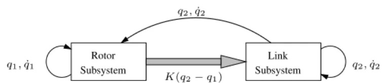
Figure 1: Cascade representation of flexible joint robots.
with J = diag(J1, J2, . . . , Jn), Jj being the inertia
asso-ciated to the rotor j, andK = diag(K1, K2, . . . , Kn),Kj
being the spring coefficient associated to jointj. Some robot
configurations can be adequately modelled by (3), like ma-nipulators with one rotational joint and one link or manipula-tors with two rotational joints and two links with perpendic-ular axes. In general, when the transmission reductions are important (for example when harmonic drivers are used) the simplified model (3) is valid.
The mathematical model (3) can be interpreted as two cou-pled subsystems: the first one represents the rigid robot model and the second one corresponds to the flexible joint dynamics. The coupling between the two models is given by the elastic torque represented by the termK(q2−q1). The
cascade interconnection of the two subsystem is shown in Fig. (1).
From the control point of view, the simplified model (3) de-scribes a non negligible elastic displacement between each link and its corresponding rotor. On the other hand, the whole system becomes partially actuated, since for2nequations describing the dynamical behavior of the system there are onlyntorque inputs. The main consequence of this behavior
is to limit the application of classical controllers (as P, PD and PID) normally used to control rigid manipulators. Fur-thermore, for an effective control of flexible joint robots it is necessary to use more elaborated control strategies (possibly with friction compensation) and to take into account some robustness requirements.
2.1
Friction Model
In this paper, the LuGre model (Canudas De Wit et al., 1995) is used to represent the friction. This model can describe complex friction behavior, such as stick-slip motion, pre-sliding displacement, Dahl and Stribeck effects and frictional lag.
The friction force is given by
F = Γ0z+ Γ1z˙+ Γ2q˙1 (4)
wherezis an internal state that describes the average elastic
deflection of the contact surfaces during the stiction phases,
Γ0 is a diagonal matrix of the stiffness coefficient of the
displace-ments, Γ1 is a diagonal matrix of the damping coefficients
associated withz˙andΓ2is a diagonal matrix that represents
the viscous friction.
The dynamics of the internal statezis expressed by
˙
z= ˙q1−Γ0Ψ( ˙q1)z (5)
with
Ψ( ˙q1) = diag
|q˙11|
g( ˙q11)
, . . . , |q˙1n| g( ˙q1n)
(6)
whereg( ˙q1i)fori= 1, . . . , nis a positive function that
de-scribes part of the steady state characteristics of the model for constant velocity motions. This function is given by
g( ˙q1i) =Fci+ (Fsi−Fci)e−
“q˙1i vsi
”2
(7)
whereFciis the Coulomb friction, Fsi is the static friction
andvsiis the Stribeck velocity and as stated in (Canudas De
Wit et al., 1995), each functiong( ˙q1i)is upper bounded, i.e.,
0< g( ˙q1i)≤ai, fori= 1, . . . , n.
The simplified model (3) is modified to take into account the friction. Then,
M(q1)¨q1+C(q1,q˙1) ˙q1+G(q1) +F =K(q2−q1)
Jq¨2+K(q2−q1) =τ
(8)
3
CASCADE CONTROL WITH FRICTION
COMPENSATION
In this section, the cascade control with friction compensa-tion is proposed for systems that may be represented by the model (8). Initially, the following errors are defined
˜
q1=q1−q1d
˜
q2=q2−q2d
˙
qr1= ˙q1d−Λ1q˜1
s1= ˙q1−q˙r1
s2= ˙˜q2+ Λ2q˜2
(9)
whereΛ1 andΛ2are diagonal positive definite matrices of
gains,q1dis the desired link position,q2dis the desired rotor
position andq˙r1is a reference for the link velocity.
The system (8) can be transformed into two cascade subsys-tems with inputsvandq2using a suitable change of
coordi-nates given by
τ=J v+K(q2−q1) (10)
q2d=K−1ud+q1 (11)
wherevis the control applied to the rotor subsystem andud
is the control for the link subsystem.
q1,q˙1
q2,q˙2
Kq˜2
Controller Rotor Link
Trajectory
Figure 2: Cascade model.
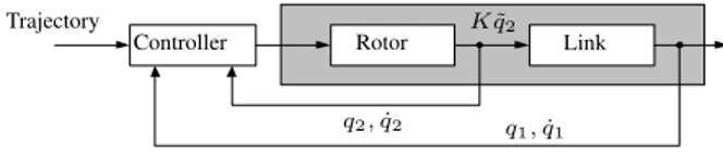
Substituting (10) and (11) in (8), the system is rewritten as
M(q1)¨q1+C(q1,q˙1) ˙q1+G(q1) +F =ud+Kq˜2
¨ q2=v
(12)
The robot system is then interpreted as an interconnected sys-tem like the one presented in Fig. 2.
The control project is performed through two steps: link con-trol and rotor concon-trol. In addition, a friction observer is de-signed.
3.1
Tracking Control of the Link
Subsys-tem
The controludis designed using the property of passivity in
robot manipulators(Canudas De Wit et al., 1996). Thus,ud
is given by
ud=M(q1)¨qr1+C(q1,q˙1) ˙qr1+G(q1)−KD1s1+ ˆF (13)
whereKD1is a diagonal positive definite matrix of gains and
ˆ
Fis the estimated friction torque.
The closed loop form of this subsystem is obtained substitut-ing (13) in the first equation of (12)
M(q1) ˙s1+ (C(q1,q˙1) +KD1)s1+F−Fˆ=Kq˜2 (14)
3.2
Tracking Control of the Rotor
Subsys-tem
The controlvis chosen as
v= ¨q2d−Λ2q˙˜2−J−1KD2s2 (15)
where KD2 is a diagonal positive definite matrix of gains.
Then, the control torqueτis given by
τ=J(¨q2d−Λ2q˙˜2)−KD2s2+K(q2−q1) (16)
The closed loop form of this subsystem is obtained substitut-ing (15) in the second equation of (12)
3.3
Friction Observer
According to (Canudas De Wit et al., 1995) the estimated frictionFˆis
ˆ
F = Γ0zˆ+ Γ1z˙ˆ+ Γ2q˙1 (18)
wherezˆis the estimated internal state.
In (Guenther and Perondi, 2002), the following expression is proposed to model the dynamic ofzˆ,
˙ˆ
z= ˙q1−Γ0Ψ( ˙q1)ˆz−KeΓ0s1 (19)
whereKeis diagonal positive definite matrix of gains.
The observer in (19) requires a slight modification to be used within the cascade control scheme. This modification is nec-essary because the derivative of the estimated friction is used to calculate the control signal in the cascade control strategy. Therefore, the function|q˙1i|has to be smoothed by a function
m( ˙q1i), like
m( ˙q1i) =
2
πq˙1iarctan(kviq˙1i) (20)
where kvi is a positive constant (Guenther and Perondi,
2002) taken askvi = 2.0in the applications. This gives a
new matrixΨ( ˙ˆ q1), defined as
ˆ
Ψ( ˙q1) = diag
m( ˙q11)
g( ˙q11)
, . . . ,m( ˙q1n) g( ˙q1n)
(21)
and a new model for the dynamic ofzˆ, which is used in this
work,
˙ˆ
z= ˙q1−Γ0Ψ( ˙ˆ q1)ˆz−KeΓ0s1 (22)
Thus, the difference between the friction internal statezand
the estimated statezˆdenoted byz˜ = z −zˆ, has the time
derivative
˙˜
z=−Γ0Ψ( ˙ˆ q1)˜z−Γ0∆Ψ( ˙q1)z+KeΓ0s1 (23)
where∆Ψ( ˙q1), defined as∆Ψ( ˙q1) = Ψ( ˙q1)−Ψ( ˙ˆ q1), is a
residual difference caused by the use of m( ˙q1i) instead of
|q˙1i|.
4
STABILITY ANALYSIS
The closed loop is constituted by the robot and the cascade controller, considering the friction observer. In the ideal case, in which all the system parameters are known, the conver-gence properties of the tracking errors are stated below.
Consider the nonnegative energy function
V =V1+V2 (24)
whereV1andV2are nonnegative functions related to the link
and the rotor subsystems, respectively, given by
V1=
1 2s
T
1M(q1)s1+
1 2z˜
TK−1
e z˜+
1 2q˜
T
1P1q˜1 (25)
V2= 1
2s
T
2J s2+1
2q˜
T
2P2q˜2 (26)
withP1= 2Λ1KD1andP2= 2Λ2KD2.
The time derivative of V1, substituting M(q1) ˙s1 by the
expression obtained from (14) and z˙˜ by the expression
in (23) and using the property of skew symmetry of
1
2M˙(q1)−C(q1,q˙1)
, is given by
˙
V1=−sT1(KD1+ Γ1KeΓ0)s1+sT1Γ1Γ0Ψ( ˙ˆ q1)˜z+
sT1Γ1Γ0∆Ψ( ˙q1)z+sT1Kq˜2−z˜TKe−1Γ0Ψ( ˙ˆ q1)˜z
−z˜TKe−1Γ0∆Ψ( ˙q1)z+ ˜q1TP1q˙˜1
(27)
The time derivative ofV2, substitutingJs˙2by the expression
obtained from (17), is given by
˙
V2=−sT2KD2s2+ ˜q2TP2q˙˜2 (28)
SubstitutingP1,P2,s1ands2in equations (27) and (28), the
time derivative ofV may be written as1 ˙
V =−ρTN2ρ+ρTD (29)
with
ρT=
q1T q˙1T qT2 q˙2T ηT
; η= ˆΨ( ˙q1)˜z
N2=
N211 N212
N221 N222
N211 =
Λ2
1(KD1+ Γ0Γ1Ke) Λ1Γ0Γ1Ke
Λ1Γ0Γ1Ke KD1+ Γ0Γ1Ke
−12Λ1K −12K
N212 =
−12Λ1K 0 −12Λ1Γ0Γ1
−12K 0 −12Γ0Γ1
Λ22KD2 0 0
N221 =
0 0
−1
2Λ1Γ0Γ1 − 1 2Γ0Γ1
N222 =
0
KD2 0
0 0 Γ0Ψˆ#( ˙q1)Ke−1
D=
Λ1Γ0Γ1∆Ψ( ˙q1)z
Γ0Γ1∆Ψ( ˙q1)z
0 0
−Γ0Ke−1∆Ψ( ˙q1)z
1
Recalling that the matricesΓ0,Γ1,K,Ψ( ˙ˆ q1),∆Ψ( ˙q1),Ke,Λ1,Λ2,
where the matrixΨˆ♯( ˙q
1)is defined as:
ˆ Ψ♯( ˙q1) =
1
ε q˙1∈(−ε, ε)
ˆ Ψ−1( ˙q
1) other case
(30)
In fact matrixΨˆ♯( ˙q
1)is the inverse ofΨ( ˙ˆ q1)except forq˙1=
0where the inverse in not defined. Equation (30) with a
pre-defined toleranceε >0is used to avoid numerical difficulties
whenq˙1tends to zero and consequentlyλmax(N2)tends to
∞.
The gainsKe,KD1,KD2,Λ1andΛ2may be chosen to make
N2positive definite. A possible way of achieving this is to
choose Ke,KD1,KD2,Λ1 andΛ2 such thatN2 becomes
diagonal dominant.
Using the Rayleigh-Ritz theorem2 and the concept of
uni-form ultimate boundedness(Corless and Leitmann, 1991), it
follows that
˙
V ≤ −λmin(N2)kρk2+kρkkDk (31)
According to (Canudas De Wit et al., 1995), due to the fact that0< g( ˙q1)≤a, ifkz(0)k ≤athenkz(t)k ≤a ,∀t≥0.
In fact there exists an invariant setΩ ={z:kzk ≤a}so that all solutions ofz(t)starting inΩremains in this set.
On the other hand, the approximation error:∆Ψ( ˙q1)is a
lim-ited function. Due to these facts it is possible to define a up-per boundD¯ such thatkDk ≤D¯, then a condition for having
˙ V <0is
kρk> D¯ λmin(N2)
(32)
SinceV <˙ 0, the normkρkdecreases until
kρk ≤ D¯ λmin(N2)
(33)
This causes V˙ ≥ 0 and forces the normkρk to increase.
Eventually, the condition (32) is reached andV <˙ 0again.
The conclusion is thatV(t)is a decreasing function that con-verges to a fixed limit, implying that V(t)is bounded and
˜
q1,q˙˜1,q˜2,q˙˜2, andz˙˜are bounded. The tracking errors
con-verge to a residual set which depends on the friction coeffi-cients and the controller gains.
5
OFF-LINE IDENTIFICATION OF THE
FRICTION PARAMETERS
For the LuGre model, 6 parameters must be estimated for each link of the robot, that is, for the linki, the parameters Γ0i,Γ1i,Γ2i,Fci,Fsi,vsimust be identified.
2
For an hermitian matrixA,xT
Ax≥λmin(A)x T
x.
The estimation is done for each link at a time. All other joints are blocked and only the jointimoves. The estimation
pro-posed in (Canudas De Wit and Lischinsky, 1997) is done in two steps: the estimation of the static parametersΓ2i,Fci,
Fsiandvsiand of the dynamic parametersΓ0iandΓ1i.
5.1
First Step: Static Parameters
The static parameters of the LuGre model may be estimated using a static map. This static map3is obtained from a
se-ries of experiments, where in each experiment the robot joint moves with a constant velocity and the friction torque is mea-sured indirectly through the rotor current. Then, the static parameters are adjusted to the experimental data using non-linear techniques.
One of these techniques is to solve a nonlinear least squares problem. In this case, supposing that m experiments are
made and that for each velocityvj a friction torqueFss(vj)
is measured (forj = 1, . . . , m), the objective is to find the parameters that minimize a cost function, that is, to solve
min
Fci,Fsi,vsi,Γ2i
m
X
j=1
Fss(vj)−Fˆss(vj)
2
(34)
where Fˆss(vj) are the estimated values for the friction
torque, calculated according to the static friction model
ˆ
Fss(vj) = sign(vj)
Fci+ (Fsi−Fci)e
−“vsivj”
2
+ Γ2ivj
(35)
5.2
Second Step: Dynamic Parameters
In order to determine the dynamic parameters of the friction model, it is important to perform an experiment in which the effects of these parameters stand out. In particular, the stick-slip motion and the transient motions due to velocity rever-sals depend highly onΓ0i andΓ1i. Therefore, these 2
pa-rameters may be obtained from open-loop experiments that induce stick-slip motion and with velocity reversals. The dy-namic parameters are adjusted to the experimental data using a nonlinear optimization method.
Supposing that an experiment is made and thatpsamples are
collected, that is, for each instantt(k)a link angular position x(t(k))is measured (fork = 1, . . . , p), the objective is to find the parameters that minimize a cost function in the form
min
Γ0i,Γ1i
p
X
k=1
(x(t(k))−x(t(k)))ˆ 2
!
(36)
3
wherex(t(k))ˆ is the estimated value of the link angular po-sition obtained by numerical integration from the model
Jxx¨ˆ=u−Fˆi (37)
˙ˆ
zi= ˙ˆx−Γ0i
|x|˙ˆ
g( ˙ˆx)zˆi (38)
ˆ
Fi= Γ0izˆ+ Γ1iz˙ˆ+ Γ2ix˙ˆ (39)
whereJxrepresents the sum of the inertia in the rotor and
in the link anduis the torque applied to the link (the values
of the static parametersΓ2i, Fci, Fsi andvsi identified in
the first step are used here). It is important to notice that, since the robot is approximated by a rigid model (37), the experiment must be performed in low velocities, in order to not excite the flexible transmission dynamics.
6
EXPERIMENT: CASCADE CONTROL
OF A FLEXIBLE JOINT ROBOT
In this section, it is described the experiment performed, which consists in the implementation of the cascade control with friction compensation proposed in Section (3) to a pla-nar flexible joint robot with one link and one transmission. A drawing of the robot considered in this work is shown in Figure 3. Although it has two links, here only the first link is studied.
6.1
Hardware Description
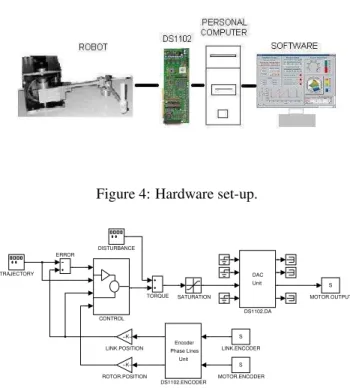
The hardware set-up is shown in Figure 4.
In this application, thedSPACE DS1102 system is used to
control the manipulator. The controller is implemented in a personal computer using theSimulink/MATLABinterface.
The controller reads the rotor angular positions in real-time from twoHewlett Packard HEDS-6010 high resolution
in-cremental encoders. Comparing the actual position and the
Figure 3: Planar flexible joint robot.
Figure 4: Hardware set-up.
TRAJECTORY
TORQUE SATURATION
−K− ROTOR.POSITION
S MOTOR.OUTPUT
S MOTOR.ENCODER −K−
LINK.POSITION
S LINK.ENCODER ERROR
Encoder Phase Lines Unit
DS1102.ENCODER
DAC Unit
DS1102.DA DISTURBANCE
CONTROL
Figure 5: Simulink implementation of the controller blocks.
reference, the controller calculates the control torque that must be sent back to the robot using the 12 bits Digital to Analog Converter outputs. The 12A PWMAdvanced Motion Controlsservo amplifier drives the necessary current to the
motor. In this application the servo amplifier is used in torque mode (voltage input to current output). Figure 5 shows the structure of the controller.
The control block represents the cascade control algorithm. Link.position and Rotor.position blocks represent the link and rotor actual positions, respectively. The Trajectory block generates the desired trajectory. The desired link positionq1d
and its derivatives, up to3rd order, are uniformly bounded.
The DAC unit and the Encoder Phase Lines unit aredSPACE
drivers that perform the digital to analog conversion and the digital interpretation of the encoder values, respectively.
6.2
Model of the Planar Flexible Joint
Robot with One Link
Using the simplified model (8), the planar robot with one link and one flexible transmission can be represented by
Iq¨1+F =K(q2−q1)
Jq¨2+K(q2−q1) =τ
(40)
where I is the inertia of the link and the load (a constant
the rotor inertia,K is the spring constant,F is the friction
torque and τ is the control torque. The inertia and spring
constant were obtained using indirect measurements. The spring constant, in particular, was obtained using a suitable experiment (Seto, 1964).
The nominal parameters for the first link of the manipulator are given in Table 1.
Table 1: First Link Parameters:
Parameter Value
I:Link Inertia (kg m2) 0.07
J :Rotor Inertia (kg m2) 0.005
K:Spring Constant (Nm/rad) 6.77
6.3
Identification of Friction Parameters
The identification of the friction parameters was done ac-cording to the procedure described in Section 5. The en-coder resolution was0.72degrees. The velocity resolution
for measuring static values was 0.1 rad/s. The static map ob-tained for the first link of the robot manipulator is shown in Fig. 6.
Using theMatlabfunctionlsqcurvefitto solve the
optimiza-tion problem (34), the static parameters are estimated as
Fs1 = 0.15Nm, Fc1 = 0.11Nm, vs1 = 0.05rad/s and
Γ21 = 0.2Nms/rad. Fig. 6 shows a non symmetric friction
with velocity, but in this paper symmetric values were used, like in (Canudas De Wit and Lischinsky, 1997).
Fig. 7 and Fig. 8 illustrate the open-loop experiment per-formed for the determination of the dynamic parameters.
Fig. 7 shows the torque input and Fig. 8 the measured an-gular position. By solving the problem optimization prob-lem 36, the dynamic parameters are estimated asΓ01= 100
−4 −3 −2 −1 0 1 2 3 4 −0.15
−0.1 −0.05 0 0.05 0.1 0.15 0.2
Constant Velocity (rad/s)
Friction (Nm)
Mesures Interpolation
Figure 6: Static map of velocity versus friction torque.
0 1 2 3 4 5 6 7 8 9 10 −1.5
−1.0 −0.5 0 0.5 1.0 1.5
Time (s)
Input Torque (Nm)
Figure 7: Open-loop experiment: input torque.
0 1 2 3 4 5 6 7 8 9 10
−0.4 −0.2 0 0.2 0.4 0.6 0.8 1
Time (s)
Position (rad)
Estimation Actual
Figure 8: Open-loop experiment: measured position and es-timated position.
Nm/rad andΓ11= 0.1Nms/rad. A simulation of the link
an-gular position using these estimated parameters is also shown in Fig. 8.
The estimated values of the 6 parameters of the LuGre model for the first link are given in Table 2.
Table 2: Estimated Parameters of the LuGre Model:
Parameter Value
Fs1 0.15 Nm
Fc1 0.11 Nm
vs1 0.05 rad/s
Γ11 100 Nms/rad
Γ01 0.1 Nm/rad
6.4
The Cascade Control Strategy
In this experiment, it is used the cascade control proposed in Section 3, adapted to the model (40) of the planar flexible joint robot considered here.
From (13) (18) and (19), the controludis given by
ud=Iq¨r1−KD1s1+ ˆF (41)
and, from (16), the control torqueτis
τ=J(¨q2d−Λ2q˙˜2)−KD2s2+K(q2−q1) (42)
Equations (41) and (42) use only accelerations and jerks of the reference signal. The control gains were chosen to obtain a response without actuator vibrations and with a sufficiently smooth control signal. Table 3 shows the controller gains.
Table 3: Controller Gains:
Gain Ke KD1 KD2 kv1 Λ1 Λ2
Value 0.001 1.0 1.0 2.0 200.0 6.0
6.5
Experimental Results
The tests were performed using two different trajectories. The link and rotor control were given by equations (41) and (42), respectively. The velocities were obtained using a filter and a numeric derivative process.
Figure 9 shows the system response using the cascade con-troller without friction compensation.
In order to outline the friction effect, Figure 10 shows the im-proved system response when using friction compensation.
0 1 2 3 4 5 6 7 8 9 10
−0.06 −0.04 −0.02 0 0.02 0.04 0.06
Time(s)
Position (rad)
Desired Actual
Figure 9: Cascade control without friction compensation.
0 1 2 3 4 5 6 7 8 9 10
−0.08 −0.06 −0.04 −0.02 0 0.02 0.04 0.06
Time (s)
Position (rad)
Desired Actual
Figure 10: Cascade control with friction compensation.
0 1 2 3 4 5 6 7 8 9 10
−1.5 −1 −0.5 0 0.5 1 1.5
Time (s)
Torque (Nm)
Torque Control Friction
Figure 11: Torque control and the estimated friction torque.
Figure 11 shows that the control torque strongly depends on the estimated friction torque.
Figure 12 shows the actual and desired link positions using a polynomial trajectory without friction compensation.
Figure 13 shows the improved system response when using the cascade controller with friction compensation.
The tracking errors for both cases are shown in Figure 14.
Figure 15 shows a faster dynamic motion experiment, which allows to better assess the performance of the cascade control algorithm with respect to the joint flexibilities. It is possible to see that the results remain good.
0 1 2 3 4 5 6 7 8 9 10 −0.08
−0.06 −0.04 −0.02 0 0.02 0.04 0.06 0.08
Time (s)
Position (rad)
Desired Actual
Figure 12: Cascade control without friction compensation.
0 1 2 3 4 5 6 7 8 9 10 −0.08
−0.06 −0.04 −0.02 0 0.02 0.04 0.06 0.08
Time (s)
Position (rad)
Desired Actual
Figure 13: Cascade control with friction compensation.
0 1 2 3 4 5 6 7 8 9 10 −0.05
−0.04 −0.03 −0.02 −0.01 0 0.01 0.02 0.03 0.04 0.05
Time (s)
Errors (rad)
WITHOUT COMPENSATION
WITH COMPENSATION
Figure 14: Tracking errors.
7
CONCLUDING REMARKS
In this paper, a systematic procedure to identify the friction model parameters and to experimentally analyse the position tracking control strategy performance, when implemented to a flexible joint robot prototype, has been presented. The pro-posed cascade control methodology uses the LuGre friction model without any assumption about the actuator’s torque
Figure 15: Cascade control compensation.
response. The convergence of the tracking errors was theo-retically proved as well as the experimental results demon-strate the effectiveness of the friction compensation. Further works will consider adaptive procedures to update the param-eters of the friction observer, the problem of design control gains to meet performance, the influence of perturbations and the study of the force control problem in robots with elastic joints.
APPENDIX A. SYMBOL NOTATION AND
MODEL PARAMETERS
In this appendix the simplified model of a flexible joint robot with friction terms and a friction force model are revisited and the parameters described in table 4 and table 5. The flex-ible robot model with the friction parameters is given by:
M(q1)¨q1+C(q1,q˙1) ˙q1+G(q1) +F =K(q2−q1)
Jq¨2+K(q2−q1) =τ
The friction force model is given by:
Table 4: Flexible Robot Model with Friction Parameters
Symbol Name
M(q1) Inertia Matrix
J=diag(J1,· · · , Jn) Rotor inertia matrix
C(q1,q˙1) Centrifuge and coriolis
terms
G(q1) Gravitational torques
K=diag(K1,· · ·, Kn) Spring matrix coefficients
τ Control inputs
q1,q˙1,q¨1 Link position, velocity and
acceleration
q2,q˙2,q¨2 Rotor position, velocity and
acceleration
F Friction force
Table 5: Friction Model Parameters
Symbol Name
z An internal state that describes the average
elastic deflection of the contact surfaces dur-ing the stiction phases
˙
z An internal state that describes the average
elastic deflection velocity of the contact sur-faces during the stiction phases
Γ0 A diagonal matrix of the stiffness coefficients
of the microscopic deformationz during the
pre-sliding displacements
Γ1 A diagonal matrix of the damping coefficients
associated toz˙
Γ2 A diagonal matrix representing the viscous
friction
REFERENCES
Al-Bender, F., Lampaert, V. and Swevers, J. (2005). The generalized Maxwell-slip model: a novel model for friction simulation and compensation, IEEE Transac-tions on Automatic Control50(11): 1883–1887.
Albu-Schäffer, A. and Hirzinger, G. (2001). Parameter iden-tification and passivity based joint control for a 7 dof torque controlled light weight robot,In proc. Interna-tional Conference on Robotics and Automation, Seoul, Koreapp. 1087–1093.
Armstrong-Hélouvry, B. (1993). Stick-slip and control in low-speed motion, IEEE Transactions on Automatic Control38(10): 1483–1496.
Brogliato, B., Ortega, R. and Lozano, R. (1995). Global tracking controllers for flexible-joint manipulators: a comparative study,Automatica31(7): 941–956.
C. Canudas de Wit, R. K. (2007). Passivity analysis of a mo-tion control for robot manipulators with dynamic fric-tion,Asian Journal of Control9(1): 30–36.
Canudas De Wit, C. and Lischinsky, P. (1997). Adaptive friction compensation with partially known dynamic model,International Journal of Adaptive Control and Signal Processing11: 65–80.
Canudas De Wit, C., Olsson, H., Åström, K. J. and Lischin-sky, P. (1995). A new model for control systems with friction,IEEE Transactions on Automatic Control
40(3): 419–425.
Canudas De Wit, C., Siciliano, B. and Bastin, G. (1996). The-ory of Robot Control, Springer - Verlag London
Lim-ited.
Corless, M. and Leitmann, G. (1991). Continuous state feed-back guaranteeing uniform ultimate boundedness for uncertain dynamic systems,IEEE Transactions on Au-tomatic Control26(5): 1139–1144.
Dupont, P. E. (1994). Avoiding stick-slip through PD control,
IEEE Transactions on Automatic Control39(5): 1094–
1097.
Fantoni, I. and Lozano, R. (2000). Adaptive stabilization of underactuated flexible-joint robots using an energy approach and min-max algorithms, In Proceedings of the American Control Conferencepp. 2511–2512.
Gandhi, P. S., Ghorbel, F. H. and Dabney, J. (2002). Model-ing, identification, and compensation of friction in har-monic drives,Proc. of the 41st IEEE Conf. on Decision and Control.
Ghorbel, F. and Spong, M. W. (2000). Integral mani-folds of singularly perturbed systems with application to rigid-link flexible-joint multibody systems, Interna-tional Journal of Nonlinear MechanicsJune(34): 133–
155.
Gomes, S. C. P. and Santos da Rosa, V. (2003). A new approach to compensate friction in robotic actu-ators, Robotics and Automation, 2003. Proceedings. ICRA’03. IEEE International Conference on 1: 622–
627.
Guenther, R. and Perondi, E. (2002). The pneumatic posi-tioning system cascade control with friction compen-sation, In Proceedings of the Congresso Brasileiro de Automaticapp. 100–106.
Guenther, R. and Perondi, E. (2004). O controle em cas-cata de sistemas pneumáticos de posicionamento, Re-vista SBA Controle e Automação15(2): 149–161.
Guenther, R., Perondi, E., De Pieri, E. R. and Valdiero, A. C. (2006). Cascade controlled pneumatic position-ing system with lugre model based friction compen-sation, Journal of the Brazilian Society of Mechanical Sciences and Engineering,28(1): 48–57.
Huang, L., Ge, S. S. and Lee, T. H. (2006). Position/force control of uncertain constrained flexible joint robots,
Mechatronics16(2): 111–120.
Jeon, S. and Tomizuka, M. (2005). Limit cycles due to fric-tion forces in flexible joint mechanisms,Advanced In-telligent Mechatronics. Proceedings, 2005 IEEE/ASME International Conference onpp. 723–728.
Kokotovic, P. and Sussmann, P. (1989). A positive real con-dition for global stabilization of nonlinear systems, Sys-tems and Control Letters13(2): 125–133.
Lischinsky, P., Canudas-De-Wit, C. and Morel, G. (1999). Friction compensation for an industrial hydraulic robot,
IEEE Control SystemsFeb.: 25–32.
Lozano, R., Valera, A., Albertos, P. and Arimoto, S. (1997). PD control of robot manipulators considering joint flex-ibility actuators dynamic and friction,In Proceedings of the American Control Conferencepp. 2638–2641.
Nicosia, S. and Tomei, P. (1988). On the feedback lineariza-tion of robots with elastics joints, In Proceedings of the IEEE International Conference on Robotics and Au-tomationpp. 180–185.
Nicosia, S. and Tomei, P. (1992). A method to design adap-tive controllers for flexible joint robots,In Proc. IEEE Int. Conf. on Robotics and Automationpp. 701–706.
Ramirez, A. R. G., De Pieri, E. R. and Guenther, R. (2002). Experimental study applied to an industrial robot by us-ing variable structure controllers and friction compen-sation, Journal of the Brasilian Society of Mechanical SciencesXXIV(4): 302–309.
Ramirez, A. R. G., De Pieri, E. R. and Guenther, R. (2003). Controle em cascata de um manipulador robótico com um elo e uma transmissão flexível, Revista SBA Cont-role e Automação14(4): 393–401.
Readman, M. C. (1994).Flexible Joint Robots, CRC Press.
Seto, W. (1964).Theory and Problems of Mechanical Vibra-tions, McGraw Hill.
Spong, M. W. (1987). Modelling and control of elastic joint robots,ASME, Transactions: Journal of Dynamic Sys-tems, Measurement, and Control109: 310–319.
Spong, M. W. and Vidyasagar, M. (1989). Robot Dynamics and Control, Prentice Hall, Inc., New Jersey.
Tomei, P. (1991). A simple PD controller for robots with elastic joints,IEEE Transactions on Automatic Control
36(10): 1208–1213.
Tomei, P. (2000). Robust adaptive friction for tracking con-trol of robot manipulators,IEEE Transactions on Auto-matic Control45(11): 2164–2169.
Wang, Z. and Khorrami, F. (2000). Robust trajectory track-ing for manipulators with joint flexibility via backstep-ping,In Proceedings of the American Control Confer-encepp. 2849–2853.