494
Revista da Sociedade Brasileira de Medicina Tropical 48(4):494-497, Jul-Aug, 2015
http://dx.doi.org/10.1590/0037-8682-0013-2015
Short Communication
Corresponding author: Dr. Edson Zangiacomi Martinez. Deptº de Medicina Social/ FMRP/USP. Av. Bandeirantes 3900, Monte Alegre, 14049-900 Ribeirão Preto, São Paulo, Brasil.
Phone: 55 16 3602-2569 e-mail: [email protected] Received 13 January 2015 Accepted 30 March 2015
Description of continuous data using bar graphs:
a misleading approach
Edson Zangiacomi Martinez
[1][1]. Departamento de Medicina Social, Faculdade de Medicina de Ribeiro Preto, Universidade de São Paulo, Ribeirão Preto, São Paulo, Brasil.
ABSTRACT
Introduction: With the ease provided by current computational programs, medical and scientifi c journals use bar graphs to describe continuous data. Methods: This manuscript discusses the inadequacy of bars graphs to present continuous data. Results: Simulated data show that box plots and dot plots are more-feasible tools to describe continuous data. Conclusions: These plots are preferred to represent continuous variables since they effectively describe the range, shape, and variability of observations and clearly identify outliers. By contrast, bar graphs address only measures of central tendency. Bar graphs should be used only to describe qualitative data.
Keywords: Biostatistics. Descriptive statistics. Medical research.
Over the decades, many authors have used bar graphs to describe continuous data(1). The height of the bars in these graphs
indicates a measure of central tendency (mean or median) of the data, while error bars describe a measure of dispersion (standard deviation) or precision (standard error). These graphs have become quite popular with the ease provided by some current computer programs. Despite their wide use, bar graphs have fostered a misleading approach to describe continuous data, while traditional tools such as box plots and dot plots are more suitable for this purpose. Bar graphs do not provide useful information about the behavior of data, such as skewness, range, and presence of atypical values (outliers). They only describe the position of the mean (or median) and dispersion around this measure.
The box plot, also called box-and-whiskers plot, was introduced by the American mathematician John Wilder Tukey (1915-2000) as a practical method to describe groups of numerical data based on their quartiles and extreme values(2).
When represented vertically, the box plot displays a rectangle
(the box) whose base and top represent the position of the fi rst
(Q1) and third (Q3) quartiles, respectively. A band inside the rectangle describes the second quartile (the median). The height of the rectangle then represents the inter-quartile range (IQR), and can be interpreted as a measure of data spread. To complete the graph, two vertical lines connect the third quartile to the
highest value and the fi rst quartile to the lowest value. A practical
method to detect potential outliers is to identify values above
Q3 + 1.5 IQR and bellow Q1 – 1.5 IQR in the plot. Outliers are represented by points (or other symbols), and vertical lines connect the third quartile to the highest point below Q3 + 1.5
IQR and the fi rst quartile to the lowest value above Q1 – 1.5 IQR.
This is the standard form of a box plot, but since its introduction by Tukey, many alternative forms have been proposed(3) (4). The
dot plot can be used to describe small sizes, since the box plot requires a sample size of at least 5 to be adequate.
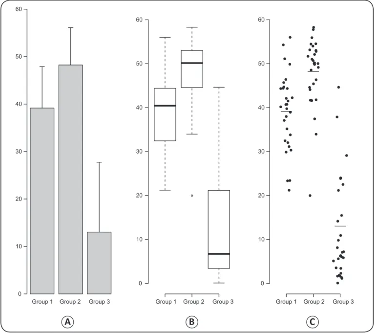
For example, we simulated data on a continuous variable with different means, dispersion, and skewness among three groups. For each group, we simulated samples of size n = 30.
In the fi rst and second groups, the variable follows a normal
distribution with population means 40 and 50, respectively, and standard deviations 8 and 6, respectively. In the third group, the variable follows an asymmetric gamma distribution with population mean 12.5. Figure 1A shows a bar graph with standard deviation bars describing these data (height of the bars indicates the means), while Figure 1B and Figure 1C show box plots and dot plots, respectively, where vertical lines overlapping the points represent sample means. We note that the bar graph (Figure 1A) provides no information about the range of observed data (minimum and maximum values) or the presence of outliers. In addition, the bar graph cannot describe the shape of the data distribution. Evidence of data symmetry or non-symmetry and information about the presence of outliers are crucial to the choice of an appropriate statistical method of analysis. For example, analysis of variance (ANOVA) and t-tests involve statistics whose asymptotic distributions are well approximated by known density probability functions (such as Student’s t or Snedecor’s F). However, these approximations cannot be satisfactorily achieved when the data distribution is skewed(5), and the results obtained from these analyses can be
consequently spurious. Outlier values can strongly infl uence
495 Martinez EZ - Description of continuous data using bar graphs
0 10 20 30 40 50 60
0 10 20 30 40 50 60
0 10 20 30 40 50 60
Group 1 Group 2 Group 3 Group 1 Group 2 Group 3 Group 1 Group 2 Group 3
A
B
C
FIGURE 1 - Data are shown for three simulated samples (n = 30) from normal (Groups 1 and 2) and gamma (Group 3) distributions. A: Bar graphs with standard deviation bars are inadequate. B: Box plots adequately describe the data distribution and highlight an outlier. C: Dot plots are also adequate to describe data. The horizontal lines in this graph represent the means.
is small. However, box plots (Figure 1B) and dot plots (Figure 1C) adequately describe the range of observations, satisfactorily present the shape of the data distribution, and clearly demonstrate the presence of outliers. The layout of Figure 1A is not the same as that of Figure 1B or Figure 1C. Box plots and dot plots can easily be obtained with the aid of packages such as R, Stata, SPSS, or SAS. However, the use of SAS and R software requires some knowledge of programming language, but Stata and SPSS are user-friendly software packages
that allow a beginner to create them with relative ease. The fi gures
in this article were prepared using R, a software available free
of charge at http://www.r-project.org/. The R codes for drawing
the graphs are omitted here, but are available with the author.
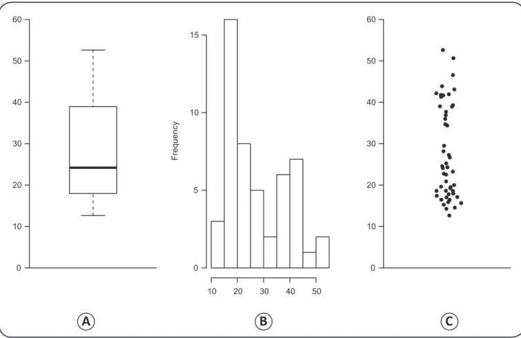
A disadvantage of the box plot is that it cannot clearly describe the distribution of data with more than one mode. This situation is quite common when dealing with mixtures of two or more different populations. For example, the distribution of anthropometric data from a sample of both genders usually present different shapes for men and women. Figures 2A, Figure 2B, and Figure 2C show, respectively, a box plot, a histogram, and a dot plot for simulated data from a variable that follows a mixture of two normal distributions with means 20 and
40 and standard deviations 3 and 5. The sample size was fi xed at 30 and 20 for the fi rst and second components, respectively. We
496
Rev Soc Bras Med Trop 48(4):494-497, Jul-Aug, 2015
0 10 20 30 40 50 60
Frequenc
y
10 20 30 40 50 0
5 10 15
0 10 20 30 40 50 60
A
B
C
FIGURE 2 - Box plots cannot clearly describe multimodal distributions. A: Box plot for a sample from a random variable that follows a mixture of two normal distributions. The bimodality is not visible in this graph. B: A histogram for these data. The bimodality is
now visible in this graph. C: A dot plot for these data. The display of two clouds of points in this fi gure suggests a bimodal distribution.
options to highlight the shape of data. However, dot plots allow
two or more groups in a single fi gure to be compared, but this can be diffi cult when using a histogram. The display of two clouds
of points (Figure 2C) exemplifi es how this fi gure is capable of describing the behavior of data.
Criticism of the use of bar graphs to describe continuous data can also be found in an article by Krzywinski and Altman (1), who
argue that box plots are a rather more communicative way to show sample data. Strongly discouraging the use of bar plots with error bars, the authors state that this misleading visual approach has unfortunately been more widely used in the medical literature than have box plots. In addition, the bar itself reportedly encourages the visual perception that the respective mean is related to its height rather than the position of its top (1).
Streit and Gehlenborg(6), too, provide useful commentaries on
the use of bar graphs.
As discussed by Cumming et al.(7), some fi gures with error
bars can, if used properly, give useful information about the data. These authors warn that it is necessary to distinguish between descriptive and inferential bars, given that they provide different
information, such as confi dence intervals, standard errors,
standard deviations, or simply an amount of spread between
the extremes of data. Descriptive bars address the variability of sample data, while inferential bars are related to the precision of the result. It is important to note that bars expressing standard deviations are not properly interpreted as error bars since the standard deviation is a measure of the sample variability around the sample mean, instead of a precision measure in relation to the true value of the population mean. For these reasons, various authors(8) (9) have argued about the importance of including
legends or subtitles on their fi gures describing the meaning of
the bars. Other details about the adequate use of error bars are presented by Altman(10).
In conclusion, the choice of an appropriate graphical tool for data description should not be made according to the convenience
offered by computer programs or even infl uenced by the aesthetic of the fi gure. It is important that data visualization consider the
497
ACKNOWLEDGMENTS
I am grateful to the anonymous reviewers of this journal for
their constructive comments and suggestions.
REFERENCES
The author declare that there is no confl ict of interest. CONFLICT OF INTEREST
1. Krzywinski M, Altman N. Visualizing samples with box plots. Nat Methods 2014; 11:119-120.
2. Tukey JW. Exploratory Data Analysis. Reading: Addison-Wesley Publishing Co; 1977.
3. McGill R, Tukey JW, Larsen WA. Variations of box plots. Am Stat 1978; 32:12-16.
4. Hintze JL, Nelson RD. Violin plots: a box plot-density trace synergism. Am Stat 1998; 52:181-184.
5. Bland JM, Altman DG. The use of transformation when comparing two means. BMJ 1996; 312:1153.
6. Streit M, Gehlenborg N. Bar charts and box plots. Nat Methods 2014; 11:117.
7. Cumming G, Fidler F, Vaux DL. Error bars in experimental biology. J Cell Biol 2007; 177:7-11.
8. Vaux DL. Error message. Nature 2004; 428:799.
9. Belia S, Fidler F, Williams J, Cumming G. Researchers misunderstand confi dence intervals and standard error bars. Psychol Methods 2005; 10:389-396.
10. Altman DG. Statistics and ethics in medical research, VI. Presentation of results. Br Med J 1980; 281:1542-1544.