Volume 31, Issue 2
Sluggish information diffusion and monetary policy shocks
Orlando Gomes
ISCAL / Lisbon Politechnique Institute and Business Research Unit / ISCTE-LUI
Vivaldo M. Mendes Business Research Unit / ISCTE-LUI
Abstract
The sticky-information model appeared in order to offer a more empirically consistent view on the effects of monetary policy than the one provided by the benchmark sticky prices setup. Such inattentiveness framework was built on the assumption that current decisions are mainly based on past expectations about the current state of the economy. In this note, we propose an explanation for information stickiness that goes beyond the simple idea of infrequent updating of expectations. The suggestive new feature is that contemporaneous decisions will depend on a process of information diffusion that is triggered by the relation between two rational players: the profit maximizing media industry and the private agents, who seek information in order to update prices.
The comments and suggestions of an anonymous referee are gratefully acknowledged. The usual disclaimer applies.
Citation: Orlando Gomes and Vivaldo M. Mendes, (2011) ''Sluggish information diffusion and monetary policy shocks'', Economics Bulletin, Vol. 31 no.2 pp. 1275-1287.
Submitted: Feb 06 2011. Published: April 27, 2011.
1
Introduction
This note reinterprets the sticky-information approach to monetary policy pioneered by Mankiw and Reis (2002). In the original framework, information is sticky because …rms are heteroge-neous in what concerns the time moment in which they collect information in order to recompute optimal prices. The proposed mechanism, based on an adjustment assumption according to which each …rm has a same probability of being one of the …rms updating information indepen-dently of the timing of the last update, implies that current prices are a weighted average of past expectations on the contemporaneous optimal price level. However, this stickiness framework is silent in what concerns the process through which individuals acquire information in speci…c time moments, i.e., the model postulates that information disseminates slowly throughout the population, without furnishing any clue on why this happens. Clearly, a black box exists in this reasoning and one needs to look inside it to gain further knowledge on the economic responses to monetary shocks.
Relying on the literature on technology di¤usion, and more speci…cally on the analysis of Mukoyama (2006), we adapt the innovation di¤usion mechanism to a setup of information dissemination where a permanent feedback between two entities exists: …rms in the media industry intend to produce appealing and informative news in order to maximize audiences; the population desires to access relevant information and to remain attentive in order to decide about price updates. From this intertemporal interaction relation emerges an S-shaped di¤usion process: on a …rst phase, the curve relating to the number of individuals accessing some new information exhibits increasing marginal increments; on a second stage, such increments become decreasing. At the end of the information dissemination process, a given share of the agents in the market or the whole market have accessed the new information.
The appealing set of results that the analysis will furnish relates to the ability of the di¤usion setup in reproducing, for given parameter values, the same perturbations on in‡ation and output trajectories arising from various types of monetary policy changes that one …nds in the information stickiness framework. Thus, the analysis adds value to the sticky information literature by presenting a reasonable explanation on how di¤erences on the timing of information acquisition arise.
A work that has common traits with ours is the one by Carroll (2006). Such contribution also assumes that expectations are formed over information obtained through the news media. The main di¤erence is that the referred paper models information dissemination exogenously as an infectious disease or an epidemic, without establishing the foundations under which information di¤uses, which is precisely what we intend to do.
The note is organized as follows. Section 2 reviews the main features of the sticky-information model and the policy experiments developed in Mankiw and Reis (2002). Section 3 introduces the information di¤usion mechanism. In section 4 information di¤usion is attached to the for-mation of the next period’s price level. Section 5 will then address the dynamics of the model, highlighting that the obtained results can accurately mimic the ones in the sticky-information formulation. Finally, section 6 concludes.
2
The Sticky-Information Setup
We consider an economy with many monopolistically competitive …rms. The pro…t maximiza-tion behavior of the …rms implies the following desired price for each …rm (i.e., the price that maximizes pro…ts at each time moment),1
pt = pt+ yt (1)
In equation (1), pt and yt represent, respectively, the price level and the output gap (both measured in logs). Parameter > 0 is a measure of real rigidities; it indicates the degree of sensibility of desired prices relatively to the real performance of the economy. The intuition is straightforward: expansion phases of the business cycle imply increases in demand and the corresponding desire of …rms in rising prices; recessions will lead to a desired contraction of prices relatively to the existing price level.
The sticky information model assumes that only a share 2 (0; 1) of …rms in the market will update prices at each time moment, following a Poisson distribution. Thus, the price level at time t will correspond to
pt= 1 X
j=0
(1 )jEt jpt (2)
Equation (2) tells us that all …rms intend to set prices at the desired level, however they collect information and form expectations about such desired price at di¤erent moments in the past. This equation can be transformed into a Phillips curve, where a positive contemporaneous relation between output and in‡ation becomes evident:
t= 1 yt+ 1 X j=0 (1 )jEt 1 j( t+ gt) (3)
with t:= pt pt 1 the in‡ation rate and gt:= yt yt 1 the growth rate of the output gap. To address the dynamics of in‡ation and output, one needs to close the model with an equation representing aggregate demand. Letting mt denote money supply or, more broadly, the whole set of factors capable of shifting aggregate demand, one establishes the relation
mt= pt+ yt (4)
The e¤ects of monetary policy will be addressed by imposing exogenous changes to mt, in order to explore the corresponding impact over t and yt. To make such relation more transparent, replace yt in (3) by the di¤erence between money and prices (according to (4)), and apply …rst-di¤erences, to obtain
t+1 = m + (1 ) t+ (1 ) 1 X j=0 (1 )jEt+1 j( t+1) (5) (1 ) 1 X j=0 (1 )jEt j( t)
1We avoid presenting the details of the optimization problem not only because of space limitations but also
because this is a trivial problem in the literature. See Blanchard and Kiyotaki (1987) for details.
Expression (5) is a rule translating the motion in time of the in‡ation rate as the result of eventual changes in monetary policy (or demand conditions). The term mcorresponds to the rate of growth of money supply, mt+1 mt, which can be considered constant between monetary policy changes. Note that under a purely deterministic environment with expectations formed under perfect foresight, the model (i.e., equation (5)) may be reduced to relation
t+1 = m + (1 ) t (6)
Because 2 (0; 1), it is straightforward to characterize the dynamics of the model: the in‡ation path is stable, implying that for any 0, the system will converge to the steady state outcome = m. Parameter will represent the velocity of convergence; the less attentive …rms are, the slower will be the convergence towards the monetary steady state.
Relatively to the speci…ed macro framework, Mankiw and Reis (2002) propose the following policy experiments:
(i) Permanent negative change in the level of aggregate demand, not known with antic-ipation. A 10% fall in the value of mt is considered at time t = 0. Previously to t = 0, mt = ln(0:9) and for t 0, mt becomes equal to zero. Evaluating this experiment resorting to (5), one regards that in‡ation gradually falls but after a given length of time recovers its ini-tial value. This policy measure is also contractionary in the sense that it produces a temporary fall in the output gap.
(ii) Unanticipated fall in the rate of money growth. A 2.5% per period fall in the value of mt is assumed for t < 0; for t 0, the rate of growth of the money supply becomes equal to zero. This experiment reveals that the sticky information setting will again imply a gradual reduction in in‡ation, resting in the long run at the new level of demand growth (recall that in the steady state = m). The output gap su¤ers a fall after the shock but its value returns gradually to zero.
(iii) The fall in the rate of money growth is the same as in the previous experience, however now such policy change is announced 8 periods before it e¤ectively occurs (at t = 8). In this case, in‡ation falls but in a less pronounced way than in the surprise disin‡ation case, and the contractionary e¤ect on the output gap is also less pronounced.
(iv) The change in money supply is modelled as a …rst-order autoregressive process: mt= mt 1+"t, with j j < 1 and "tan eventual perturbation over the growth of money supply. The selected values are = 0:5and "0 = 0:007("t6=0 = 0). Again, a contractionary e¤ect on output and a fall in the in‡ation rate occur after the shock with the maximum e¤ect happening only after some time periods. It is evident in this and in the previous experiments which is the main consequence of the formalized information sluggishness setup: an inertia e¤ect arises, making the impact of monetary policy having its maximum strength some time after the disturbance takes place.
All the four experiments are developed by taking time periods of a quarter of a year and by assuming the following parameter values: = 0:1 (the degree of real rigidities is not too signi…cant) and = 0:25(…rms update information once a year, on average).
3
The Process of Information Di¤usion
Consider an economy where a single source of information exists (a news agency). After a given economic event (e.g., a shock on demand), a large number of media …rms (newspapers, radios
and TV stations) will resort to the information originating on the agency to produce news on the assumed speci…c subject. The number of media …rms is Z. Some of these companies will produce accurate, self-contained and easily understandable information; others will convey news with some sort of inaccuracy or di¢ cult to understand from the point of view of the interested audience. Thus, at a given time moment t there are Xt=
Z P i=1
xi
t imprecise news on the event, if one de…nes
xit= 1if the news are inaccurate / di¢ cult to understand;
0if the news are rigorous and precise. ; i = 1; 2; :::; Z:
The number of agents attentive to the news at each time moment is Nt; the medium chosen to access the news is selected at random from set Z, with this random choice being independent across time and across individual agents in the economy. When the news are inaccurate or di¢ cult to understand, this is reported back to the media (today this has become extremely common; the public interacts with the media through various channels: on-line discussion forums, e-mail messages and letters to the news o¢ ces, public opinion programs on radio and TV). The information producer will then improve the quality / readability of the contents and generate more accurate and reader / listener / viewer - friendly news that will reach a broader audience.2
Let qt := (Z Xt)=Z de…ne the degree of news informativeness; if qt = 0, all news on the subject are uninformative; on the other extreme, qt = 1 implies that the news are completely understandable and readily accessible to the whole of the potential audience. We also de…ne nt := Nt=Z as the number of individual agents accessing, on average, the news of a speci…c single information source (the number of agents attentive to the contents of a speci…c medium). If, at moment t, no one accesses the contents of the media company i and they contain errors or are uninformative, this implies that the errors are not corrected and the information remains uninformative at time t + 1. Thus, we can establish the probability
Pr xit+1= 1j xit = 1 = 1 1 Z
Nt
or, considering simultaneously all the news that are uninformative, E[Xt+1jXt] = Xt 1
1 Z
Nt
From the previous expectation, one realizes that E[qt+1jqt] = 1 (1 qt) 1
1 Z
Znt
By assuming Z ! 1 (i.e., a very large number of news media exists) and noticing that lim
Z!1 1 1 Z
Znt
= exp( nt), we can present the following deterministic di¤erence equation for
2We focus our attention on the receivers of the news and on how they react to incentives. Relatively to
the producers of the news, media …rms, we implicitly consider that they have an advantage in re…ning the quality of their output in order to maximize audiences. The maximization of the number of clients is a crucial feature of the information related industries, since the respective production process is typically associated to zero marginal costs and, thus, pro…t maximization requires placing special attention on the revenues side.
the motion of the news informativeness variable:
qt+1= 1 (1 qt) exp( nt); q0 given. (7)
Equation (7) establishes an intuitive relation between the informativeness of news and the number of agents accessing the news conveyed by each media …rm. As one should expect, @qt+1=@nt = (1 qt) exp( nt) > 0, i.e., the larger the number of agents accessing the news of given media, the faster dubious contents on the news are reported and the faster the qual-ity of the news is improved (for the speci…c equation (7), the qualqual-ity of news increases ex-ponentially with the number of individuals accessing news). Note also that @2q
t+1=@n2t = (1 qt) exp( nt) < 0; this derivative indicates that the rate of improvement in the news will be subject to decreasing marginal returns: as nt increases it becomes harder to …nd new ’bugs’ on the conveyed information and therefore the quality improves at a slower pace.
The above reasoning indicates how the number of individuals accessing news in‡uences the quality of news. We now need to look at the opposite direction: how the improved quality allows for an increase of agents being attentive to that speci…c news. It seems evident that the higher is the quality level of the news, the more agents will want to access them. To formalize this idea, consider that the utility of news for an agent ` is given by u`
t = u`(1 (1 qt)), with u` > 0a parameter that will assume di¤erent values across agents; we also consider > 0. The presented expression translates the idea that the larger is the quality of news, the larger will be the degree of utility agent ` withdraws from the news. Let the cost of acquiring news be c. The news will be acquired if u`
t c. If u` follows a Pareto distribution of the type D(x) = 1 b=x with b a parameter such that x b, then the number of agents accessing the news at time t is:
nt= 1 D
c 1 (1 qt)
=en(1 (1 qt))
with en := b=c the maximum number of agents that can access a given news source. The larger is the overall quality of the news, the larger will be the share of individuals accessing a given medium, relatively to its potential demand: @nt=@qt = en > 0. Replacing qt by nnet + k1 in equation (7), one obtains the following rule of motion for the number of agents accessing news of a given source:
nt+1=en (en nt) exp( nt); n0 given. (8)
4
Price Dynamics under Information Di¤usion
In this section, we explain how the information di¤usion process can be used in order to address the macroeconomic response to demand / monetary policy shocks. Agents that have already accessed the information on the shock and have understood it will form expectations pIt+1 := Etpt+1 = pt+1 (expectations are rational) for the price level in t + 1, with pt the desired price de…ned in equation (1). The agents that do not have yet accessed or processed the news on the change of demand conditions will select a price that is equal to the previous price plus the growth rate of money supply that existed previously to the disturbance. Let mj
t<0 be this
growth rate with t< 0 the set of information known prior to the announcement of the shock. Type II agents will select the following price for t + 1: pIIt+1:= pt+ mj t<0.
Therefore, prices at t + 1 will be given by a weighted average: pt+1 = nt+1 en pt+1+ en nt+1 en pt+ mj t<0 (9)
Given the de…nition of desired price in equation (1), one is able to rewrite (9) under the form of a Phillips curve,
t+1 =
nt+1 en nt+1
yt+1+ mj t<0 (10)
The Phillips curve in (10) reveals the usual positive contemporaneous relation between income / output and the in‡ation rate. Note that the larger is the number of agents that already accessed the information, the larger is the impact of the output gap over price changes. In the limit case nt+1=en, we are in the steady-state position, where we regard that y = 0.
Combining (10) with the market clearing condition (4) and applying …rst di¤erences, one obtains the following expression re‡ecting the motion in time of the in‡ation rate:
t+1 = 1 en (1 )nt+1 (11) (en nt)nt+1 nt t+ nt+1 mj t 0 en(n t+1 nt) nt mj t<0
The main point this paper wants to stress is that in‡ation di¤erence equation (11) combined with the information di¤usion rule (8) is capable of generating the exact same results as the sticky-information model when the same policy experiments are undertaken. Before addressing such experiments in the next section, note the main features of system (8)-(11):
1. The steady-state of the system is (n ; ) = (en; mj
t 0), i.e., all agents have access,
sooner or later, to the relevant information about the policy measure and, in the long-run, in‡ation will be equal to the rate of growth of money supply that prevails after the shock.
2. Considering exclusively a deterministic interpretation of the referred system, one encoun-ters a local stability result. To con…rm this, compute derivatives in the vicinity of the steady-state for equation (11),
@ t+1 @ t (n ; ) = 0; @ t+1 @nt (n ; ) = (1 ) exp( en) 1 + en en mj t 0 exp( en) 1 en mj t<0
The following linearized system characterizes the local dynamics of the model, nt+1 en t+1 mj t 0 = " exp( en) 0 @ t+1 @nt (n ; ) 0 # nt en t mj t 0
The eigenvalues of the Jacobian matrix in the above system are e1 = exp( en) and e2 = 0. Because jeij < 1; i = 1; 2, for any positive en, stability holds.3
3Local stability indicates that for any
0in the vicinity of , the trajectory in time followed by the in‡ation
rate is a trajectory of convergence towards . Furthermore, since nt2 (0; en), equation (11) also provides the
information that the basin of attraction of the steady-state is the whole universe of potential levels of tand,
thus, stability is global. Any numerical example can con…rm this.
5
Policy Experiments
As mentioned earlier, the policy experiments we undertake are exactly the same ones as in Mankiw and Reis (2002). We consider the same level of real rigidities, = 0:1, and now the degree of sticky-information no longer applies. Instead, one needs to de…ne the value of en and the initial value n0. Recall en de…nes the percentage of individuals that potentially access a given information source, while n0 is the percentage of agents that e¤ectively resort to the information source in the precise moment in which the news about the monetary policy measure are generated for the …rst time (the group of exceptionally attentive agents). We takeen = 0:22 and n0 = 0:05. Under a complete di¤usion process, nt will converge from n0 to en; for the selected values, the convergence process is relatively fast: after 20 periods the information has asymptotically reached all the population; after 6 periods, 50% of the population has already accessed and processed the news. If one is considering quarterly data, this implies that it takes one and a half year for the monetary policy measure to be spread by one half of the price setting agents.
We recover the policy experiments:
(i) Non anticipated 10% fall in the level of aggregate demand. Figure 1 presents the e¤ects of such shock, occurring at time t = 0, for the selected parameter values.4 Panel A concerns the impact of the perturbation over the output gap (the shock has an evident contractionary e¤ect); panel B respects to the reaction of the in‡ation rate (the strongest e¤ect is felt after 9 to 10 periods, given the sluggishness introduced by the di¤usion process). Once the disturbance takes place, the di¤usion of information begins from n0 = 0:05 toen = 0:22; this process obeys to the motion rule (8), i.e., to the S-shaped process of information dissemination. The information di¤usion process that begins with the disturbance occurring in the economy implies that it will take time for all the agents to access the new information, what justi…es the shape of both the output gap and the in‡ation rate trajectories.
(ii) Non anticipated fall in the rate of money growth at date t = 0, from 2.5% per quarter to 0%. For this case, …gure 2 illustrates the impact over output and in‡ation. In‡ation falls from the …rst to the second equilibrium point, but with this process involving a contractionary e¤ect: in the transition phase, in‡ation falls below zero. The output gap also falls below zero but it returns precisely to this same value in the long-run. The di¤usion process is the same and it begins at the same moment as in the …rst experiment.
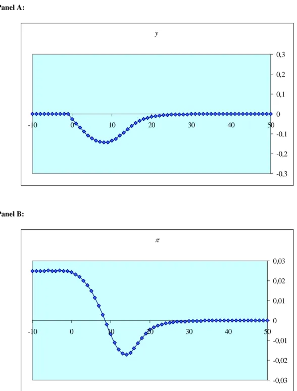
(iii) Anticipated fall in the rate of money growth, announced at t = 8 to occur at t = 0 (again, the change is from 2.5% growth per quarter to 0% growth per quarter). Figure 3 reveals that the fall in the output gap is less pronounced than in the previous case, while the contractionary e¤ect over the price level is again felt only after t = 0 but with a reduced impact. In this case, we are considering the exact same di¤usion process as in the previous experiments, but now it starts at t = 8, instead of beginning at t = 0.
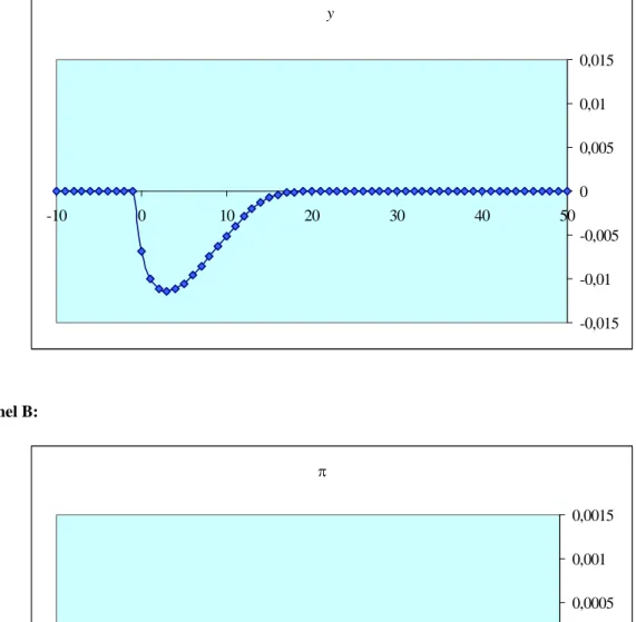
(iv) Finally, we consider an AR(1) process for the money supply evolution in time with a negative shock ("0 = 0:007) occurring at t = 0. In this case, the economy will again experience a relatively sluggish decline in both the output gap and the in‡ation rate and a re-establishment of the equilibrium after around 20 periods. Again, the shock triggers the same type of di¤usion process as in the previous cases, and it will be this process that shapes the evolution of yt and
t observed in …gure 4.
4All …gures are presented at the end of the paper.
6
Conclusion
Given zero marginal costs, …rms in the media industry will have an incentive to maximize audiences. They achieve this goal through a process of re…nement of the quality of news. Such process allows price setting …rms to access relevant economic information that they can use to update their expectations. Because agents are heterogeneous with respect to the capacity to absorb information, any policy disturbance a¤ecting the economy will imply a gradual departure from the steady-state. The steady-state is recovered as price-setters gradually access news and update expectations accordingly. An inertia e¤ect then characterizes the response of the economic system to shocks that will eventually occur.
Figures 1 to 4 are identical to the ones presented in Mankiw and Reis (2002), for the exact same policy experiments. Thus, it is reasonable to conclude that information stickiness can be explained through a process of information dissemination, which arises from the coexistence in the society of agents requiring information and media companies that desire to maximize revenues for a given cost structure.
References
[1] Blanchard, O. and N. Kiyotaki (1987). "Monopolistic Competition and the E¤ects of Ag-gregate Demand." American Economic Review 77, 647-666.
[2] Carroll, C. D. (2006). “The Epidemiology of Macroeconomic Expectations.” in L. Blaume and S. Durlauf (eds.), The Economy as an Evolving Complex System III, Oxford: Oxford University Press.
[3] Mankiw, N. G. and R. Reis (2002). "Sticky Information versus Sticky Prices: a Proposal to Replace the New Keynesian Phillips Curve." Quarterly Journal of Economics 117, 1295-1328.
[4] Mukoyama, T. (2006). "Rosenberg’s ’Learning by Using’and Technology Di¤usion." Journal of Economic Behavior and Organization 61, 123-144.
Panel A: y -0,15 -0,1 -0,05 0 0,05 0,1 0,15 -10 0 10 20 30 40 50 Panel B: π -0,012 -0,007 -0,002 0,003 0,008 -10 0 10 20 30 40 50 1284
Fig. 2 – Effects of policy experiment II Panel A: y -0,3 -0,2 -0,1 0 0,1 0,2 0,3 -10 0 10 20 30 40 50 Panel B: π -0,03 -0,02 -0,01 0 0,01 0,02 0,03 -10 0 10 20 30 40 50 1285
Panel A: y -0,3 -0,2 -0,1 0 0,1 0,2 0,3 -10 0 10 20 30 40 50 Panel B: π -0,03 -0,02 -0,01 0 0,01 0,02 0,03 -10 0 10 20 30 40 50 1286
Fig. 4 – Effects of policy experiment IV Panel A: y -0,015 -0,01 -0,005 0 0,005 0,01 0,015 -10 0 10 20 30 40 50 Panel B: π -0,0015 -0,001 -0,0005 0 0,0005 0,001 0,0015 -10 0 10 20 30 40 50 1287