Computational procedures for nonlinear analysis of frames with semi-rigid connections

Computational procedures for nonlinear analysis of frames with

semi-rigid connections

Leonardo Pinheiroa and Ricardo A. M. Silveirab,∗

a

Civil Engineering Program, Federal University of Rio de Janeiro – COPPE/UFRJ Ilha do Fund˜ao – Cidade Universit´aria, s/n, Centro de Tecnologia, Bloco B, Sala B 101 21945-970, Rio de Janeiro – RJ –

Brazil

b

Civil Engineering Graduate Program – PROPEC

Department of Civil Engineering, Federal University of Ouro Preto – UFOP Morro do Cruzeiro – Campus Universit´ario, s/n, 35400-000, Ouro Preto – MG – Brazil

Abstract

This work discusses numerical and computational strategies for nonlinear analysis of frames with semi-rigid connections. Initially, the formation of the nonlinear problem is an-alyzed, followed by the necessary computational approaching for its solution. After that, the matricial formulations and the mathematical modeling of flexible connections, as well as the insertion of the nonlinear process, are presented. Moreover, the necessary procedures for characterization of semi-rigid beam-column elements, the modified stiffness matrix, the inter-nal forces vector and the updating of the connection stiffness along the incremental-iterative process are approached and illustrated through the text. In order to verify the success of the implementations and the considered algorithms, the results for some types of frames considering semi-rigid joints are compared with those supplied by literature. Some consid-erations and conclusions about the computational implementations and results obtained are presented at the end of this work.

Keywords: frames, semi-rigid connections, finite element method, hybrid element, nonlinear analysis, stiffness matrix.

1 Introduction

types, it is commonly recommended, due to the advance in solution methods, the expansion of computational memory, and, more directly, the drastic decline in computation costs, that nonlinear analyses are taken into account to investigate the behavior of structures under unusual load conditions.

Another recurrent fact in conventional projects and structural analysis is the consideration that the connections between beam and column are perfectly rigid or ideally pinned. The first hypothesis implies that the angle between adjoining members remains unchanged, what results in the assumption that the relative stiffness of connections between such elements is very large. Otherwise, the second hypothesis results in the condition that no moment is transmitted from beam to column, in which it is assumed that joint stiffness is very small when compared with one of the connected members. However, such hypotheses are practically unrealizable. Several experiments have demonstrated that, in fact, the connections are in an intermediate level between the extreme conditions of totally rigid and ideally pinned, what means the joints have a finite degree of flexibility. Therefore, the connections are, in practice, semi-rigid. Moreover, they have a nonlinear behavior that can be one of the most significant sources of nonlinearity in the structural behavior of steel frames under static or dynamic loading. Recently, the influence of semi-rigid connections on a more realistic structural response has been recognized and provided by some national steel design codes [1, 4, 23].

In the last few decades, some researchers have studied or developed nonlinear geometric formulations for finite elements whose purpose is to examine the nonlinear behavior of frames with semi-rigid connections. Lui and Chen [21], King [16], Sim˜oes [33], Chui and Chan [11], Xu [36], Sekulovic and Salatic [31], Pinheiro [25], and Krugeret al. [19] have presented FEM formulations, computational strategies and/or algorithms for the study of framed structures with flexible joints. Moreover, broad studies of this subject are in the writings of Chen and Lui [7], Chen and Toma [9], Chen and Sohal [8], and Chan and Chui [6]. Also in the last few decades, some researchers have proposed ways to approach the moment-rotation behavior of semi-rigid connections by finite element modeling (Lima et al. [20]), data base contending moment and rotation values came from experimental results (Chen and Kishi [10]; Abdalla and Chen [2]) or mathematical models (Richard and Abbott [28]; Frye and Morris [13]; Ang and Morris [3]; Lui and Chen [21, 22]; Kishi and Chen [17, 18]; Zhuet al.[38]).

solutions and updating joint stiffness. In section 5, results are presented from the analysis of various examples of semi-rigid frames. Finally, in section 6 some conclusions and considerations about the computational implementations and reached results are detailed.

2 The nonlinear problem

The equilibrium and stability analysis of slender structural systems via the finite element method (FEM) involve, invariably, the solution of a nonlinear algebraic equation system. In a nonlinear incremental analysis that incorporates iterative procedures in each incremental step for attain-ment of the structure equilibrium, two different stages can be identified. The first of them, called Predictor Step, involves the attainment of incremental displacements through structure equilibrium equations from a determined load addition. The second step, calledCorrector, seeks to correct the incremental internal forces obtained from displacement additions by use of an it-erative process. Then, such internal forces are compared with external loads, achieving the quantification of the unbalance existing between internal and external forces. The corrective process is remade until the structure, by a convergence criterion, is in equilibrium. In other words,

F_i∼₌F_{e, or} F_i(d₎∼_=λF_{r, (1)}

where the internal force vector F_{i is a function of the displacements} d _{in the nodal points}

of the structure, F_{e is the external force vector and λis the load parameter responsible for the} F_{r scaling, which is a reference vector whose magnitude is arbitrary, that is, only its direction}

is important.

The methodology used in the present work is based primordially on the Eq. (1) solution in an incremental-iterative form, or, for a sequence of load parameter increments ∆λ1, ∆λ2, ∆λ3...., ∆λN IN C, where NINC denotes the desired number of load steps, calculating the respective sequences ∆d_{1, ∆}d_{2, ∆}d_{3, ..., ∆}d_{N IN C of nodal displacement increments. However, as}F_{i is a}

nonlinear function of the displacements, the solution to the problem (∆λ, ∆d_{) does not satisfy,}

a priori, the Eq. (1). After the choice of an initial increment of the load parameter (∆λ0), the initial increment of the nodal displacements ∆d0 _{is determined. Then, it is necessary, using an}

iteration strategy, to correct the incremental solution initially proposed with the objective to restore the balance of the structure by most efficient way possible. Incremental and iterative strategies have been widely discussed and analyzed in the works of Rocha [29] and Clark and Hancock [12]. In a computational context, for a given load step, this process can be summarized in two stages:

the selection of ∆λ0, the initial increment of the nodal displacements ∆d0 _{is determined.}

∆λ0 _{and ∆}d0 _{characterize what is called predicted incremental solution;}

2. In the second solution stage, using a given iteration strategy, the correction of the incre-mental solution initially proposed in the previous stage is sought, with the goal to restore the equilibrium of the structural system as efficiently as possible. If the resulting itera-tions involve not only the nodal displacements d_{, but also the load parameterλ, then an}

additional constraint equation is required. The form of this constraint equation is what distinguishes the several iteration strategies.

3 Semi-rigid element formulation

A semi-rigid connection can be modeled as a spring element inserted in the intersection point between the beam and the column. For the great majority of the steel structures, the effects of the axial and shear forces in the deformation of the connection are small if compared with those caused by the bending moment. For this reason, only the rotational deformation of the spring element is considered in practical analyses. To simplify the calculation, the spring element of the connection has, for hypothesis, a lowest size, although some authors already take into account an eccentricity value relative to the connection element length, as described by Sekulovic and Salatic [31].

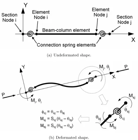
Starting from the connection modeling of springs with rotation stiffness, the presence of these last ones will introduce, as illustrated in Fig. 1, φci and φcj relative rotation values in i and j nodes of the member, respectively. Then, the equations that describe the nonlinear behavior of a structural system ideally rigid are modified. In Pinheiro [25], modifications were analyzed in two nonlinear formulations: that described by Torkamani et al. [34] and Yang and Kuo in its linearized form [37]. A simple way to obtain the stiffness matrix takes into account the final relationship of force-displacement of the beam-column member in the local coordinate system (see Fig. 2).

Among the several procedures used to modify the matricial equations of frame members for consideration of semi-rigid connections, three stand out: the methodologies described by Chan and Chui [6], Sekulovic and Salatic [31], and Chen and Lui [7]. All of them were also discussed and analyzed in Pinheiro [25]. Moreover, also in this last reference, the resulting matricial equations for the proposed procedures are detailed.

(a) Undeformated shape.

(b) Deformated shape.

Figure 1: Beam-column element with semi-rigid connections.

connection modeled in an analytical or mathematical way. Such procedures will be approached with more details in the following section, having also been treated in Pinheiro [25] and Pinheiro and Silveira [26].

3.1 Mathematical modeling of the semi-rigid connection

For a frame analysis with semi-rigid connections, the first procedure to be accomplished by a computational program is the reading of the parameters that characterize the behavior of each semi-rigid connection. Among the existent mathematical models used toward this end, there are the linear and nonlinear types. For a linear model, only one parameter defining the stiffness of a connection is required. The moment-rotation expression can be written as

Figure 2: Force-displacement relation used by Yang and Kuo [37] and its modification for con-sideration of semi-rigid connections.

where S_co is a constant value of the initial stiffness of a connection, which can be expressed in terms of the beam stiffness and of a rigidity index proposed to indicate the degree of joint flexibility. This index is the fixity factorγ of both nodes of the hybrid element. The fixity factor varies from zero, for the ideally pinned case, to 1, for the perfectly rigid case, and supplies the initial stiffness of the connection by expression

S_co = γ 1−γ

3EI

L , (2b)

In the case of a nonlinear model, usually a larger number of parameters are necessary. Such a model should be able to supply updated values of stiffness at each incremental-iterative step. A method commonly used to determine the moment-rotation relationship of connections is to fit a curve for experimental data using simple expressions. These expressions are called mathematical models, relating the moment and the rotation of the joints directly by mathematical functions, using some values of curve-fitting parameters. Since extensive tests in several types of connec-tions have been made in the last decades, much data, for various joint types, is accessible for obtaining the necessary parameters for the mathematical models. A good mathematical model should be simple, having physical meaning and requiring few parameters. Besides, it should always guarantee the generation of a smooth curve, with a positive first derivate, and to cover a wide range of connection types [6]. Among the several models that exist in the literature, three will be discussed here. The first of them is the exponential model, proposed by Lui and Chen [21, 22], whose mathematical expression of the moment-rotation curve is given by

M =Mo+ n X

j=1 Cj

·

1−exp µ

− |φc| 2jα

¶¸

+Rkf|φc|, (3a)

and its tangent connection stiffness has the form of

Sc= dM dφc ¯ ¯ ¯ ¯

|φc|=|φc|

= n X j=1 Cj 2jαexp µ − |φc|

2jα ¶

+Rkf, (3b)

in which M is the moment value in the connection, Mo the initial moment, | φc | the abso-lute value of the rotational deformation of the joint; Rkf the strain–hardening stiffness of the connection, α a scaling factor,n is the number of terms considered, andC_j is the curve-fitting coefficients.

In general, the Chen-Lui exponential model gives a good representation of nonlinear connec-tion behavior [6], in spite of requiring a large number of parameters for curve fitting. However, if there is an abrupt change in the moment-rotation curve sharp, this model could not represent it correctly. Consequently, Kishi and Chen [17, 18] modified the Chen-Lui model, so that this one could accomodate any accentuated change in M-φccurve. Under the loading condition, the function proposed by these researchers is written as

M =Mo+ m X

j=1 Cj

·

1−exp µ

− |φc| 2jα ¶¸ + n X k=1

D_k(|φc| − |φk|)H [|φc| − |φk|], (4a)

and its tangent connection stiffness has the form of

S_c= dM dφc ¯ ¯ ¯ ¯

|φc|=|φc|

= m X j=1 Cj 2jαexp µ − |φ_c|

2jα ¶ + n X k=1

where the values ofM,M_o,α, andC_j are the same as those defined by Eq. (3),φ_kis the starting rotations of linear components,Dk are curve-fitting constants for adjustment of the linear part of the curve, andH[φ] is the Heaviside step function defined as

H[φ] = 1 when φ≥0, (5a)

H[φ] = 0 when φ <0. (5b)

Among the several existing models for representation of semi-rigid connections behavior, one proposed by Richard-Abbott [28] describes the moment-rotation relationship as

M = (k−kp)|φc| h

1 +¯¯ ¯

(k−kp)|φc| Mo

¯ ¯ ¯

ni1/n +kp|φc|, (6a)

and the corresponding tangent stiffness by

S_c= dM dφc ¯ ¯ ¯ ¯

|φc|=|φc|

= (k−kp)

h 1 +

¯ ¯ ¯

(k−kp)|φc| Mo

¯ ¯ ¯

ni(n+1)/n +kp, (6b)

where k is the initial stiffness, kp is the strain-hardening stiffness, n is a parameter defin-ing the sharpness of the curve, and M₀ is a reference moment. Since this model needs only four parameters to characterize the joint behavior and always supplies a positive stiffness, it is an effective computational model, and one of the most used models to represent semi-rigid connections [6, 7, 30].

4 Computational procedures

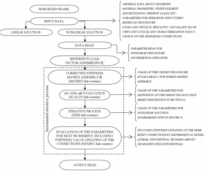
The general procedure for nonlinear solutions used in this work is illustrated in Fig. 3. After the reading of the general data of the structural system, accomplished in DATA 1, the next step is the reading of the second data file (DATA 2). In this last one is the information regarding the nonlinear solution strategy, such as the element nonlinear formulation to be used, the incre-ment and iteration strategies, the maximum number of iterations by increincre-ment, the convergence criterion, among other parameters relative to the chosen solution strategy. More details about the elaboration of this file can be found in the dissertations of Rocha [29] and Galv˜ao [14]. Following, some of the stages shown in Fig. 3 will be approached.

4.1 Initialization parameters

geometry, finite element discretization, conectivities between elements, material properties, etc. Additionally, this file also will have all of the necessary parameters for the characterization of the stiffness-rotation behavior of each semi-rigid connection inserted in the structure.

Figure 3: Flowchart of the general nonlinear solution.

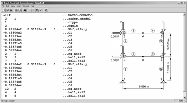
If a linear model to characterize a flexible joint has been used, only the information about which finite elements have semi-rigid nodes, which node is semi-rigid, and its respective fixity factor given by Eq. (2) are necessary. Fig. 4 illustrates the input data of a frame with four semi-rigid connections modeled by the Chen-Lui exponential function presented in the previous section. The pertinent data for this characterization are the following ones:

b) SRFOR: it indicates which modification procedure of the stiffness matrix to the flexible connections will be used. This variable can be 1, what takes to the sequence of Chen and Lui calculations [7]; 2, takes the Chan and Chui procedure [6]; or 3, signaling the use of the Sekulovic and Salatic calculations [31];

c) NMODEL: it indicates the number of models that will represent the nonlinearity of the semi-rigid connections used in the analysis. Since there are three options (exponential, modified exponential, and Richard-Abbott models), only one model can be chosen to represent the flexible connections of the structure, any associations two by two of those models, or even all of them. The last two cases can be useful in situations where not all of the existent connections in the structure can, or ought to, be represented by the same mathematical model, needing to use a certain model for a group of connections and another model, or even more than one, for another group(s). Then, NMODEL assumes values varying from 1 to 3. For the example in Fig. 4, since only the exponential model is used, NMODEL is equal to 1;

d) CTYPE: it indicates which model will be used for representation of the behavior of the connections, assuming a value of 1 for the use of the Chen-Lui exponential, 2 for the modified exponential, or 3 for the Richard-Abbott model. From now on, all of the following data are for the model chosen here. In the case of NMODEL to be equal to 2 or 3 (in other words, more than one mathematical model is being used to characterize the joints), after all the necessary data to this CTYPE were inserted, the new CTYPE value(s) should be entered and, since then, the corresponding data;

e) NGELM: it measures the number of hybrid element groups that have the same parameters strictly, in both nodes, to be used in the chosen model in CTYPE. In the example shown in Fig. 4, this value is 2, because there are only two groups of existent hybrid elements, although all the connections are represented by the same mathematical model: those with semi-rigid parameters only in the i node, and those with semi-rigid parameters only in the j node.

Figure 4: Input data example for a frame with single web angle joints.

and N should be inserted in order, to indicate the initial stiffness, the strain-hardening stiffness of the connection, the reference moment, and the parameter defining the sharpness of the curve, respectively. Soon afterwards, the finite elements that will receive these semi-rigid connections should be identified, what is made by the following data:

f) NG: represents the number of sub-groups of elements that have the same modeling pa-rameters;

g) NOSR: indicates which node has a stiffness variation. If NOSR is equal to 1, only the stiffness of i node will have nonlinear behavior, in other words, modeling by Eqs. (3), (4), or (6) for the connections located in the i node. If it is equal to 2, only the stiffness value of the connection located in the j node will be updated by the chosen model (modeling also by Eqs. (3), (4), or (6) for the connections located in the j node). Besides, if NOSR is equal to 3, both stiffnesses of the element nodes will be updated from the same model and parameters. However, if the connections of both nodes are represented by different mathematical models, or by the same model but with different parameters, first should be entered the first model and the data regarding the i node, with NOSR assuming a value of 41, and then, for the second model and for the same hybrid elements, entered the data regarding the j node, with NOSR equal to 42;

each one of NG sub-groups of elements described by the same modeling parameters.

4.2 Stiffness matrix assembling

For the stiffness matrix assembling of semi-rigid frames, three formulations can be chosen: Chan and Chui [6], Sekulovic and Salatic [31], and Chen and Lui [7]. Each one of these can act to modify the formulation originally described for frames with rigid connections described by Torkamaniet al.[34] or Yang and Kuo in its linearized form [37]. For each element, the following steps are executed:

1. Evaluation of the rotation matrix;

2. Evaluation of the stiffness matrix for each finite element. If the element have not flexible connections, the formation of the stiffness matrix will be made by the nonlinear formulation described in the second input data file, it can be chosen as proposed by [34] or [37]. Otherwise, if the element is rigid, the stiffness matrix will be calculated using the semi-rigid formulation selected in the first input data file by the SRFOR variable, presented in the subsection 4.1. Then, the methodology of [34] or [37] will be modified by the procedure proposed by [31], [7] or [6]. The descriptions of the respective matricial procedures are detailed in [25];

3. The stiffness matrix will be taken to the global system;

4. Finally, the element stiffness matrix will be stored in the global stiffness matrix of the structure.

4.3 Internal force vector assembling

In this stage of the nonlinear process, it is necessary to obtain the internal force vector for the hybrid element. The sequence of calculations to be accomplished for obtaining this vector is the following:

1. Obtaining the incremental natural displacements vector;

2. Calculation of the stiffness matrix of the hybrid element, followed by the steps 1 to 3 discussed in the procedure of the subsection 4.2;

3. Obtaining the incremental internal force vector by multiplication between the stiffness matrix of the hybrid element and the incremental natural displacement vector;

4. Identification of the internal forces that cause deformation in the element, in other words, nodal moments and axial force;

6. Transformation of the vector to the global system;

7. Finally, storage of the internal force vector of the element in the global internal force vector of the structure.

4.4 Iterative process

The initialization of the incremental-iterative process is accomplished by considering that the field of displacements and the structure tension state are already known for the last load step t, from where it wishes to determine the equilibrium configuration for the load step t+ ∆t. Figure 5 illustrates, consequently, the basic steps for a nonlinear solution from an incremental-iterative process based on the Newton-Raphson method, using, in that case, an arch-length type constraint equation [29].

Figure 5: Basic steps for iterative solution based on Newton-Raphson method coupled with arc-length technique [29].

In this process, it is necessary to say that:

• k is referred as an iteration number counter;

• k = 0, defines the predict incremental solution;

• k = 1, 2, ... defines the Newton-Raphson iterative cycle;

• ∆λand ∆d_{characterize the load parameter and nodal displacement increments, measured}

in the last equilibrium configuration;

• δλ and δd _{are the load parameter and nodal displacements corrections obtained during}

the iterative process.

4.5 Updating of the flexible connection stiffness

In structures where the connection stiffness also has a nonlinear behavior, it becomes necessary, therefore, to update this value at each load step. Then, it is necessary to intercede in the sub-routine (NEXINC) that updates the parameters used in the nonlinear analysis for the next increment. The updating of the semi-rigid values of the hybrid element follows the next steps:

1. Identification of the semi-rigid elements to be updated;

2. Evaluation of the relative rotation increment obtained during the last load step by divi-sion of the nodal incremental moment by the connection stiffness value in the reference configuration t;

3. Calculation of the total relative rotation by sum of the incremental value with the accu-mulated until the reference configuration t;

4. Assembling of the equation that describes the connection nonlinear behavior using a matrix that stores the data of the chosen model in CTYPE;

5. Obtaining the updated connection stiffness value by substitution of the total relative ro-tation in the expression obtained in the previous step.

Then, the new connection stiffness value from step 5 is used in the assembling of the stiffness matrix and internal force vector in the next load step. Besides, the accumulated relative rotation is updated to be used again in the following load step, where the procedures from 1 to 5 will be repeated after the convergence of the iterative process. More details about the necessary computational implementations for the analysis of frames with semi-rigid connections are in Pinheiro [25] and Pinheiro and Silveira [26].

5 Numerical examples

5.1 Nonlinear analysis of frames with floor variation

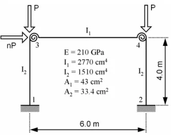
will be analyzed and compared: ideal connections (rigid and pinned) and semi-rigid. For this last one, two types of connections were considered, namely, double web angle (DWA) and top and seat double web angle (TSDWA). The data regarding these two connections were obtained from Sekulovic and Salatic [31] and Chen and Kishi [10] works.

The characteristic values for the horizontal displacement on the top of this frame regarding the first and second order analyses, both achieved for ideal and semi-rigid connections, are in Table 1. In addition, the bending moment values in the base of the structural system for linear and nonlinear analyses, as well as the critical loads, achieved following the semi-rigid element formulation proposed by Chan and Chui [6], are in Table 2.

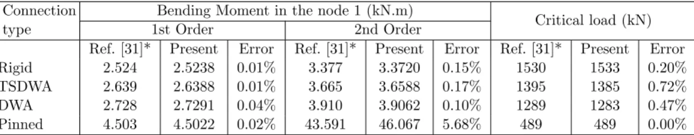
Figures 7 and 8 show the horizontal displacement on node 3 and the bending moment in node 1 as a function of the fixity factors between beam and column for different load levels. The division of these values with those obtained from the same frame with pinned connections normalizes the results.

Figure 6: Simple portal frame.

A variation of this example is presented in Fig. 9, in which a two-storey frame is shown. The dimensions of this structural system are in the same illustration, as well as the properties of their members. Tables 3 and 4 exhibit the results of linear and nonlinear analyses, both obtained for the ideal (rigid and pinned) and semi-rigid cases, using the same types of connections for simple portal frame.

The two tables previously mentioned show the difference among the results achieved for first and second order solutions. It can also be observed that the methodology of Chan and Chui [6] used in the nonlinear analysis produced, for most of the examined cases, similar results to those supplied by Sekulovic and Salatic [31].

Table 1: Horizontal displacements of node 3 in the simple portal frame, obtained using first and second order analyses (P = 450 kN, H = 0,005P).

Connection type

Horizontal displacement in the node 3 (×10−4m)

1st Order 2nd Order

Ref. [31]* Present Error Ref. [31]* Present Error

Rigid 25.79 25.788 0.01% 36.38 36.335 0.12%

TSDWA 28.70 28.693 0.02% 42.34 42.298 0.10%

DWA 30.95 30.971 0.07% 47.41 47.440 0.06%

Pinned 75.73 75.723 0.01% 868.69 923.792 6.34%

* Theoretical results supplied by Sekulovic and Salatic [31].

Table 2: Bending moment values for node 1 in the simple portal frame, obtained by first and second order analyses (P = 450 kN, H = 0,005P).

Connection type

Bending Moment in the node 1 (kN.m)

Critical load (kN) 1st Order 2nd Order

Figure 7: Influence of the connection flexibility for horizontal displacement on node 3.

Figure 9: Two-storey frame.

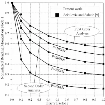
division of the critical load value for each one of the semi-rigid frames by that one achieved for ideally rigid connections case.

Table 3: Horizontal displacements of node 5 in the two-storey frame, obtained using first and second order analyses (P = 100 kN, H = 0,005P).

Connection type

Horizontal displacement in the node 5 (×10−4m)

1st Order 2nd Order

Ref. [31]* Present Error Ref. [31]* Present Error

Rigid 23.35 23.258 0.39% 25.45 25.429 0.08%

TSDWA 27.85 27.867 0.06% 31.10 31.101 0.00%

DWA 31.51 31.575 0.21% 35.78 35.834 0.15%

Pinned 176.61 176.609 0.00% 925.41 946.002 2.23%

Table 4: Bending moment values for node 1 in the two-storey frame, obtained by first and second order analyses (P = 100 kN, H = 0,005P).

Connection type

Bending Moment in the node 1 (kN.m)

Critical load (kN) 1st Order 2nd Order

Ref. [31]* Present Error Ref. [31]* Present Error Ref. [31]* Present Error Rigid 1.171 1.1709 0.01% 1.248 1.2468 0.10% 1115 1115 0.00% TSDWA 1.239 1.2392 0.02% 1.335 1.3346 0.03% 921 921 0.00% DWA 1.292 1.2923 0.02% 1.405 1.4051 0.01% 806 804 0.25% Pinned 3.001 3.0007 0.01% 12.457 12.4600 0.02% 122 122 0.00% * Theoretical results supplied by Sekulovic and Salatic [31].

5.2 Non-linear behavior of portal frames with semi-rigid connections

Now, the structure to be analyzed is a simple bay two-storey frame with nonlinear connections and different support conditions. Figure 11 shows the three situations considered for the sup-ports. For the case (b), an elastic support modeled by a spring with linear behavior, whose stiffness constant value is 0.1(EI/L)c, where the subscript “c” refers to the column. The value corresponds to, in the discretization carried out, a fixity factor equal to 0.032258064. The beams are wide flange shaped section W14×48 and were modeled with two finite elements, while the columns are wide flange shaped section W12×96 and were modeled by one element in the struc-tural model. Just like in the previous example, small lateral forces were applied to the frame to induce an imperfection to the structure. The magnitudes of those lateral forces are 0.001P on the top of the second floor and 0.002P on the top of the first floor.

Figure 11: Simple bay two-storey frame with different support conditions: (a) pinned; (b) semi-rigid; (c) fixed.

In these graphs the values of the present work were obtained from the computational imple-mentation accomplished using the semi-rigid element formulation proposed by [6]. Therefore, such values were compared with those supplied by these authors, with the exception done to the example in Fig. 11b, whose results are in Chen and Lui [21] (Fig. 14).

Figure 12: Moment-rotation curves represented by the Chen-Lui exponential model for the tested connections.

Figure 14: Load-deflection curves for semi-rigid support.

5.3 Six-Storey Frame (Vogel Frame)

The two bay six-storey frame with rigid connections shown in Fig. 16 was proposed by Vogel [35] as a calibration example to verify the accuracy of analyses and formulations of frames. Here, the structure will be used to compare results obtained among rigid and semi-rigid connection considerations in a nonlinear solution, while still having to investigate the constant and variable semi-rigid situations.

The total height of the frame is of 22.5 m and its total width is 12 m. The sections used for the members are presented in Fig. 16a and their properties are in Tab. 5. The uniformly distributed load was modeled as a group of equivalent nodal loads, as shown in Fig. 16b. Four finite elements were used to model each beam and one element was used for each column. Fig. 16b displays this discretization, including the numbering of the nodes and the equivalent nodal loads.

For the nonlinear solution, three situations were considered for the connections: ideally rigid, linear stiffness, and nonlinear stiffness. In order to obtain a more realistic behavior of the frame, the four types of connections used are presented in Fig. 12. In this analysis, as in the previous example, the Chen-Lui exponential model was used for the moment-rotation behavior, whose parameters used in the mathematical expression is described in Chan and Chui [6] and Pinheiro [25]. For the hypothesis of the connection to have a linear behavior, only the initial value of stiffness, also achieved in the Chen-Lui model, is taken into account.

Table 5: Geometrical properties of the steel sections used in the Vogel frame.

Perfil d b tw tf k A Ix Iy Zx

(mm) (mm) (mm) (mm) (mm) (cm2) (cm4) (cm4) (cm3)

IPE240 240 120 6.2 9.8 15 39.1 3892 284 367

IPE300 300 150 7.1 9.8 15 53.8 8356 604 628

IPE330 330 160 7.5 10.7 18 62.6 11770 788 804

IPE360 360 170 8.0 11.5 18 72.7 16270 1043 1019

IPE400 400 180 8.6 12.7 21 84.5 23130 1318 1307

HEB160 160 160 8.0 13.5 15 54.3 2492 889 354

HEB200 200 200 9.0 15.0 18 78.1 5692 2003 643

HEB220 220 220 9.5 16.0 18 91.0 8091 2843 827

HEB240 240 240 10.0 17.0 21 106.0 11260 3923 1053

HEB260 260 260 10.0 17.5 24 118.0 14920 5135 1283

are the equilibrium paths for the same structure, but with considerations for the connection stiffness varying nonlinearly according to the exponential model. For a better comparison of the results, Fig. 18 exhibits all the paths found by the accomplished computational implementation, considering the four initial assumptions of the connection stiffness.

(a) (b)

Figure 17: Vogel frame analysis: (a) linear connections; (b) nonlinear connections.

6 Conclusions and comments

This article had a main objective: to illustrate some of the computational details necessary for the nonlinear analysis of steel structured frames with semi-rigid connections. Computational aspects related to a strategy of incremental-iterative solution, connection stiffness and moment-rotation curves were discussed.

Figure 18: Comparison between the various joint types for the Vogel frame.

of the connection, supplying a new stiffness, was decisive for the obtaining of the accuracy demonstrated in the results.

Additionally, it can be concluded that the nonlinear formulation proposed by Yang and Kuo [37] for frames without flexible joints can be adapted and adjusted perfectly when the presence of them, producing identical results to those presented by Chan and Chui [6]. This methodology, likewise, demonstrates an equivalency to that proposed by Sekulovic and Salatic [31], as the results obtained for the first example of the section 5 demonstrate.

In the examples provided, it is clear from the final results that there is a significant difference between the results obtained from frames with ideal connections and those with semi-rigid connections. Besides, the influence of the second order theory can be seen, in the first example, by difference between the results obtained for linear and nonlinear analyses. It is necessary to point out that in those analyses the stiffness values of the connections DWA and TSDWA were worked in terms of the fixity factor values, which were given by Sekulovic and Salatic [31].

Acknowledgements: The authors acknowledge the support of the USIMINAS, FAPEMIG and National Council for Scientific and Technological Development (CNPq) for this work.

References

[1] Eurocode 3.Eurocode 3 Design of Steel Structures: Part 1.1, General Rules and Rules for Buildings, DD ENV 1993-1-1. 1992.

[2] K.M. Abdalla and W.F. Chen. Expanded database of semi-rigid steel connections. Comp. Struct., 56(4):553–564, 1995.

[3] K.M. Ang and G.A. Morris. Analysis of three-dimensional frames with flexible beam-column con-nections. Can. J. Civil Eng., 11:245–254, 1984.

[4] Standards Australia. AS-4100: Australian Standard for Steel Structures. Sydney, 1998.

[5] A. Azizinamini, J. H. Bradburn, and J. B. Radziminski.Static and cyclic behavior of semi-rigid steel beam-column connections, Technical Report. Dept. of Civil Engineering, Univ. of South Carolina, Columbia, SC, 1985.

[6] S. L. Chan and P. P. T. Chui.Nonlinear Static and Cyclic Analysis of Steel Frames with Semi-Rigid Connections. Elsevier, Oxford, 2000.

[7] W. F. Chen and W. M. Lui. Stability Design of Steel Frames. CRC Press, Boca Raton, Fl´orida, 1991.

[8] W. F. Chen and I. Sohal.Plastic Design and Second-order Analysis of Steel Frames. Springer-Verlag, New York, 1995.

[9] W. F. Chen and S. Toma. Advanced Analysis of Steel Frames. CRC Press, Boca Raton, Fl´orida, 1994.

[10] W.F. Chen and N. Kishi. Semi-rigid steel beam-to-column connections: Data base and modeling.

J. Struct. Div. ASCE, 115(1):105–119, 1989.

[11] P. P. T. Chui and S. L. Chan. Vibration and deflection characteristics of semi-rigid jointed frames.

Engineering Structures, 19(12):1001–1010, 1997.

[12] M. J. Clarke and M. J. Hancock. A study of incremental-iterative strategies for non-linear analyses.

Int. J. Numer. Methods Eng., 29:1365–1391, 1990.

[13] M.J. Frye and G.A. Morris. Analysis of flexibly connected steel frames.Can. J. Civil Eng., 2(3):280– 291, 1975.

[14] A. S. Galv˜ao.Nonlinear Finite Element Formulations for Slender Structural Elements. M.Sc. Thesis. PROPEC/Deciv/School of Mines, UFOP (in Portuguese), 2000.

[15] N. D. Johnson and W. R. Walpole. Bolted end-plate beam-to-column connections under earthquake type loading, Research report 81-7. Dept. of Civil Engineering, Univ. of Canterbury, Christchurch, New Zealand, 1981.

[17] N. Kishi and W. F. Chen.Data Base of Steel Beam-to-Column Connections. Structural Engineering Report No. CE-STR-93-15. School of Civil Engineering, Purdue Univ., West Lafayette, IN, 1986.

[18] N. Kishi and W. F. Chen.Steel Connection Data Bank Program. Structural Engineering Report No. CE-STR-86-18. School of Civil Engineering, Purdue Univ., West Lafayette, IN, 1986.

[19] T. S. Kruger, B. W. J. van Rensburg, and G. M. du Plessis. Nonlinear analysis of structural steel frames. J. Construct. Steel Research, 34:285–306, 1995.

[20] L. R. O. Lima, S.A.L. Andrade, P.C.G. Vellasco, and L.S. Silva. Experimental and mechanical model for predicting the behaviour of minor axis beam-to-column semi-rigid joints. Int. J. Mech. Sciences, 44:1047–1065, 2002.

[21] E. M. Lui and W. F. Chen. Behavior of braced and unbraced semi-rigid frames. International Journal of Solids Structures, 24(9):893–913, 1988.

[22] E.M. Lui and W. F. Chen. Analysis and behavior of flexibly jointed frames.Engineering Structures, 8:107–118, 1986.

[23] American Institute of Steel Construction. LRFD Load and Resistance Factor Design Specification for Structural Steel Buildings. AISC, Chicago, 2000.

[24] J. R. Ostrander. An experimental investigation of end-plate connections, Masters thesis. Univ. of Saskatchewan, Saskatoon, SK, Canada, 1970.

[25] L. Pinheiro. Non-Linear Analysis of Spatial Truss and Plane Frames with Semi-Rigid Connections, M.Sc. Thesis. PROPEC/Deciv/School of Mines, UFOP (in Portuguese), 2003.

[26] L. Pinheiro and R. A. M. Silveira. Nonlinear analysis of steel frames with semi-rigid connections. In

Proceedings of the XXIV Iberian-Latin American Congress of Computational Methods in Engineering (XXIV CILAMCE), volume 1, pages 1–18, Ouro Preto/Brazil, 2003. (CD-ROM) (in Portuguese).

[27] R. M. Richard, J. D. Kreigh, and D. E. Hornby. Design of single plate framing connections with a307 bolts. Eng. J. AISC, 19(4):209–213, 1982.

[28] R.M. Richard and B.J. Abbott. Versatile elastic-plastic stress-strain formula.Journal of Engineering Mechanics, Div. ASCE, 101(4):511–515, 1975.

[29] G. Rocha. Load Increment and Iterative Strategies for Nonlinear Analysis of Slender Structural Systems. M.Sc. Thesis. PROPEC/Deciv/School of Mines, UFOP (in Portuguese), 2000.

[30] M. Sekulovic and M. Nefovska-Danilovic. Static inelastic analysis of steel frames with flexible con-nections. Theoret. Appl. Mech., 31(2):101–134‘, 2004.

[31] M. Sekulovic and R. Salatic. Nonlinear analysis of frames with flexible connections. Computers and Structures, 79(11):1097–1107, 2001.

[32] R. A. M. Silveira. Analysis of Slender Structural Elements under Unilateral Contact Constraints. Ph.D. Thesis. Civil Engineering Department, Pontifical Catholic University of Rio de Janeiro (PUC-Rio), Rio de Janeiro/RJ/Brazil, 1995. 211 p (in Portuguese).

[34] M. A. M. Torkamani, M. Sonmez, and J. Cao. Second-order elastic plane-frame analysis using finite-element method. Journal of Structural Engineering, 12(9):1225–1235, 1997.

[35] U. Vogel. Calibrating frames. Stahlbau, 54:295–311, 1985.

[36] L. Xu. Second-order analysis for semi-rigid steel frame design. Canadian Journal of Civil Engineer-ing, 28:59–76, 2001.

[37] Y. B. Yang and S. R. Kuo. Theory & Analysis of Nonlinear Framed Structures. Prentice Hall, 1994.