A Bayesian view of the Higgs sector with higher dimensional operators

(1)

JHEP07(2013)065

Published for SISSA by Springer

Received_: April 29, 2013 Revised: June 7, 2013 Accepted: June 17, 2013 Published: July 10, 2013

A Bayesian view of the Higgs sector with higher

dimensional operators

Beranger Dumont,a Sylvain Fichetb and Gero von Gersdorffc,d

a_{Laboratoire de Physique Subatomique et de Cosmologie, UJF Grenoble 1, CNRS/IN2P3, INPG,}

53 Avenue des Martyrs, F-38026 Grenoble, France b_{International Institute of Physics, UFRN,}

Av. Odilon Gomes de Lima, 1722 - Capim Macio - 59078-400 - Natal-RN, Brazil c_{Centre de Physique Th´eorique, ´}_{Ecole Polytechnique and CNRS,}

F-91128 Palaiseau, France

d_{ICTP South American Institute for Fundamental Research,}

Instituto de Fisica Teorica, Sao Paulo State University, Sao Paulo, SP 01140-070, Brazil

E-mail: dumont@lpsc.in2p3.fr,sylvain.fichet@lpsc.in2p3.fr,

gersdorff@gmail.com

Abstract: _{We investigate the possibilities of New Physics affecting the Standard Model}

(SM) Higgs sector. An effective Lagrangian with dimension-six operators is used to capture the effect of New Physics. We carry out a global Bayesian inference analysis, considering the recent LHC data set including all available correlations, as well as results from Tevatron. Trilinear gauge boson couplings and electroweak precision observables are also taken into account. The case of weak bosons tensorial couplings is closely examined and NLO QCD corrections are taken into account in the deviations we predict. We consider two scenarios, one where the coefficients of all the dimension-six operators are essentially unconstrained, and one where a certain subset is loop suppressed. In both scenarios, we find that large deviations from some of the SM Higgs couplings can still be present, assuming New Physics arising at 3 TeV. In particular, we find that a significantly reduced coupling of the Higgs to the top quark is possible and slightly favored by searches on Higgs production in association with top quark pairs. The total width of the Higgs boson is only weakly constrained and can vary between 0.7 and 2.7 times the Standard Model value within 95% Bayesian credible interval (BCI). We also observe sizeable effects induced by New Physics contributions to tensorial couplings. In particular, the Higgs boson decay width into Zγ can be enhanced by up to a factor 12 within 95% BCI.

Keywords: _{Higgs Physics, Beyond Standard Model}

(2)

JHEP07(2013)065

Contents

1 Introduction 1

2 Electroweak higher-dimension operators 3

2.1 Effective Lagrangian 5

2.2 Standard Model loop-induced HDOs 7

2.3 Trilinear gauge boson vertices 7

3 Data treatment 8

4 On weak bosons tensorial couplings 10

4.1 h_→V V∗ ₁₂

4.2 VBF production mode 13

4.3 VH production mode 14

5 Deviations caused by New Physics 14

5.1 Higgs signal strengths 14

5.2 QCD radiative corrections 16

5.3 S andT parameters 16

6 Bayesian setup and low-Λ scenario 17

6.1 Bayesian inference 17

6.2 Priors and low-Λ scenarios 18

6.3 The MCMC setup 20

7 Inference on HDOs 20

8 Conclusion 28

A Deriving the tree-level effective Lagrangian 30

B Loop-induced SM couplings 31

C Tensorial Higgs decay to weak bosons 32

1 Introduction

(3)

JHEP07(2013)065

the excess around 125 GeV reaches more than 7 σ in both experiments. The analyses are based on up to 5 fb−1 _{at 7 TeV and 21 fb}−1 _{at 8 TeV, collected in 2011 and 2012.}

Following this fundamental breakthrough, new questions need to be addressed. Some of them may find an answer during the LHC era, through the analysis of the properties of the new boson. A first question is whether or not this resonance is a Higgs boson, i.e. the manifestation of a field involved in the electroweak symmetry breaking (EWSB) and unitarization ofW W scattering. Second, if it is indeed a Higgs, one may wonder to what extent it is compatible with the Standard Model Higgs. Indeed, the properties of the Higgs boson could be dramatically modified with the theoretical prejudice that New Physics has to emerge near the electroweak scale. On the other hand, direct searches for new states beyond the SM have so far turned out to be unsuccessful, and indirect constraints from electroweak precision measurements at LEP push the limits on masses of new particles somewhat further above the electroweak scale. If New Physics is indeed present and is somehow separated from the electroweak scale, the couplings of the Higgs boson will be close to those of the SM and will only be modified by the effect of a few higher dimensional operators. In this paper, we will explore an effective field theory (EFT) with only relatively few new parameters.

Many aspects of these fundamental questions have already been investigated in several works (see e.g. [3–14] for studies based on the 8 TeV results). For example, the chiral EW Lagrangian with a non-linear realization of the SU(2)L×U(1)Y symmetry is a quite gen-eral framework in order to study the properties of electroweak symmetry breaking. Many scenarios producing possibly large deviations with respect to the SM Higgs properties are successfully captured in such EFT approach.

We are going to consider that new states appear at a typical scale Λ substantially larger than the electroweak scale. For physical processes involving an energy scale smaller than Λ, New Physics can be integrated out. As a consequence of this hypothesis, the resulting low-energy effective theory consists in the Standard Model, supplemented by infinite series of local operators with higher dimension, which involves negative powers of Λ,

Leff =LSM+

X

i

αi

ΛniOi. (1.1)

The effects of such higher dimensional operators (HDOs) have been investigated in many contexts such as flavor physics, or the study of the properties of the electroweak gauge bosons through LEP precision measurements. The purpose of this paper is to study the electroweak sector again, which now includes new Higgs observables. For our analysis, we only have to consider the leading HDOs. The only operator with ni = 1 is the one giving a Majorana mass to the neutrino, and is not relevant for our study. We will thus be exclusively interested in the n= 2 terms, i.e. dimension-6 operators.

(4)

JHEP07(2013)065

considered as generic, i.e. free of improbable cancellations. Our Bayesian analysis will rely on Markov chain Monte Carlo (MCMC) techniques, which allows us to easily sample the posterior probability distribution function.

The outline of the paper is as follows. In section2, we lay out the formalism for higher-dimension operators in the electroweak sector. In section3, we present the dataset used for the analysis and the measurements entering the likelihood functions. The peculiar case of observables sensitive to tensorial couplings relating Higgs and weak bosons is investigated in section 4. In section 5, we derive the observable deviations from the SM induced by the higher dimensional operators, taking into account leading NLO QCD effects. Section6

presents the setup of our Bayesian analysis. Section 7 is devoted to our results. Our conclusion is given in section8.

2 Electroweak higher-dimension operators

In this section, we define the basis of dimension-6 operators supplementing the renormal-izable electroweak sector of the SM Lagrangian. We refer to [17,18] for further details on the Standard Model HDOs.

A basis of CP-even operators not involving fermions can be chosen as1

O6 =|H|6, OD2 =|H|2|D_µH|2, O′_D2 =|H†DµH|2, (2.1) OWW =H†H(Wµνa )2, OBB =H†H(Bµν)2, OWB =H†WµνH Bµν, (2.2)

OGG=H†H(Gaµν)2. (2.3)

Any other operator can be reduced to these via integration by parts and the use of the SM equations of motion for the Higgs and gauge fields, possibly generating operators involving fermions. Amongst the latter, only a limited set will be relevant for our purpose. Operators of the form JH ·Jf, where JH and Jf are SU(2) or U(1)Y currents involving Higgs field and fermionf respectively, will in general contribute to FCNC as well as electroweak non-oblique corrections (e.g., non-universal couplings of fermions to gauge bosons).2 _However,

the operators

OD =JH µa Jµa, OD′ =JH µY JµY , (2.4) whereJ =P

fJf are the SM fermion currents coupling toBµand Wµ, are flavor diagonal and only result in universal corrections to gauge couplings and should hence be viewed as contributing toS andT.3 We will also need to consider Yukawa corrections of the form

Of = 2yf|H|2Hf¯LfR, (2.5)

1_{The operator}_O

6 plays no role in what follows and is listed here only for completeness.

2_{The non-universal corrections to the weak bosons couplings of the top quark are only very mildly}

constrained by EW data, and it is a priori not justified to set them to zero. However the only effect to Higgs observables at leading order is a modification of the top loop contribution to the h → Zγ decay due to the anomalousZtt vertex. The top contribution is however about one order of magnitude smaller than the leading contribution from theW loop [19]. We will therefore only consider universal (oblique) corrections to EW data.

3_{In fact this is the way how contributions to}_S _and_T _{can arise in theories with new spin-1 states, such}

(5)

JHEP07(2013)065

where fR=tR, bR, τR and fL the corresponding doublet ( ¯f_La =ǫabq¯b,3_L , q¯_La,3,ℓ¯a,3_L ) and yf the Yukawa coupling.

Note that the operators _OD and O′D could be traded for the operators

OW = (DµH)†WµνDνH , OB = (DµH)†DνH Bµν, (2.6)

by use of the SM equations of motion for B and W. While _OD and OD′ contribute to S andT but not to the modified Higgs couplings, for_OB andOW it is the other way around. Both choices of basis are physically equivalent. Before passing from a general redundant set of operators to a convenient irreducible basis via the equations of motion, it is useful to first identify the operators that cannot be generated at tree-level. This is valuable in-formation and we would like to avoid it to be lost in the course of the reduction. However this is what would happen if we eliminated _OD and O′_D in favor of OW and OB. Indeed, this would cause the coefficient of e.g. _OWB (which cannot be generated at tree-level) to be shifted by the coefficient of_OD (which can be generated at the tree-level via exchange of spin-one states). This is why we choose this basis.

The only remaining two-fermion operators are of the dipole type. These operators are tightly constrained by FCNC as well as by their contributions to electric and magnetic dipole moments. Moreover, they are necessarily generated at the loop-level, and only affect Higgs couplings to gauge bosons by modifying existing SM loops. They will not have any impact on our results, therefore we can neglect them entierely.

We do not take into account CP-violating HDOs. These operators are constrained by observables such as electric dipole moments. If we choosed to include these CP-odd HDOs in our analysis, we would also need to consider the whole set of data sensitive to CP violation. Although there is no fundamental problem with such extended analysis, that is beyond the scope of the present work. Moreover, the effects induced by CP-violating HDOs are often subleading with respect to the effects of CP-even operators, unless the latter are sufficiently suppressed. This is the case for Higgs decays, because CP-violating amplitudes do not interfere with SM amplitudes, whereas CP-conserving amplitudes do interfere with SM amplitudes [22]. In the following we will derive observable deviations from the Standard Model using the full set of HDOs, and perform the analysis presented in section 6taking into account only operators that respect custodial symmetry.

(6)

JHEP07(2013)065

2.1 Effective Lagrangian

In this section we will present the effect of the HDOs on the SM tree-level couplings. Loops involving SM particles are considered in section2.2. We define the physical Higgs fieldhas

H=





0 1 √

2(˜v+h)



 , (2.7)

and parametrize the couplings of h to gauge bosons and fermions as4

Ltreev,f =λZh(Zµ)2+λWh Wµ+Wµ−+

X

f

λfhf¯LfR. (2.8)

The SM tree-level predictions for these quantities are given in terms of the SM input parameters ˜g, ˜v and ˜s2_w_≡g˜′2/(˜g2+ ˜g′2):

λZ = ˜

g2_v_˜ 4 ˜c2

w ≡ ˜

m2_Z

˜

v , λW =

˜

g2_v_˜

2 ≡

2 ˜m2_W

˜

v , λf =−

˜

yf √

2 ≡ − ˜

mf ˜

v , (2.9)

where the quantities with a tilde are the ones that appear in the SM part of the Lagrangian. For instance, ˜g and ˜g′ _{are the couplings appearing in the covariant derivatives. However,} these couplings do not take the same values as in the SM, since there are corrections from HDOs. There are distinct effects, as follows (see ref. [25] for an analogous discussion on fermion couplings).

• Operators such as_O_D2 correct directly the tree-level SM vertices.

• Some operators (e.g._O_D2,O_WW) modify the kinetic terms of Higgs and gauge fields

and thus indirectly lead to the rescaling of some couplings.

• Finally, there can be indirect effects from input parameters. They are taken to be the fine-structure constantα, theZboson massmZ and the Fermi constantGF, as well as the physical fermion massesmf and the strong coupling constantαs. These quantities receive corrections from HDOs but must be held fixed in the analysis. Yet, this causes the SM parameters ˜g, ˜v and ˜sw to become functions of the HDO coefficients.

The last point is sometimes not taken into account in the literature. Let us focus on it anddefine the quantitiesv,g and sw via

4πα_≡s2_wg2, m2_Z_≡ v

2_g2

4c2 w

, GF ≡ 1 √

2v2 . (2.10)

These quantities can be viewed as the “familiar” numbers from the SM (e.g.v= 246 GeV). Like the input parameters they stay fixed in our analysis. On the other hand, the param-eters ˜g, ˜sw and ˜v are the gauge couplings appearing in the covariant derivatives and the vacuum expectation value (vev) of the Higgs field, and must be expressed in terms of the

(7)

JHEP07(2013)065

HDO coefficients. We present the details of this procedure in appendix A. Taking into account all the above effects, we obtain

λZ =aZ

m2 Z

v , λW =aW

2m2 W

v , λf =−cf mf

v , (2.11)

wheremf and mW are the physical masses. In particular, mW is given by5

m2_W = g 2_v2

4

1 +

1 2αD−

c2_w

2(c2 w−s2w)

[α′_D2+αD]−

cwsw

c2 w−s2w

αWB v2 Λ2 = g 2_v2

4

1₋ αS

2(c2 w−s2w)

+ c 2 wαT

c2 w−s2w

. (2.12)

In the last row we have used eqs. (5.13) and (5.14) in order to compare our derivation of

mW with the one in [25]. The SM prediction ofmW is thus only corrected by the oblique parameters. In this parametrization, the rescaling factorsaZ,aW andcf are given by

aZ = 1 +

1 2αD2 −

1 4αD +

1 4α ′ D2 v2

Λ2 ,

aW = 1 +

1 2αD2 −

1 4αD −

1 4α ′ D2 v2 Λ2 ,

cf = 1−

1 4α

′ D2 −

1

4αD −αf

v2

Λ2. (2.13)

As a nontrivial consistency check, note that the vector anomalous couplings are rescaled in a custodially symmetric way (aZ = aW) once the custodial-symmetry violating operator

O′

D2 is turned off.

To conclude this subsection we compute the direct tree-level HDO contribution to the tensor couplings,

Ltreet =ζγh(Fµν)2+ζgh(Gµν)2+ζZγh FµνZµν +ζZh(Zµν)2+ζWh Wµν+Wµν− , (2.14)

which are all zero in the SM at tree-level. One finds

ζγ =

s2_wαWW +c2wαBB− 1

2swcwαWB

v

Λ2 , ζg=αGG

v

Λ2, (2.15)

ζZγ =

2cwswαWW −2cwswαBB− 1 2(c

2

w−s2w)αWB

v

Λ2, (2.16)

ζZ =

c2_wαWW +s2wαBB+ 1

2cwswαWB

v

Λ2 , ζW = 2αWW

v

Λ2 . (2.17)

The first two quantities constitute important corrections to the production and decay of the Higgs boson. The last two corrections modify the tensorial structure of the SM Higgs-weak bosons coupling in a non-trivial way, which is discussed in detail in section4.

5_Unlike_m

Zandmf, which are input parameters, theWmass is a prediction in terms of input parameters

(8)

JHEP07(2013)065

2.2 Standard Model loop-induced HDOs

In this section we compute the Standard Model loop-induced operators relevant for Higgs physics. These operators contain indirect modifications due to couplings modified by the HDOs considered in the previous subsection. We want to make sure that we do not double-count possible New Physics contribution to the Higgs couplings. In order to have a well-defined HDO framework at loop-level, we should consider that the HDOs we present in eqs. (2.1)–(2.5) are generated exclusively through New Physics states at leading order, and enclose higher-order SM corrections only from irreducible loops.6 _{Hence, the modified SM}

loops are not included in the tree-level contributions computed in the previous subsection. Our strategy is thus to compute the one-loop corrections to_Ltreeusing the couplings shown in eq. (2.13).

The one-loop Lagrangian is parametrized as

L1−loop=λγh(Fµν)2+λgh(Gµν)2+λZγh FµνZµν. (2.18)

Let us decompose these couplings according to the particle in the loop, λi =P_XλX_i . We find7

λW_γ =aWλW,SMγ = 7 2

g2_s2 w 16π2

aW

v Av(τW), (2.19)

λf_γ =cfλf,SMγ =− 2 3N

c fe2f

g2_s2 w 16π2

cf

v Af(τf), λ

f

g=cfλf,SMg =− 1 3

g2 s 16π2

cf

v Af(τf), (2.20)

λW_Zγ =aWλW,SM_Zγ =

e2

16π2

aW v t −1 w 2

t2_w₋3

AZγ(τW, κW)

+

5₋t2 w

2 +

1₋t2 w

τW

BZγ(τW, κW)

, (2.21)

λf_Zγ =₋cfλf,SMZγ =

e2

16π2

cf

v N

c f

e2_f(T_f3L₋2efs2w)

swcw

BZγ(τf, κf)−AZγ(τf, κf)

. (2.22)

whereNc

f andef are the number of colors and the fraction of electric charge of the fermion running in the loop, respectively. We define τi = 4m2i/m2h, κi = 4m2i/m2Z . The form factors Ai, B are given in appendix B. They are defined so that in the decoupling limit,

Af,v →1 when τ → ∞, andAZγ →1,BZγ →0 whenτ, κ→ ∞.

2.3 Trilinear gauge boson vertices

The higher dimensional operators that we are considering also affect charged triple gauge boson vertices (TGV). In the parametrization of ref. [26],

LTGV=−i e κγFµνWµ−Wν+−i g cwκZZµνWµ−Wν+−i g cwg1Z

W_µν+W−

ν −Wµν−Wν+

Zµ, (2.23)

6_{This last point is important for NLO QCD corrections, see section}₅_.

7_{Note that in eqs. (}_2.19_)–(_2.22_{) only the quantites with a tilde appear. Besides the modified Higgs}

(9)

JHEP07(2013)065

the deviations from the Standard Model can be expressed in terms of the HDO coefficients as follows:

κγ = 1 +

αWB 2tw

v2

Λ2 ,

κZ = 1−

swcw (c2

w−s2w)

αWB+ 1 4(c2

w−s2w) [α′

D2 +αD]

v2 Λ2,

gZ₁ = 1₋

sw 2cw(c2w−s2w)

αWB+ 1 4(c2

w−s2w)

[α′_D2+αD]

v2

Λ2 , (2.24)

where again some indirect effects from fixing input parameters were taken into account. Gauge invariance implies the relation κZ =g1Z−(κγ −1)t2w and one can check that it is indeed fulfilled. We then chooseκγ and gZ1 as independent couplings.

3 Data treatment

We exploit the results from Higgs searches at the LHC and at Tevatron as well as elec-troweak precision observables and trilinear gauge couplings. The results from Higgs searches are given in terms of signal strengths µ(X, Y), the ratio of the observed rate for some processX _→h_→Y relative to the prediction for the SM Higgs. An experimental channel is defined by its final state (γγ, ZZ, Zγ, W W, b¯b, τ τ) and is often divided into subchannels having different sensitivity to the various production processes. The accessible production mechanisms at the LHC arei)gluon-gluon fusion (ggF),ii)vector boson fusion (VBF), iii) associated production with an electroweak gauge boson V =W, Z (VH), and iv) associated production with at¯t pair (ttH).

As higher dimensional operators modify not only the Higgs decays but also its production (see section 5), care has to be taken in extracting the information given by the experiments. In particular, when available, we use the results given in the plane (µ(ggF + ttH, Y), µ(VBF + VH, Y)), which (partly) account for the correlations between the subchannels.

The values for the signal strengths in the various (sub)channels as reported by the experiments and used in this analysis, together with the estimated decompositions into production channels are given in tables 1–3. Some of the decompositions into production channels are taken from [27]. In case of missing information, we take the relative ratios of production cross sections for a SM Higgs as a reasonable approximation, i.e. we assume that the experimental search is fully inclusive and compute the signal strength modified by HDOs accordingly. To this end, we use the latest predictions of the cross sections at the LHC [28] and at Tevatron [29].

In both ATLAS and CMS, the Higgs mass is estimated from the two “high-resolution” channels: ZZandγγ. In our analysis, the Higgs mass is set tomh= 125.5 GeV (close to the combined mass measurement from the two experiments) since it is not yet possible the take it as a nuisance parameter without losing the correlations between production channels. We consider experimental measurements of the signal strengths as close as possibe to this value. We take into account the electroweak precision observables using the Peskin-Takeuchi

(10)

JHEP07(2013)065

Channel Signal strengthµ mh (GeV) Production mode

ggF VBF WH ZH ttH

h_→γγ (4.8 fb−1 _{at 7 TeV + 20.7 fb}−1 _{at 8 TeV) [}₃₀_,₃₁_]

µ(ggF + ttH, γγ) 1.60_±0.41 125.5 100% — — — —

µ(VBF + VH, γγ) 1.94_±0.82 125.5 — 60% 26% 14% —

h_→ZZ (4.6 fb−1 _{at 7 TeV + 20.7 fb}−1 _{at 8 TeV) [}₃₁_,₃₂_]

µ(ggF + ttH, ZZ) 1.51_±0.52 125.5 100% — — — —

µ(VBF + VH, ZZ) 1.99_±2.12 125.5 — 60% 26% 14% —

h_→W W (4.6 fb−1 _{at 7 TeV + 20.7 fb}−1 _{at 8 TeV) [}₃₃_,₃₄_]

µ(ggF + ttH, W W) 0.79_±0.35 125.5 100% — — — —

µ(VBF + VH, W W) 1.71_±0.76 125.5 — 60% 26% 14% —

h_→b¯b (4.7 fb−1 _{at 7 TeV + 13.0 fb}−1 _{at 8 TeV) [}₃₁_,₃₅_]

VH tag ₋0.39_±1.02 125.5 — — 64% 36% —

h_→τ τ (4.6 fb−1 at 7 TeV + 13.0 fb−1 at 8 TeV) [31]

µ(ggF + ttH, τ τ) 2.31_±1.61 125.5 100% — — — —

µ(VBF + VH, τ τ) ₋0.20_±1.06 125.5 — 60% 26% 14% —

Table 1. ATLAS results, as employed in this analysis. The following correlations are included in the fit: ργγ =−0.27,ρZZ =−0.50,ρWW =−0.18,ρτ τ =−0.49.

be used in the HDO framework. However we find that constraints arising from these parameters are by far subleading with respect to our other constraints. Experimental values of S and T are taken from the latest electroweak fit of the SM done by the Gfitter Group [51]: S = 0.05_±0.09 and T = 0.08_±0.07 with a correlation coefficient of 0.91. Regarding constraints on TGV, we take into account the LEP measurements [52]:

κγ = 0.973+0.044₋0.045,

g₁Z = 0.984+0.022₋_0.019. (3.1)

The global likelihood function is defined as the product of the likelihoods associated to the various observables,

L=LHiggs×LS,T ×LTGV, (3.2)

where LHiggs is the product of the likelihoods associated to each of the experimental (sub)categories, including available correlations. The likelihood associated to the mea-surement of an observable ˆO, given as a central value O and a symmetric uncertaintyσ, is modeled by a normal law,

LO∝e−(O− ˆ O)2_/2σ2

. (3.3)

(11)

JHEP07(2013)065

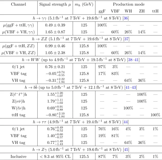
Channel Signal strength µ mh (GeV) Production mode

ggF VBF WH ZH ttH

h_→γγ (5.1 fb−1 _{at 7 TeV + 19.6 fb}−1 _{at 8 TeV) [}₃₆_]

µ(ggF + ttH, γγ) 0.49_±0.39 125 100% — — — —

µ(VBF + VH, γγ) 1.65_±0.87 125 — 60% 26% 14% —

h_→ZZ (5.1 fb−1 _{at 7 TeV + 19.6 fb}−1 _{at 8 TeV) [}₃₇_]

µ(ggF + ttH, ZZ) 0.99_±0.46 125.8 100% — — — —

µ(VBF + VH, ZZ) 1.05_±2.38 125.8 — 60% 26% 14% —

h_→W W (up to 4.9 fb−1 _{at 7 TeV + 19.5 fb}−1 _{at 8 TeV) [}₃₈_–₄₁_]

0/1 jet 0.76_±0.21 125 97% 3% — — —

VBF tag ₋0.05+0.74₋_0.55 125.8 17% 83% — — —

VH tag ₋0.31+2.22₋_1.94 125.8 — — 64% 36% —

h_→b¯b (up to 5.0 fb−1 at 7 TeV + 12.1 fb−1 at 8 TeV) [41–43]

Z(ℓ−_ℓ+_)h ₁_.₅₅+1.20

−1.07 125 — — — 100% —

Z(νν¯)h 1.79+1.11_−1.02 125 — — — 100% —

W(ℓν)h 0.69+0.91_−0.88 125 — — 100% — —

ttH tag ₋0.80+2.10₋_1.84 125.8 — — — — 100%

h_→τ τ (4.9 fb−1 _{at 7 TeV + 19.4 fb}−1 _{at 8 TeV) [}₄₄_]

0/1 jet 0.76+0.49₋_0.52 125 76% 16% 4% 3% 1%

VBF tag 1.40+0.60₋_0.57 125 19% 81% — — —

VH tag 0.77+1.48_−1.43 125 — — 64% 36% —

h_→Zγ (5.0 fb−1 _{at 7 TeV + 19.6 fb}−1 _{at 8 TeV) [}₄₅_]

Inclusive <9.3 at 95% CL 125.5 87% 7% 3% 2% 1%

Table 2. CMS results, as employed in this analysis. The following correlations are included in the fit: ργγ=−0.50,ρZZ =−0.73.

channel h_→Zγ is implemented as a step function,

LµZγ ∝ (

1 if ˆµZγ <9.3,

0 otherwise. (3.4)

We will now derive the deviations induced by the HDOs to the observables presented in section 3. We first discuss the particular treatment of tensorial couplings. All formulas are given in the following section.

4 On weak bosons tensorial couplings

(12)

JHEP07(2013)065

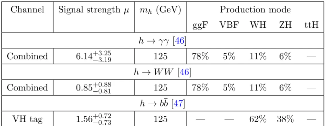
Channel Signal strengthµ mh (GeV) Production mode

ggF VBF WH ZH ttH

h_→γγ [46]

Combined 6.14+3.25₋_3.19 125 78% 5% 11% 6% —

h_→W W [46]

Combined 0.85+0.88_−0.81 125 78% 5% 11% 6% —

h_→b¯b [47]

VH tag 1.56+0.72_−0.73 125 — — 62% 38% —

Table 3. Tevatron results for up to 10 fb−1_at √_s_{= 1}_._{96 TeV, as employed in this analysis.}

it can be tensorial with a vertex_∝(gµν ₋qµ1q2ν

q1.q2), where q1,q2 are the momenta of the two

gauge bosons. The leading SM couplingsλW, λZ given in eqs. (2.8) and (2.9) are vectorial. Tensorial couplings are generated only at one-loop and are_O(α)_∼10−2_.

Once HDOs are taken into account, the relative importance of the vectorial and tenso-rial terms is modified. On one hand vectotenso-rial couplings are rescaled by the coefficientsaW,Z. On the other hand new tensorial contributions ζW,ζZ are generated following eq. (2.17). The amplitude associated to ahV V vertex (with theV’s possibly off-shell) is in general

M(hV V)λ1,λ2 ₌_eµ(∗)

λ1 e ν(∗) λ2

iaVλSMV gµν−i2ζVq1.q2

gµν₋q

µ 1q2ν

q1.q2

, (4.1)

where _M0,0 _and _M±,± _{are the longitudinal and transverse helicities amplitudes,} respec-tively. Interferences among helicity amplitudes then determine angular distributions (see e.g. [53]). In this work, we consider that the SM contribution to the tensorial coupling is small with respect to the one induced by New Physics. The relative magnitude of the longitudinal and transverse amplitudes in case of a vectorial coupling is given by

rv =

M0,0v

M±,±v

=

m2_h−q2₁−q2₂

2_|q1||q2|

, (4.2)

while it is the inverse in case of a tensorial coupling,

rt=

M0,0t

M±,±t

= 2|q1||q2| m2_h−q2₁−q2₂

. (4.3)

(13)

JHEP07(2013)065

To perform an exact analysis, one should redo the fits to LHC data taking into account the modified Lorentz structure in the expected signal. Such work is clearly beyond the scope of our present study. Instead we will show that under reasonable approximations we can useεSM+HDO=εSM in the present analysis.

There are three processes sensitive to the ζV tensorial couplings in the context of the searches for the Higgs boson at around 125 GeV: the leading decay to weak bosons

h _→ V V∗_{, and the VBF and VH production modes. We now discuss how we treat these} three tensorial contributions.

4.1 h_→V V∗

In the case of a light Higgs boson, the leading decay occurs with one of theV off the mass shell. The weak bosons then decay into fermions. For massless fermions, the kinematic bounds on the on-shell boson energyEV aremV < EV <(m2h+m2V)/2mhin the rest frame of the Higgs. Because of theV∗ _{propagator, the lower bound}_E

V =mV is favorized, imply-ing that both weak bosons are preferentially produced at rest. Longitudinal and transverse amplitudes are then equally populated, rv = 1. Therefore, one has rt = 1 as well, such that one can see qualitatively that a tensorial contribution cannot radically modify angular distributions. This is confirmed with the exact angular and invariant mass distributions among leptons induced by pure vectorial and pure tensorial couplings [54, 55].8 In our study, the tensorial contributions are constrained to be subleading with respect to the vectorial contributions, such that the deviations induced on angular and invariant mass distributions can be easily be smaller than the current statistical uncertainty. In addition, they could also be misidentified with the background. For example, inh_→V V∗, the distri-bution of the most discriminant observable, “lepton-oppositeZ momentum angle”, is very similar to the distribution of the irreducible backgroundqq¯_→ZZ∗ _{(see figure 3 in [}₅₆_]).

Following what discussed above, we can reasonably assume that angular and invariant mass distributions are not affected by the presence of tensorial couplings given the current level of precision. Polarization of the on-shell V can thus be averaged, and we are left with a matrix element scaling as

|M|2 =_|Mv+Mt|2 ∝

a_VλSM_V −2ζ_Vq₁.q₂

2

, (4.4)

where q1, q2 are the momenta of the two vector bosons. In the Higgs rest frame, one has

q1.q2 =mhEV −m2_V, which is bounded as

mV(mh−mV)< q1.q2<

m2 h−m2V

2 . (4.5)

The exact tensorial contributions to the total decay widths are given in appendix C. We introduce the dimensionless positive quantity

νV V =q1.q2/m2h, (4.6)

8_{Overall, the situation is much less striking than for a CP-violating contribution, which forbids the decay}

(14)

JHEP07(2013)065

withV _≡W, Z. Defining

hνV Vi=

R

νV VMvM∗tdP S

R

MvM∗tdP S

, _hν_{V V}2 _i=

R

ν2

V V|Mt|2dP S

R

|Mt|2dP S

, (4.7)

the vector-tensor interference term will be _∝ ζVhνV Vi and the pure tensor contribution will be _{∝ |}ζV|2hνV V2 i. For mh = 125.5 GeV, mZ = 91 GeV, mW = 80 GeV, one gets hνZZi= 0.2209, hνZZ2 i

1

2 = 0.2211, hν_WWi= 0.2653,hν2 WWi

1

2 = 0.2659. In the following we

will make the approximation _hν2

V Vi ≈ hνV Vi2.

4.2 VBF production mode

For the VBF process, both ATLAS and CMS apply hard cuts on the outgoing jets rapidities and their difference. The rapidity distributions of the two jets are similar in presence of a tensorial coupling, just like in the decay into two photons or in the production via gluon-gluon fusion, such that one can assume that cut efficiency is the same. The crucial change lies in the azimuthal angleφjj between the two tagging jets (see e.g. [53] and references therein). Indeed, both weak bosons are space-like, with virtualities considerably smaller than m2

h. Such values are favorized to balance the space-like V and the outgoing jets virtualities. As a result one has typically rv ≫ 1, rt ≪ 1 i.e. vectorial and tensorial amplitudes are mostly longitudinal and transverse, respectively. Consequently, the φjj distribution is almost flat for a pure vectorial coupling, and strongly peaked at π/2 for a pure tensorial coupling. For a large enough HDO contribution to the tensorial coupling, an anomalousφjj distribution could thus be observed. However, this variable is not used for the selection of the events in the experimental analyses we consider. Therefore, the selection efficiencies are also suitable in the case of large tensorial contributions, and one has εSM =εSM+HDO. One can average over the polarizations, and the squared amplitude is then simply rescaled by a factora_VλSM_{V BF} −2ζ_Vq₁.q₂

2 .

We still have to determine the magnitude of the tensorial contribution. In this process, the scalar product of the weak boson momentaq1.q2is related to the incoming and outgoing quarks as q1.q2 = m2_h/2 +p1.p3+p2.p4. The outgoing quarks are highly energetic with respect to the amount ofpT they receive from theV fusion, such that one has |p1| ≃ |p3|

and _|p2| ≃ |p4|. In terms of the p_T and rapidities of the outgoing quarks we have then

q1.q2 =

m2 h

2 +|pT,3|

21 +e−η3

2 +|pT,4|

21 +e−η4

2 . (4.8)

Without the tensorial contribution, the pT distribution peaks typically at values smaller than mV. The tails of the pT distributions drop quickly for higher energies [58], with typically one jet at a time getting a largepT [19]. One can thus assume q1.q2 ≈m2h/2 to a good approximation. Once the tensorial coupling is taken into account, a deviation from the expected SM distributions might be present in the high-pT tails, as q1.q2 is enhanced at large pT. However, as long as one counts the total number of events, i.e. the integral of the distribution, this enhancement ofq1.q2 has a small weight and can be safely neglected. Finally, defining the dimensionless positive quantity

νVBF=q1.q2/m2h, (4.9)

(15)

JHEP07(2013)065

4.3 VH production mode

In the case of the associated production with an electroweak gauge boson, the scalar product of the momenta of the weak bosons is given by

q1.q2 =

s+m2_V ₋m2_h

2 , (4.10)

where √s is the partonic center-of-mass energy, which is typicallys/m2_V =_O(100) at the LHC. Therefore, contrary to the two other processes, the product q1.q2 is large because it contains the partonic center of mass energy √s. The tensorial contribution is then substantially enhanced in this process. Besides, we have rv 6=rt, as rv =rt−1 ≈

√

s/2mV, such that the angular distributions may in principle be substantially modified by the presence of the tensorial coupling.

However, it turns out that for both polar and angular distributions, the angular effects can be neglected. We refer to [59] and references therein for the expressions. Although results are given fore+e−_{collisions, they can be trivially generalized in the case of the LHC.} For the distribution of the polar angle of the vector boson in the laboratory frame, it is the longitudinal component ofV which enters mainly, such that the tensorial contribution to the distribution is suppressed by an additional factor _O(m2_V/s). For the azimuthal distributions, the tensorial contributions can be sizeable, but the whole distribution tends to be flat for s_≫m2_V, with non-flat terms suppressed by powers ofmV/√s. As a result, although various pieces of angular information are used in event selection for this mode of production, we can safely neglect the angular effects of the tensorial coupling.

Concerning the magnitude of the tensorial contribution, it appears that it reduces to a simple rescaling _∝ λSM_V + 12ζVm2V in the limit s ≫ m2V. The rescaling is exact up to a subleading term _O(12m2

V/s) ≈ 0.1. To include the subleading s-dependent terms, an integration over the partonic density functions would be necessary.

5 Deviations caused by New Physics

5.1 Higgs signal strengths

Theoretical signal strengths for Higgs searches can be expressed as

ˆ

µ(X, Y) =

σ(X_→h)_B(h_→Y)εXY

SM+HDO [σ(X _→h)_B(h_→Y)εXY_]

SM

(5.1)

where _B is the branching ratio of the decay and the coefficient εXY _∈ [0,1] characterizes the efficiency of event selection for a given subcategory. In all generality, efficiencies in the SM with and without HDOs are not necessarily the same, i.e. εSM+HDO 6=εSM, because kinematic distributions can be modified in a non-trivial way by HDOs. The selection criteria calibrated on the SM expectations are then unadapted in such situation and complicates the interpretation of the signal strengths.

(16)

JHEP07(2013)065

searches. It is therefore a good approximation to setεSM+HDO=εSM. Thus, for each signal strength, one can simply incorporate the contributions coming from the tensorial couplings in the rescaling of the Standard Model signal strength.

The gluon-gluon fusion process is modified both by the tree-level HDO contribution ζg and the anomalous Higgs-fermion couplingscf. Keeping only the third generation, we get

σggF=σggFSM

ctλt,SMg +cbλb,SMg +ζg

λt,SMg +λb,SMg

2 . (5.2)

Vector boson fusion is modified by the anomalous vectorial couplings aW,Z and by ζW,Z. Denoting byλSM

VBF the effective SM couplings, one has

σVBF=σVBFSM

aWλSMW +aZλSMZ −2νVBFm2h(ζW +ζZ)

λSM W +λSMZ

2 . (5.3)

The parameter νVBF is defined in section 4.2. We take νVBF = 1/2. The associated production with an electroweak gauge boson is modified as

σVH =σVHSM

aVλSMV + 12ζVm2V

λSM V 2 , (5.4)

whereV =W, Z. Finally, the associated production with a t¯tpair is rescaled as

σttH =|ct|2σttHSM. (5.5)

The decays of the Higgs boson into fermions are modified as

Γf f =|cf|2ΓSMf f . (5.6)

The tree-level decays to vector bosons are modified as

ΓV V =

aV λSMV −2ζVm2hhνV Vi

λSM V 2

ΓSM_{V V} , (5.7)

where the parameter _hνV Vi, defined in eq. (4.7), encodes the modification of phase space integrals. Loop-induced decays are sensitive to more deviations,

Γγγ = ΓSMγγ

aWλW,SMγ +ctλt,SMγ +cbλb,SMγ +cτλτ,SMγ +ζγ

λW,SMγ +λt,SMγ +λb,SMγ +λτ,SMγ

2 , (5.8)

ΓZγ = ΓSMZγ

aWλW,SM_Zγ +ctλ_Zγt,SM+cbλb,SMZγ +cτλ τ,SM Zγ +ζZγ

λW,SM_Zγ +λt,SM_Zγ +λb,SM_Zγ +λτ,SM_Zγ

2 . (5.9)

(17)

JHEP07(2013)065

5.2 QCD radiative corrections

Many of the above described processes receive leading radiative corrections from QCD loops. For all the tree-level processes, the structure of loop diagrams is not modified by the insertion of HDOs, including the tensorial couplings, such that radiative corrections factorize up to higher order corrections. It is thus straightforward to take them into account, simply using the NLO predictions ofσSM _{and Γ}SM_.

The situation is more involved in the case of the loop-induced processes (h _→ γγ,

h_→ Zγ, andgg _→h) because this time the tensorial coupling is competing with the SM loops. Hence the effects of the ζ’s may be very large in these processes, such that it is important to properly take into account the radiative corrections. As stated in section 2, the HDOs implicitely contain higher-order corrections from irreducible SM loops. These contributions therefore have to be taken into account for the SM effective couplings and not for theζ couplings.9

The processes h _→ γγ and h _→ Zγ only receive virtual NLO QCD corrections. For

h _→ γγ, we take into account the exact values of the correction factor to the quark effective couplings

λq,SM_γ =λq,SM_γ _|LO

1 +αs

π CH(τq)

, (5.10)

where the CH function can be found in [19]. Forh → Zγ, one can take the correction in the heavy top limit as a good approximation [19],

λt,SM_γ =λt,SM_γ _|LO

1₋αs

π

. (5.11)

The situation is more subtle for the ggF process, because of the presence of important NLO real corrections. Introducing the tensorial coupling leads generally to non-trivial modifications of the integrals over parton densities for real emissions. However, in the heavy-top limit and neglecting the small bottom quark contribution, the QCD corrections to the SM loop and to the tensorial coupling ζg become similar and factorize. Adopting this fairly good approximation, the SM effective coupling are rescaled as

λt,SM_g =λt,SM_g _|LO

1 +11 4

αs

π

. (5.12)

5.3 S and T parameters

The electroweak precision observables are affected in the presence of the HDOs. At tree-level theS and T parameters are related to the HDO coefficients as follows:

α S =

2swcwαWB +sw2 αD+c2wα′D

v2

Λ2, (5.13)

α T =

−1₂α′_D2+

1 2α

′ D

v2

Λ2 . (5.14)

Moreover, the SM loops are modified by the HDOs. TheTparameter receives new divergent contributions from the modified SM couplings aZ and aW in eq. (2.13). A quadratic

(18)

JHEP07(2013)065

divergence,

α∆T =₋ Λ 2

16π2_v2

α′ D2v2

Λ2 , (5.15)

arises from custodial breaking [60]. Dropping other terms that are proportional toα′_D and

α′

D2 (that already appear at tree-level) the two couplings coincide and we can take the

result from ref. [5],

α∆T =₋ 3e 2

32π2_c2 w

α_D2−

1 2αD

v2 Λ2 log

m_h

Λ

. (5.16)

Similarly, the S parameter receives corrections due to the modified Higgs coupling αZ [5], hence it is expected to get new contributions proportional to αD2 and α′

D2. Finally, the

tensor couplings ζV can also generate new SM loop contributions which have been given in ref. [61],

α∆S= e 2

24π2

α_D2 +

1 2α

′ D2

v2 Λ2 log

m_h

Λ

+ e 2

2π2(αBB+αWW)

v2 Λ2log

m_h

Λ

. (5.17)

Finally we neglect the contraints coming from the W and Y parameters [50] as they are expected to have a small impact on our results.

6 Bayesian setup and low-Λ scenario

6.1 Bayesian inference

We are working in the framework of Bayesian statistics (see [15] for an introduction). In this approach, a probability is interpreted as a measure of the degree of belief about a proposition. Our study lies in the domain Bayesian inference, which is based on the relation

p(θ_|d,_M)_∝p(d_|θ,_M)p(θ_|M), (6.1)

whereθ_{≡ {}θ1...n}are the parameters of the modelM, andddenotes the experimental data. The distribution p(θ_|d,_M) is the so-called posterior probability density function (PDF),

p(d_|θ,_M)_≡L(θ) is the likelihood function enclosing experimental data, andp(θ_|M) is the prior PDF, which represents our a priori degree of belief on the parameters. The model_Mis in our case the Standard Model extended with higher dimensional operators. The likelihood is defined in section3(see eq. (3.2)) and the theoretical expressions for the HDO modified signal strengths are given in section 5. The prior PDF is discussed in the next subsection. The posterior PDF is the core of our results. Integrating the posterior over a subsetλ

of the parameter set θ_{≡ {}ψ, λ_},

p(ψ_|d,_M)_∝

Z

dλ p(ψ, λ_|M)L(ψ, λ), (6.2)

leads to inference on the parametersψ.

(19)

JHEP07(2013)065

between various HDO contributions can happen. Intrinsically, the regions of parameter space in which precise cancellations occur have a weak statistical weight, such that they are flushed away after integration. The results we will present can thus be considered as generic, i.e. free of improbable cancellations.

We will consider uniform (flat) priors for the quantities

βi≡αi

v2

Λ2 (6.3)

and demand_|βi|<1. Moreover, we will fix the cutoff scale to be Λ = 4πv. In the following we will justify these choices and argue that it ensures in particular convergence of the HDO expansion as well as perturbativity of the UV theory, and minimizes the dependence on the choice of the HDO basis.

6.2 Priors and low-Λ scenarios

The prior distributions associated to our parameters is a key feature of Bayesian inference. We follow the “principle of indifference” [62, 63] that maximizes the objectiveness of the priors. Once a transformation law γ = f(θ) irrelevant for a given problem is identified, this principle let us find the most objective prior by identifying pΘ ≡ pΓ in the relation

pΘ(θ)dθ=pΓ(γ)dγ.

The cutoff scale Λ is given a logarithmically uniform PDF,

p(Λ)_∝ 1

Λ. (6.4)

By doing so, all order of magnitudes are given the same probability density. Regarding the dimensionless coefficientsα, note that the choice of the HDO basis should be irrelevant for the conclusions of our study. Given that coefficients in different basis are related through linear transformations, the most objective prior to associate to each αi is the uniform PDF,10

p(αi)∝1. (6.5)

This choice of prior is well justified, however, one should keep in mind that other possibilities still exist.

Let us emphasize that in our general framework, the following hypotheses need to be scrutinized.

• Perturbativity of the HDO expansion, _|αi|/Λ2 <O(1/v2),

• Perturbativity of the couplings expansions in the UV theory, _|αi|<O(16π2),

• HDO generation by loops,

10_{Here the principle of indifference sets the shape of the PDFs but does not set the bounds. One can}

see that ranges onα’s are not conserved from one basis to another. In the scenario of democratic HDOs, this issue will be automatically solved, as one relies only on perturbativity of the HDO expansion to set the bounds onα’s. In the scenario of loop suppressedOF F’s, one takes advantage of a particular choice of

(20)

JHEP07(2013)065

• Custodial symmetry.

In the present work, we investigate scenarios of low-scale New Physics, with values of Λ going up to _O(4πv). We take custodial symmetry to be an exact symmetry of the theory. This forbids the presence of the operators_O′

D2 andO_D′ . As a consequence, one has aW = aZ ≡ aV and some contributions to the EW precision observables are suppressed including the potentially large quadratic divergence in T. Recall that _OWW, OWB, and OBB are all independently custodially symmetric. This generally implies that processes involving theW and Z are not identically rescaled, for instance

σWH

σSM WH

6

= σZH

σSM ZH

. (6.6)

Our approach goes therefore beyond the fits involving pure rescalings induced by anomalous couplings.

Over this range of Λ, perturbativity of the HDO expansion is the dominant con-straint as it requires _|αi| < Λ2/v2 which automatically implies |αi| < 16π2 and hence perturbativity of the couplings expansions in the UV theory.

When the HDOs are generated within a perturbative UV theory, none of the field strength — Higgs operators _OF F ≡ OWW, WB, BB, GG (see eqs. (2.2) and (2.3)) can be generated at tree-level. Because of our appropriate choice of basis, these loop-generated HDOs are exactly the ones associated with the tensorial couplings ζg,γ,Zγ. We will therefore distinguish between two scenarios, depending on whether or not the _OF F’s are loop suppressed with respect to the other HDOs. Given that tensorial couplings can play an important role, this distinction is particularly crucial. The two scenarios, denoted by I and II, are respectively dubbed “democratic HDOs” and “loop-suppressed _OF F’s”. The main features are summarized in table4. These two scenarios are generic, in the sense that they encompass all known UV models in addition to the ones not yet thought of. This implies that features predicted only by specific UV models — e.g. suppression of HDOs or precise cancellations between HDOs — will get a small statistical weight, as we consider the whole set of UV realizations. Finally, we emphasize that the interpretation of Λ as a true New Physics scale also depends at which order the whole set of HDOs is generated. For instance, in the R-parity conserving MSSM, the whole set of HDOs is generated only at one-loop order, such that the actual NP scale should be_O(4πΛ).

A parameterization particularly adapted to low-Λ scenarios is as follows. Defining the parameters

βi =αi

v2

Λ2, (6.7)

it follows that the β’s and Λ are independent, i.e. p(αi,Λ) = p(Λ)p(βi). The β’s prior is the uniform PDF over [₋1; 1], noted U(βi). The prior of Λ is p(Λ) ∝ Λ2n−1, where n is the number of β’s. In our case, n = 9 is large enough such that this prior is essentially peaked at Λmax,p(Λ)≈δ(Λ−Λmax). We have therefore

(21)

JHEP07(2013)065

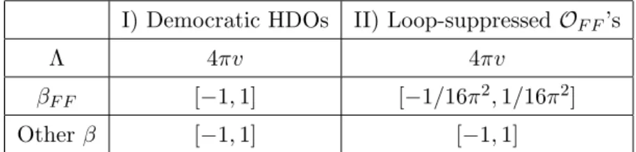
I) Democratic HDOs II) Loop-suppressed_OF F’s

Λ 4πv 4πv

βF F [−1,1] [−1/16π2,1/16π2]

Otherβ [₋1,1] [₋1,1]

Table 4. Summary of the setup of the scan in the two scenarios we consider. TheβF F ≡αF Fv2/Λ2

coefficients (whereF F =WW, W B, BB, GG) correspond to the field-strength — Higgs operators. In both cases we take custodial symmetry to be an unbroken symmetry.

This factorization allows us to marginalize over Λ, and to present our results in terms of β’s, which contain all the relevant information. A mild dependence on Λ will remain through loop-level_O(log Λ) terms in theSandT parameters, that will be discussed below. The fact that β’s prior is uniform and spans a constant range is essential to facilitate interpretation of the posterior PDFs. The fact that Λ_≈Λmax is also useful, as it renders straightforward the evaluation of the few Λ-dependent terms.

This parameterization turns out to be convenient in order to extract information about HDOs in a scale independent way, up to a mild _O(log Λmax) dependence. For example, for a given Λ, one can directly read the values of α’s on theβ’s plot. Similarly, for givenα’s, one can deduce the allowed Λ values from the plots. This parameterization is appropriate at low Λ, up to Λ = _O(4πv). Beyond this scale, the bound from HDO perturbative expansion competes with the bound from the perturbative expansion of the couplings. Once the latter dominates, the features of factorization no longer hold.

6.3 The MCMC setup

We evaluate posterior PDFs by means of a Markov Chain Monte Carlo (MCMC) method. The basic idea of a MCMC is setting a random walk in the parameter space such that the density of points asymptotically reproduces the posterior PDF. Any marginalisation is then reduced to a summation over the points of the Markov chain. We refer to [15,64] for details on MCMCs and Bayesian inference. Our MCMC method uses the Metropolis-Hastings algorithm with a symmetric, Gaussian proposal function. We run respectively 50 and 15 chains with_O(108_{) iterations each for the democratic HDOs case and the loop-suppressed} OF F’s case. Finally, we check the convergence of our chains using an improved Gelman and Rubin test with multiple chains [65]. The first 104 iterations are discarded (burn-in).

7 Inference on HDOs

(22)

JHEP07(2013)065

present is computed for Λ = 4πv_≈3 TeV. For smaller Λ, we expect the_∝log Λ constraints from ∆S and ∆T to mildly relax. We will comment below on this effect.

We will also discuss deviations from the SM cross sections and decay widths, defining

RX =

σX

σ_XSM, RY =

Γh→Y

ΓSM_h_→_Y , Rwidth= Γh

ΓSM_h , (7.1)

where X = ggF,VBF,WH,ZH,ttH, and Y = γγ, ZZ, Zγ, W W, b¯b, τ τ. Note that the observables are the signal strengths ˆµ(X, Y) rather than the individual RX and RY. Furthermore, the total width of the Higgs boson is about 4 MeV in the SM and cannot be probed directly currently at the LHC. The signal strengths, associated with a production mechanismX and a decay Y, can be expressed as

ˆ

µ(X, Y) =RX

RY

Rwidth

. (7.2)

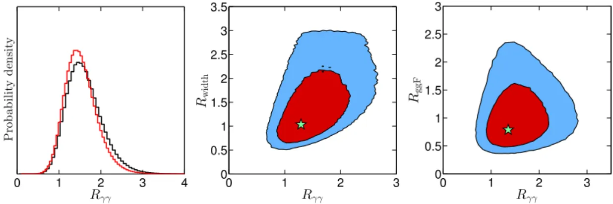
We present one-dimensional PDFs of the fundamental parametersβi for both scenarios in figure 1. Moreover, in table 5 we report the 68% and 95% Bayesian credible intervals (BCIs) for these quantities. We also present the BCIs for the other, dependent quantities, i.e. the anomalous couplingsaV andcf, the tensorial couplingsζi, and the variousR’s.

One can first remark that all of our HDO coefficients except βtand βb are constrained enough to stay within the bound _|βi| < 1, as required for the convergence of the HDO expansion. Furthermore, the βF F ≡βWW, W B, BB, GG coefficients are O(0.01) in both sce-narios. βD and βWB are strongly correlated in both scenarios as they appear in the S parameter at tree-level, see eq. (5.13) (we recall that we fix α′

D = α′D2 = 0 in order to

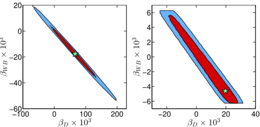
preserve custodial symmetry). We thus have 2cwβWB ≈ −swβD as can be seen in fig-ure2. The TGV observables also involveβD andβWB (see eq. (2.24)), and thus provide an independent constraint onβD(or equivalentlyβWB). The slight deficit inκγandg1Zas mea-sured by LEP, see eq. (3.1), tend to favors positive (negative)βWB (βD). Finally, note that in scenario II the PDF of βWB is limited to the [−1/16π2,1/16π2] range since we consider that the operator _OWB is loop-suppressed. This in turn fixes the allowed range forβD.

The β_D2 coefficient is allowed to deviate significantly from 0 as it only appears in

loop contributions to S and T and in aV. The probability of having βD2 > 0 is 94%

(90%) in scenario I (II) and comes fromT, as well as VBF and VH production modes and

h _→ V V decays. A value for aV > 1 leads to a positive contribution to T, as well as an enhancement of the VBF and VH production processes, the h_→V V∗ _{decays, and also to} the loop-induced decay rates,h_→γγ and h_→Zγ.

(23)

JHEP07(2013)065

−0.1 0 0.1 0.2 0.3

βD P rob ab il it y d en si ty

−0.4 0 0.4 0.8

βD2

P rob ab il it y d en si ty

−0.01 0 0.01

βGG P rob ab il it y d en si ty

−0.02 −0.01 0 0.01

βBB P rob ab il it y d en si ty

−0.08 −0.04 0 0.04

βW B

P ro b a b il it y d en si ty

−0.04 −0.02 0 0.02 0.04

βW W

−1 −0.5 0 0.5 1

βt P rob ab il it y d en si ty

−1 −0.5 0 0.5 1

βb P rob ab il it y d en si ty

−1 −0.5 0 0.5 1

βτ P rob ab il it y d en si ty

Figure 1. Posterior PDFs of the 9 fundamental parameters, βi ≡αiv2/Λ2, in scenario I (black)

and scenario II (red).

scenario II, and is also smaller if we take Λ<4πvdue to the log(mh/Λ) factor in eq. (5.17). We note that in scenario II the PDFs for βWW and βWB can easily reach the bounds set by the priors, while βBB is more strongly constrained by the data. This is due to the fact thatβBB enters inζγ with a coefficient roughly four times larger than the other two.

Finally, the Yukawa corrections parametrized by βf (f = t, b, τ) are much less con-strained as they only contribute to the rescaling factors cf, but account for most of the deviations of cf from 1, such that we often have |βf| ≫ |βD/4|and thus cf ≈ 1 +βf. It is worth noting that βt has a fairly large probability of being close to −1, which leads to small or vanishingct. The posterior PDF ofct is shown on the left pannel of figure 3.

(24)

JHEP07(2013)065

−100 0 100 200

−60 −40 −20 0 20

βD×103

βW

B

×

1

0

3

−20 0 20 40

−6 −4 −2 0 2 4 6

βD×103

βW

B

×

1

0

3

Figure 2. Posterior PDFs ofβWB versusβD in scenario I (left) and scenario II (right). The red

and blue regions correspond to the 68% and 95% Bayesian credible regions (BCRs). The green star indicates the maximum of our posterior PDF.

preference for small ct originates from the likelihood and not from a volume effect.11 The shapes of the PDF and profile likelihood for ct in figure 3 are in fact a direct consequence of the signal strength measurement µ(ttH, b¯b) by CMS [43], see table 2. Notice that the latter is so far the only analysis sensitive to the ttH production mode. In spite of its large error, the low central value drivesctefficiently to small values because of the relation RttH =c2t. Although small ct decreases (increases) the value of RggF (Rγγ), these changes can be compensated for without decreasing the likelihood. In the case

ct ≈ 0, the gluon-gluon fusion (ggF) process is mainly driven by the tensorial coupling

ζg ≡ βGG/v. We show in figure 4 the correlation between βGG and βt, which is needed to reproduce the observed ggF rate. For the decay h _→ γγ, we observe an increased rate Rγγ > 1, which can be seen in figure 5. Indeed, in the SM the h → γγ process is dominated by the W loops, and there is a destructive interference between the t and W

contributions. Therefore, the suppression ofcthelps increasing Rγγ. To better understand this enhanced rate, notice that naively combining the data in table 1–3 one obtains

µ(ggF + ttH, γγ) = 1.05_±0.28 and µ(VBF + VH, γγ) = 1.8_±0.6. It turns out that these different values are then realized with a slighly reducedRggF and an increasedRγγ.

The PDF ofβbis asymmetric with a longer right tail. βb appears mainly in theh→b¯b decay rate, i.e. in R_b¯_b.12 The reason of the asymmetry is the following: as the branching ratio_B(h_→ b¯b) = 57% in the SM, a deviation of βb from 0 (hence cb from 1) results in a sizeable modification of the total width of the Higgs. Our signal strengths are expressed as ˆµ(X, b¯b) =RXRbb¯/Rwidth and contain a strong correlation between Rb¯b and Rwidth. As

Rwidth significantly increases withRb¯b, the deviations fromµb¯b = 1 are smaller than what we could naively expect, allowing large values of R_b¯_b, hence βb. This explains the tails of the PDF of βb.

The 1D and 2D PDFs ofRwidthare shown in the left pannel of figure6. It turns out that a large increase ofRwidthis not forbidden by the measurements of other channels, in which

(25)

JHEP07(2013)065

scenario I scenario II

68% BCI 95% BCI 68% BCI 95% BCI

βD×103 [10,120] [−50,180] [−6,23] [−19,26]

β_D2×103 [70,350] [−50,480] [40,290] [−90,400]

βt×103 [−1000,110] [−1000,610] [−930,10] [−1000,590]

βb×103 [−10,530] [−220,930] [−110,500] [−280,860]

βτ×103 [−170,300] [−420,510] [−190,270] [−450,510]

βGG×103 [−3.2,8.0] [−4.0,9.6] [−3.3,0.6] [−4.2,2.7]

βWW ×103 [−19,7] [−30,18] [−5.6,2.3] [−6.0,5.6]

βWB×103 [−32,1] [−49,13] [−6.0,1.6] [−6.3,5.3]

βBB×103 [−12,0] [−17,4] [−1.7,1.6] [−2.9,3.0]

aV [1.02,1.15] [0.96,1.21] [1.02,1.14] [0.96,1.20]

ct [0.05,1.14] [0.03,1.63] [0.06,1.01] [0.04,1.60]

cb [0.90,1.54] [0.79,1.96] [0.89,1.50] [0.72,1.86]

cτ [0.84,1.31] [0.58,1.53] [0.81,1.27] [0.55,1.51]

ζgv×103 [−3.2,8.0] [−4.0,9.6] [−3.3,0.6] [−4.2,2.7]

ζγv×103 [−5.5,0.5] [−6.1,0.9] [−0.33,0.46] [−0.69,0.86]

ζZγv×103 [−13,18] [−18,30] [−4.9,4.4] [−7.6,7.9]

ζZv×103 [−20,2] [−31,11] [−3.4,2.3] [−5.1,4.4]

ζWv×103 [−39,15] [−59,37] [−11,5] [−12,11]

RggF [0.6,1.3] [0.5,2.0] [0.6,1.3] [0.4,2.0]

RVBF [1.0,1.4] [0.9,1.6] [1.0,1.3] [0.9,1.4]

RWH [0.7,1.3] [0.5,1.7] [1.0,1.3] [0.9,1.4]

RZH [0.7,1.2] [0.5,1.5] [1.0,1.3] [0.9,1.4]

RttH [0.02,1.0] [0.02,2.6] [0,0.9] [0,2.5]

Rγγ [1.1,1.9] [0.8,2.5] [1.1,1.8] [0.8,2.3]

RZγ [0,5.2] [0,12.0] [0,2.2] [0,4.3]

RZZ [1.0,1.3] [0.9,1.5] [1.0,1.3] [0.9,1.4]

RWW [1.0,1.3] [0.9,1.5] [1.0,1.3] [0.9,1.4]

R_b¯_b [0.7,2.2] [0.5,3.6] [0.7,2.1] [0.4,3.3]

Rτ τ [0.6,1.6] [0.3,2.2] [0.6,1.5] [0.2,2.1]

Rwidth [0.8,1.9] [0.7,2.7] [0.8,1.8] [0.6,2.5]

(26)

JHEP07(2013)065

0 0.5 1 1.5 2

ct P rob ab il it y d en si ty

0 0.5 1 1.5 2

ct P ro fi le L ik el ih o o d

Figure 3. On the left, posterior PDF ofctin scenario I (black) and scenario II (red). On the right,

profile likelihood along thectaxis in scenario I and scenario II (same color code).

−1 −0.5 0 0.5 1

−5 0 5 10 βt βG G × 1 0 3

−1 −0.5 0 0.5 1

−5 0 5 10 βt βG G × 1 0 3

Figure 4. Posterior PDF of βGG versusβtin scenario I (left) and scenario II (right). Color code

as in figure2.

0 1 2 3 4

R_γγ P ro b a b il it y d en si ty

0 1 2 3

0 0.5 1 1.5 2 2.5 3 3.5 R_γγ Rw id th

0 1 2 3

0 0.5 1 1.5 2 2.5 3 R_γγ RggF

Figure 5. On the left, posterior PDF ofRγγ in scenario I (black) and scenario II (red). Also shown

are the 2D posterior PDFs ofRwidth versusRγγ (middle) and RggFversus Rγγ (right) in scenario

I. Color code as in the previous figure.

this effect is compensated by an increase of the decay or production rates, in particular ggF. The upper bound on Rwidth,Rwidth.3, comes from the requirement βb <1.

(27)

JHEP07(2013)065

0 1 2 3

R_width P ro b a b il it y d en si ty

0 0.5 1 1.5 2 2.5 0 0.5 1 1.5 2 2.5 3 3.5 R_ggF Rw id th

Figure 6. On the left, posterior PDF of Rwidth = Γh/ΓSMh in scenario I (black) and scenario II

(red). Also shown is the 2D posterior PDF ofRwidthversusRggFin scenario I (middle) and scenario II (right). Color code as in the previous figures.

−8 −6 −4 −2 0 2

ζγv×103

−40 −20 0 20 40

ζZγv×103

−60 −40 −20 0 20 40

ζZv_×₁₀3

Figure 7. Posterior PDFs ofζγ, ζZγ, andζZ in scenario I (black) and scenario II (red).

rate. The PDF ofZγ is much broader because of the weak experimental sensitivity to the

Zγ rate. The distribution forζZ (and similarlyζW) is mainly due to indirect effects on the fundamental parametersβV V (γγandZγrates, as well as TGVs) rather than because of di-rect experimental constraints. Notice that even with the assumption of custodial symmetry (which enforcesaW =aZ), eq. (5.4) allows the rates for associated production to be differ-ent forZ andW because of the contribution of the tensorial couplings. It turns out thatζW andζZcan be large enough in scenario I to induce a substantial deviation fromRWH=RZH. This is shown in figure8. This effect is also present in scenario II to a lesser extent.

In scenario I, we observe two peaks of opposite signs for the tensorial couplings ζg and ζγ. These features appear because of the competition between the tree-level ζg,γ and the loop-level SM couplings in the ggF and digamma amplitudes. In addition to the classical region where ζ adds up to the SM coupling and cannot be very large, regions withζ =_O(₋2λSM_{) are also allowed. Note that} _ζ

γ is a linear combination of βWW, βWB,

(28)

JHEP07(2013)065

0 0.5 1 1.5 2

0.2 0.4 0.6 0.8 1 1.2 1.4 1.6

R_WH

RZ

H

0.8 1 1.2 1.4 1.6 0.8

1 1.2 1.4 1.6

R_WH

RZ

H

Figure 8. Posterior PDF of RZH versus RWH in scenario I (left) and scenario II (right). Color code as in the previous figures.

A feature of the PDF of ζZγ is that, in spite of the various constraints onβWW,βWB, andβBB, theZγrate is still likely to be considerably enhanced. The shape of theζZγ PDF is mainly constrained by the CMS bound ˆµZγ <9.3 in scenario I, while indirect constraints from theS parameter and trilinear gauge vertices dominate in scenario II. In the enhanced rate, the HDO contribution dominates, such that RZγ is mostly proportional to (ζZγ)2. This happens in scenario I, but also in scenario II although theζi are smaller. The PDF of the ratioRZγ can be seen in figure 9. The 95% Bayesian credible intervals are [0,12.0] for scenario I and [0,4.3] for scenario II. As large deviations are allowed in this channel within this framework, it is therefore particularly promising for the discovery of a NP signal.

In scenario I,ζZγ is sufficiently large to cancel the SM coupling, such that enhancement with both signs of ζZγ is realized. In contrast, for scenario II, only the branch with constructive interference ζZγ <0 can enhance RZγ. In both scenarios, ζZγ can cancel the SM coupling such that having a small or vanishing RZγ is likely.13

Finally, we compute the signal strength ofh_→Zγ in case of a fully inclusive analysis at the LHC. The PDFs are shown in the right panel of figure 9 for both scenarios. In scenario I, the distribution reaches the CMS 95% C.L. bound ˆµZγ <9.3, while it vanishes before in scenario II. The 68% and 95% BCIs are [0,3.6], [0,8.1] in scenario I and [0,1.6], [0,3.2] in scenario II.

Given that the 13/14 TeV LHC has a good potential to constrain theh_→Zγrate, one may wonder about the impact of a more precise measurement on our results. Therefore, we investigate the possibility of having ˆµZγ <2 at 95% CL, and we implement this bound as a step function.14 It mainly results in a better determination of βBB and βWW in both scenarios, as can be seen in figure 10. This new limit has an effect on the Higgs phenomenology in scenario I only. It leads to a slightly better prediction ofRWH: the 95% BCI is [0.7,1.5], instead of [0.5,1.7] when we take into account the current limit onh_→Zγ.

13_{We do not focus on this aspect as the direct searches at the LHC are still far from this level of precision.}

The shape of theRZγPDF follows the distribution of|ζZγ+λZγ|2, which presents a peak in 0. Schematically,

for a uniform distribution ofζZγ, the peak behaves asζ_Zγ−1/2. One can observe a similar behaviour forRttH. 14_{Note that the relative SM production rates}_σSM

X /

P

Xσ

SM

(29)

JHEP07(2013)065

0 5 10 15 20

RZγ

P

ro

b

a

b

il

it

y

d

en

si

ty

0 2 4 6 8 10

ˆ

µZγ

P

ro

b

a

b

il

it

y

d

en

si

ty

Figure 9. Posterior PDFs ofRZγ ≡Γ(h→Zγ)/ΓSM(h→Zγ) (left) and ˆµZγ (right) in scenario I

(black) and scenario II (red).

−20 −10 0 10

−40 −20 0 20 40

βBB×103

βW

W

×

1

0

3

−4 −2 0 2 4

−6 −4 −2 0 2 4 6

βBB ×103

βW

W

×

1

0

3

Figure 10. Posterior PDF ofβWW versusβBBin scenario I (left) and scenario II (right). The red

and blue regions correspond to the 68% and 95% BCRs from the current measurements, while the black and grey contours correspond to the 68% and 95% BCRs assuming in addition that ˆµZγ <2.

8 Conclusion

Less than one year after the first announcement of a signal in LHC data, the existence of a Higgs boson is at present firmly established. Time has come to probe in detail the structure of the now complete electroweak sector, searching for indirect signs of high-energy New Physics.

We use a complete basis of dimension-six operators encoding NP effects in an effective Lagrangian in which all tensorial couplings are taken into account. The basis is chosen such that field-strength — Higgs operators (_OF F) are exactly mapped into tensorial couplings. In this basis it is straightforward to study the well-motivated hypothesis of loop-suppression of these operators.

The data taken into account in our analysis are the whole set of results from ATLAS and CMS, including all available correlations, as well as Tevatron data. Trilinear gauge