The long memory behaviour of stock market volatility: evidence from the PIIGS countries

(1)

THE LONG MEMORY BEHAVIOUR OF STOCK MARKET

VOLATILITY: EVIDENCE FROM THE PIIGS COUNTRIES

Vasco Miguel de Assis dos Santos

Dissertation submitted as partial requirement for the conferral of Master in Finance

Supervisor:

Prof. Doutor Rui Menezes, Professor, ISCTE-IUL – Department of Quantitative Methods

Co-supervisor:

Prof. Doutora Sónia R. Bentes, Professor, ISCAL – Department of Finance

(2)

(3)

Spine

-T

H

E

L

O

N

G

ME

M

O

RY

BE

H

A

V

IO

U

R O

F S

T

O

CK

MA

R

K

E

T

VO

L

A

T

IL

IT

Y

:

E

V

ID

E

N

CE

FR

O

M

T

H

E

PIIGS C

O

U

N

T

RIE

S

V

a

sc

o

M

ig

ue

l d

e A

ss

is

d

o

s S

a

nto

s

(4)

II

Resumo

Neste estudo examinamos o comportamento de longa memória na volatilidade dos principais índices de mercado dos PIIGS: PSI20, FTSE MIB, ISEQ, FTSE/ATHEX e IBEX 35. Para realizar a nossa análise aplicámos dois modelos do tipo FIGARCH, um derivado por Baillie, Bollerslev e Mikkelsen (1996) e outro desenvolvido por Chung (1999). Adicionalmente, o Local Whittle Estimator foi também estimado.

Um conjunto de dados dos principais índices de mercado de acções dos PIIGS que inclui os preços de fecho diários desde 1 de Janeiro de 1998 até 8 de Março de 2013 foi utilizado.

Os resultados sugerem que, independentemente do modelo FIGARCH adoptado existem evidências de longa memória na volatilidade do mercado. No entanto, o Local Whittle Estimator revela que o processo de criação de dados é uma combinação de longa memória e saltos/quebras estruturais. Assim sendo, esta característica dos dados tem de ser tida em conta na construção de modelos de previsão de volatilidade.

Palavras-chave: Longa memória, Volatilidade, FIGARCH, Local Whittle Estimator JEL Classification System: G15; C13

(5)

III

Abstract

In this study we examine the long memory behaviour of stock market volatility of the PIIGS major indices: PSI 20, FTSE MIB, ISEQ, FTSE/ATHEX and IBEX 35. In order to conduct our analyses we apply two FIGARCH-type models, one derived by Baillie, Bollerslev and Mikkelsen (1996) and another one developed by Chung’s (1999). In addition the Local Whittle estimator is also computed.

A data set comprising the daily closing prices of the PIIGS’ major stock market indices spanning from 1st January 1998 to 8th March 2013 is used.

The results suggest that, irrespective of the FIGARCH model adopted, there is evidence of long memory in stock market volatility. However, the Local Whittle Estimator reveals that the data generating process is a combination of long memory and jumps/structural breaks. Therefore, this feature of the data has to be taken into account when constructing models for volatility prediction.

Key words: Long Memory, Volatility, FIGARCH, Local Whittle Estimator JEL Classification System: G15; C13

(6)

IV

Acknowledgements

First, I would like to express my gratitude to my supervisors, Professor Rui Menezes who helped and guided me; and to Professor Sónia Bentes, who also guided me, was always available when I had a question, and provided opinions, corrections and suggestions that were crucial to this study.

To my friend Cristiano Oliveira, I give the sincerest acknowledgment for the help and support.

To my parents and close family, I would like to say that I love you all and thank, especially to my mother for her efforts to bring me to this position.

(7)

V

List of Abbreviations

ADF: Augmented Dickey-Fuller;

ARFIMA: Autoregressive fractionally integrated moving average; ARMA: Autoregressive moving average;

BBM: Baillie, Bollerslev and Mikkelsen;

FIGARCH: Fractionally Integrated Generalized Autoregressive Conditionally Heteroskedastic;

GARCH: Generalized Autoregressive Conditional Heteroskedasticity;

IGARCH: Integrated Generalized Autoregressive Conditional Heteroskedasticity; KPSS: Kwiatkowski-Phillip-Schmidt-Shin;

(9)

VII

Sumário Executivo

O presente estudo visa proceder à investigação do comportamento de longa memória em cinco índices Europeus, PSI 20 (Portugal), ISEQ (Irlanda), FTSE MIB (Itália), FTSE/ATHEX (Grécia) e IBEX 35 (Espanha). A razão pela qual escolhemos estes índices foi motivada pela falta de investigação dedicada aos mesmos.

Uma série de dados apresenta longa memória se as observações que se encontram longe umas das outras estão fortemente correlacionadas, e as dependências entre observações sucessivas decaem a um ritmo lento. Este fenómeno teve as suas origens no Egipto, quando um consultor Hidrológico tentava desenvolver uma forma de prever as flutuações do fluxo do rio Nilo. Este desenvolveu um teste para detectar dependências de longo alcance, tendo encontrado correlações significativas de longo prazo entre as flutuações do fluxo do rio Nilo. As suas descobertas levaram outros autores a fazerem estudos em diferentes áreas, entre elas Economia e Finanças.

Para realizarmos este estudo aplicamos dois modelos FIGARCH e o Local Whittle Estimator. Os modelos FIGARCH aplicados foram o de Baillie, Bollerslev e Mikkelsen e o de Chung. Estes modelos têm uma grande flexibilidade para modelar a variância condicional uma vez que acomodam o modelo GARCH e o modelo IGARCH. O teste semi-paramétrico Local Whittle Estimator é um teste bastante robusto no que diz respeito às dinâmicas de curto prazo e permite formas muito gerais de dinâmicas de curto prazo, enquanto os modelos ARFIMA e FIGARCH são mais sensíveis às especificações utilizadas para representar estas dinâmicas. É também um teste simples e neste caso foi utilizado como um teste adicional ao FIGARCH.

Com os resultados obtidos com os modelos FIGARCH chegamos à conclusão que de facto existe longa memória na volatilidade dos índices estudados. Ao aplicarmos o Local Whittle Estimator, este sugere que embora exista longa memória na volatilidade não podemos descartar o facto de também poder existir saltos e/ou quebras estruturais no processo de criação de dados. Com isto em mente, ao construirmos os modelos de previsão de volatilidade não devemos ter apenas em conta a longa memória, mas também os saltos e/ou quebras estruturais.

(10)

1

1. Introduction

The interest in long memory does not find its roots in Finance/Economics as one should expect, but falls instead in the domain of a distinct branch of knowledge called Hydrology. It all started in 1906, when Harold Edwin Hurst, a civil servant, who went to Cairo, Egypt, as a hydrological consultant, faced the problem of how to predict the river Nile floods from year to year. He developed then a test for long-range dependence, having found significant long-term correlations among the fluctuations of the river Nile outflow, which were described in terms of a power law. His methodology is known today as the rescaled range statistics, range over standard deviation or R/S statistics. Later, Hurst published a series of papers, where he described his findings regarding to the long memory property (Hurst, 1951). After this seminal paper, several studies were conducted where the same pattern emerged. These studies were conducted in quite a few areas, such as, Biology, Climatology, Geophysics and on other natural sciences. For further details, the interested reader is referred to Mandelbrot and Wallis (1968) and MacLeod and Hipel (1978), inter alia.

Notwithstanding its origins there is a vast body of research on this topic in Finance, which covers several different areas, such as the volatility of stock market indices, currency, real estate and options. Fundamentally, a slow decay at a hyperbolic rate of its autocorrelation functions it is what characterizes a long memory series. In other words, the effects of volatility shocks decline over a long period, having long-lasting effects, which can be detected by analyzing measures of volatility, such as absolute returns and squared returns. On the other hand, a short memory process exhibits a rapid decline in its autocorrelation function so that unanticipated shocks affect the series for a short period. Long memory is essential for risk management, investment portfolios and pricing derivatives since it relates to the predictability of volatility.

Andersen and Bollerslev (1997a), demonstrated that the observed volatility process may exhibit long-run dependence, when they interpreted the volatility as a combination of several different short-run information arrivals. Thus, long memory property is an inherent feature of the return generating process, instead of the result of irregular structural shifts. The authors conducted a research on a one-year time series of five-minute Deutschemark-U.S. Dollar exchange rates. Ohanissian, Russel and Tsay (2005), derived a long memory test and applied it to intra-day foreign exchange data of

(11)

2 DM/$ and Yen/$. They concluded that volatility is a true long memory process. Lobato and Savin (1998) did not find any evidence of long memory in the returns. By contrast, they found strong evidence in the squared returns. Their analysis suggested that this evidence of long memory was real and not spurious. Liow (2009) analyzed 40 weekly real estate indices (original and hedged), having found long memory in the volatility structure of most securitized real estate markets. Additionally, Ding, Granger and Engle (1993), Baillie, Bollerslev and Mikkelsen (1996), Bollerslev and Mikkelsen (1996), Bollerslev and Wright (2000) and Bentes (2011), inter alia, found similar results.

However, some other authors challenged the evidence of long memory. They claimed that structural changes can cause long memory. This means that structural changes can explain the persistence in volatility and may produce a series that appears to exhibit long memory, which, in reality is not persistent. Based on a mixture model, a stochastic permanent break model and a Markov-switching model, Diebold and Inoue (2001) argue that structural changes in general and stochastic regime switching, in particular, are intimately related to long memory and easily confused with it, as long as a small amount of regime switching occurs in an observed sample path. Granger and Hyung (2004) show that occasional breaks generate slowly decaying autocorrelations and other properties of processes, where can be a fraction. They offer some theoretical arguments and simulation results, which substantiate the claim that it is difficult in practice to distinguish between the occasional breaks process and the process. In order to analyze the S&P 500 absolute stock returns two-time series models were used, an occasional-break model and an model.

Other authors believe that both long memory and structural breaks can coexist and explain the persistence in volatility. Choi, Yu and Zivot (2010) focused on the daily realized volatility of the Deutschmark/Dollar, Yen/Dollar and Yen/Deutschmark spot exchange rates with observed long memory behavior and found that structural breaks in the mean can partly explain the persistence on realized volatility. They based their analysis on a VAR-RV-Break model. Furthermore, Morana and Beltratti (2004) tested the existence of long memory and structural breaks in the realized variance process for the DM/US$ and Yen/US$ exchange rates. They showed that neglecting the breaking process is not necessary for extremely short forecasting periods once a long memory component is allowed into the model, but better forecasts can be obtained at longer horizons by modeling both long memory and structural change. Baillie, Han, Myers and Song (2006) examined the long memory behavior of both daily and high-frequency

(12)

3 intraday future returns for six key commodities. They found that long memory in volatility is a pervasive and consistent feature of commodity returns, not just being caused by shocks or regime shifts to the underlying price processes.

This research work aims to investigate the long memory behavior of five European stock indices, PSI 20 (Portugal), ISEQ (Ireland), FTSE MIB (Italy), FTSE/ATHEX (Greece) and IBEX 35 (Spain). What motivated one’s research was the lack of research devoted to the PIIGS countries.

To conduct one’s research, we first estimate the FIGARCH model proposed by Baillie, Bollerslev and Mikkelsen (1996), then the FIGARCH model derived by Chung (1999) and, finally, employ the Local Whittle Estimator.

The FIGARCH model has proven to be particularly useful in describing persistence. The semi parametric Local Whittle Estimator is also employed in order to produce an additional check for the presence of long memory. This estimator allows for quite general forms of short-run dynamics, whereas the ARFIMA and FIGARCH models are potentially sensitive to the specification used to represent the short-run dynamics (see Künsch, 1997 and Robinson, 1995). The same tests proposed by Shimotsu (2006) were used throughout one’s research.

In order to perform the previous test, we split the sample into subsamples and estimate (long memory parameter) for each subsample. Splitting the sample would lead to the same value of for each subsample as the one for the full sample or at least one close enough, given that the subsamples are sufficiently large. This property does not hold for spurious long memory processes, where the values of for the subsamples would be different than the of the full sample, and this difference would increase as the degree of sample splitting increases.

The second test is based on the differencing property of . Basically, we estimate for the whole sample, and then we use the estimate to take the th difference across the sample, and apply the KPSS test and the Phillip-Perron test to the differenced data and its partial sum. This seems to be a remarkably simple method, but provides a powerful tool to distinguish between the true process and the spurious one. Spurious long memory processes are or . Thus, taking their th difference would magnify its non- properties.

There are other alternative methods to account for long memory, such as, the Adaptive-FIGARCH of Baillie and Morana (2009), the two-step procedure of Morana

(13)

4 and Beltratti (2004) and the procedure derived by Ohanissian, Russel and Tsay (2005),

inter alia. However, the tests employed throughout this research work have some

advantages over the other ones. Firstly, there is no need for the identification of structural breaks when the underlying data generating process is unknown. Secondly, it is not necessary to enforce any restrictions on the types of structural breaks that can cause spurious long memory. Lastly, they are more detailed and fairly easy to implement, although their econometrics derivation seems to be more complex. However, they also have their shortcomings. We are only implementing Whittle-type long memory estimator. This means that, although it is computationally simple and straightforward, it is only just one type of long memory estimator.

The remainder of the paper is organized as follows. Section 2 defines Long Memory. Section 3 presents the methodological background. Section 4 describes the data. Section 5 and 6 discusses the empirical results obtained from the estimation of FIGARCH and the Local Whittle estimator, respectively. Finally, Section 7 concludes.

(14)

5

2. Long Memory

A time series is defined to exhibit long memory if observations far from each other are strongly correlated and dependence between successive observations decays at a slow rate. Specifically, this means that, with the presence of long memory, the market does not immediately respond to an amount of data flowing into the financial markets. Instead, it reacts slowly over time. With this in mind, to predict the future changes of prices we can use past prices as significant information. The main consequence of long memory is that shocks to the volatility tend to have long-lasting effects. Such persistence plays a vital role in risk management, investment portfolios and derivative pricing.

Harold Edwin Hurst was the first to discover this phenomenon while he studied the flow of the river Nile. Later, Hurst published a series of papers where he described his findings (Hurst, 1951). We can find other examples of the same phenomenon in biology, geophysics, climatology and other natural sciences. Some works that are worth mention are the works from Mandelbrot & Wallis (1968) and MacLeod and Hipel (1978).

Since then, the Hurst exponent, , has been calculated extensively for several time series, such as stock prices, stock indices, exchange rates and commodities. In the majority of the cases, a Hurst exponent of was found, indicating long memory correlation in the data.

Long memory can be expressed either in the time domain or in the frequency domain. In the time domain, long memory manifests itself as hyperbolically decaying autocorrelation functions. Therefore, observations far from each other are still strongly correlated and decay at a slow rate. A stationary process exhibits long memory or long-range dependence if the autocorrelation function at lag satisfies

_[ _] (1)

for some constants and . In contrast, a weakly stationary process has a short memory when its autocorrelation function is geometrically bounded

(15)

6 for .

Fox and Taqqu (1985) presented a more generalized definition of expression (1)

∑ | |

(3)

where denotes the number of observations.

In the frequency domain, the information comes as a form of a spectrum showing all the information within the interval - [ ]. In this matter, a stationary time series exhibits long memory if the spectral density behaves as

[ | | _] (4)

for some constants and .

There is a connection between expressions (1) and (4) and the Hurst exponent, , if , then and , which characterizes a classical long memory process. On the other hand, negative memory or antipersistence occurs when holds.

Alternatively, the memory of process can be expressed in terms of the behavior of its partial sum

∑

(5)

Rosenblatt (1955) defined short-range dependence in terms of a process that satisfies strong mixing so that the maximal dependence between two points within a process becomes trivially small as the distance between these points increases. Therefore, a process can be defined as having a short memory if

(6) exists and it is nonzero, and

[

] [ ]⇒ [ ] (7)

where [ ] denotes the integer part of , the standard Brownian motion and ⇒ the convergence in a distribution.

Resnick (1987) provided a definition of long memory that includes any process which has an autocovariance function for large such that

(16)

7 in which is any slowly varying function at infinity. Helson and Sarason (1967) demonstrated that any process with and the autocovariance function given by (8) violates the strong mixing condition, hence, it is a long memory process. Taqqu (1975) studied the weak convergence of a linear combination of a long memory process, where the weights are functions of Hermite polynomials. The study was conducted for a stochastic process ∑_{[ ]} , where is Gaussian with a zero mean and an autocovariance function obeying (8), , and is the th Hermite polynomial. For [ ()] then the normalized version of ∑_{[ ]} will converge to the Brownian motion. However, if [ ()] , the limit depend on , is non-Gaussian for and coincides with the Rosenblatt process when . Fox and Taqqu (1985) provided additional results for the quadratic form

∑ ∑

(9)

where are finite constants. Similarly, the normalized sum of the quadratic form converges either to a Brownian motion or to a Rosenblatt process. Furthermore, a vector of quadratic forms with a long memory converges to a vector of independent Gaussian random variables. In this case, the constants of the quadratic forms have to decay at sufficient speed to offset the long range dependencies in .

Finally, the most recent article, to the best of one’s knowledge is due to Diebold and Inoue (2001), who noted that there is a strong connection between the variance of partial sum definition and the spectral and autocorrelation of long memory.

All the definitions used in this section can be found in Bentes and Menezes (2013).

(17)

8

3. Methodology

3.1 FIGARCH Model

The Autoregressive Conditional Heteroskedastic (ARCH) processes were presented by Engle (1982), where he used this model to estimate the means and variances of inflation in the U.K.. These are mean zero, serially uncorrelated processes with non-constant variances conditional on the past, but constant unconditional variances. Accordingly with Engle (1982), the time-series and the associated prediction error are considered, where is the expectation of the conditional mean on the information set at .

A Generalized Autoregressive Conditional Heteroskedasticity (GARCH) model was proposed by Bollerslev (1986) and is as follows:

(10) where , and are polynomials in the lag operator of order and , respectively. Assuming that and for all , the GARCH ( ) model in Eq. (10) can be rewritten in the form of an ARMA( ) process:

[ ] (11)

where , and [ ] The process is interpreted as an innovation for the conditional variance, has a zero mean serially uncorrelated. In the GARCH model, the effect upon the past squared innovations on the current conditional variance decays exponentially with the lag length. This model presents some limitations since it assumes that the shocks decay at a fast geometric rate, thus only has short term persistence.

To overcome this problem it was developed the Integrated GARCH (IGARCH), by Engle and Bollerslev (1986) and can be written as follows:

[ ] (12) This model is characterized by having infinite memory. That is, the occurrence of a shock to the IGARCH volatility process will never die out. This feature may reduce its appeal to be used in asset pricing purposes, because this assumption would make the pricing functions for long-term contracts particularly prone to the initial conditions. To

(18)

9 overcome this Baillie, Bollerslev & Mikkelsen (1996) introduced the Fractionally Integrated Generalized Autoregressive Conditionally Heteroskedastic (FIGARCH). The FIGARCH ( ) model is given by:

[ ] (13) where is the fractional differencing parameter which measures the degree of long memory.

This model imply a slow hyperbolic rate of decay for lagged squared innovations in the conditional variance function, although the cumulative impulse response weights associated with the influence of a volatility shock on the optimal forecasts of the future conditional variance eventually tend to zero, this is a feature that the model shares with the weak stationary GARCH process.

This model has greater flexibility for modeling the conditional variance since it accommodates the covariance stationary GARCH model when and the IGARCH model when , as special cases. The advantage of the FIGARCH model is that, for , it is a lot more flexible to allow for an intermediate range of persistence. One of the disadvantages of the FIGARCH model is that it assumes strict stationarity but not weak stationarity.

Chung (1999) argues that Baillie, Bollerslev and Mikkelsen’s (1996) parameterization of the FIGARCH model may have a specification problem. He argues that the relations of BBM FIGARCH model with the ARFIMA models for the conditional mean are not perfect. The constant it is different than the constant in the ARFIMA models. This happens because the fractional integration operator exhibits an impact on , but it is irrelevant to . Additionally, for a given unconditional variance in , the parameter in equation (13) should be equal to zero regardless of the value of . With this in mind, Chung (1999) redefines the FIGARCH model as:

[ ] (14) the relationship between the parameter in equation (13) and the parameter is:

(19)

10

3.2. Local Whittle Estimation

In this section, we consider covariance stationary long memory processes. We assume the spectral density of the process satisfies:

₍₁₆₎

where ( ) and . The most widely used long memory process is a fractionally integrated process, given by

(17)

where is the lag operator and is a covariance stationary process whose spectral density is bounded away from zero at the zero frequency

The discrete Fourier transform ( ft) and the periodogram of evaluated at the fundamental frequencies can be defined as:

( ) ∑

( ) | ( )| (18)

Künsch (1987) and Robinson (1995) formulated the Local Whittle (Gaussian Semi Parametric) estimation. Robinson (1995) proposed a Gaussian objective function in terms of and ∑ [ ( ) ( )] (19)

where is the number of the periodogram ordinates and is some integer less than . The Local Whittle estimator ̂ of is obtained by minimizing (19), so that

( ̂ ̂)

[ ] (20)

where and are numbers such that . Concentrating Equation (20) with respect to , we have:

̂ [ ] (21) where ̂ ∑ ( ) ̂ ∑ ̂ (22)

The first test that we will apply is the sample Splitting-based diagnosis that was used by Shimotsu (2006).

(20)

11 We will split the samples into blocks, let be an integer and each block has observations. We also assume that is an integer. Define ̂ _{, to be}

the Local Whittle estimator of computed from the th block of the observations, { }.

The number of periodogram ordinates, , used in the objective function, has a crucial role in the Local Whittle estimator, since it determines the width of the frequency band used in estimating . We defined the number of periodogram ordinates used in the subsample as and we assume that is an integer. By doing the former, the subsample and the estimation of the entire sample will use an equal amount of frequency-domain information. This extenuates the effect of short-run dynamics on the test statistic since they have the same amount of bias from short-run dynamics.

For the th subsample, define

̂

[ ]

(23) where the objective function is constructed from the th block of the observations:

_̂ _∑ _{( ̃} ₎ (24) ̂ _∑ _̃ _{( ̃} ₎ ₍₂₅₎ _{( ̃} ₎ _| _∑ ̃ | (26) ̃ (27) To check for spurious long-memory processes, we estimate by taking the average of ̂ ̂ . A simple visual assessment can be done to check if we are in the presence of an process. If the average of ̂ ̂ it is close to the value of ̂,then is an process. This does not happen with spurious long memory. We also used the same assumptions on and , found in Robinson (1995) and Shimotsu (2006), they are the Assumptions A1-A4.

To formally testing true versus spurious , we use the same tests as Shimotsu (2006). This tests the hypothesis , where represents the number of subsamples, and are the true long memory parameters

(21)

12 for the full sample and each of the subsamples, respectively. Define a vector ̂ and matrix A as:

̂ ( ̂ ̂ ̂ ) ( ) (28)

Shimotsu (2006), show that, under ,

√ ̂ ( ) ( ) (29) where is a identity matrix and is a vector of ones. To test we use the adjusted Wald statistic. Here, we have the Wald statistic for testing as

̂ ( ̂ ) (30)

where denotes a generalized inverse of . Then has a chi-squared limiting distribution with degrees of freedom.

Hurvich and Chen (2000) reported that the finite sample variance of Local Whittle estimator tends to be larger than and the Wald test tends to over-reject the null hypothesis. They found out that replacing in the variance estimate by a number improves approximation, where is defined as:

∑ (31) ∑ ∑ (32)

Since as , this modification does not alter the asymptotic distribution of the test statistic. Following Hurvich and Chen (2000), Shimotsu (2006) introduced the adjusted Wald statistic:

̂ ( ̂ ) (33) One feature of this test is that each subsample-based estimator uses the same number of frequencies. This means that the bias of every elements of ̂ are the same and allows us to choose larger values of than in estimating . Here, we use the same assumptions introduced by Shimotsu (2006).

The second test is based upon the premises that, if an processes is differenced times, then the resulting time series are an process. This may seem simple, but some spurious long memory processes do not imitate this property. The

(22)

13 assumptions used here were the same used in Shimotsu (2006), and he shows that the th differenced series is:

̂ ̂₍ _{̂( ̂)) ∑} ( ̂ ) ( ̂) ( ̂( ̂)) (34) where ̂( ̂) ̅ ( ) (35) ̅ _∑ ₍₃₆₎

Once ̂ is calculated, it is then tested for unit roots. We also use the Phillips and Perron (1988) unit root test ( ) and the KPSS test (Kwiatkowski et al., 1992). Since the tests are now dependent upon the estimated ̂ instead of the true value, we must simulate their critical values, which are provided in Shimotsu (2006).

The Local Whittle estimator is quite robust to short-run dynamics. It allows for quite general forms of short-run dynamics, whereas ARFIMA and FIGARCH models are more sensitive to the specifications used to represent the short-run dynamics, Künsch (1987) and Robinson (1995). The long memory parameter from Local Whittle estimate is related to, but usually is not expected to be identical to the long memory parameter of the FIGARCH model. Semiparametric estimation has its own problems of being extremely data-intensive and generally exhibiting poor performance in terms of bias and standard errors. The main advantage of the Local Whittle estimate is its computational simplicity and the invariance of their limiting distribution with respect to .

(23)

14

4. Empirical Data

The data set comprises the daily closing prices of the PSI 20, FTSE MIB, ISEQ, FTSE/ATHEX and IBEX 35 indices, spanning from 1st January 1998 to 8th March 2013. Data was collected from the Thomson Reuters DataStream database.

To conduct one’s research the sample prices were converted into daily nominal percentage return series (not adjusted for dividends), given by

(

) (37)

for , where denotes the return at time t, the current price and the previous day’s price. Expression (37)can be rewritten as

[ ] (38)

According to Morana and Beltratti (2004), using daily data has the advantage that, from a statistical point of view, we gather a sample largely enough to make a statistically meaningful analysis. Also, from a practical point of view, daily returns are used by the financial industry and investors. Risk Management needs accurate forecasts of daily and weekly volatility for the implementation of value at risk models. In the case of quantitative asset allocation models, investors are interested in risk assessment at daily and sometimes even lower frequencies.

(24)

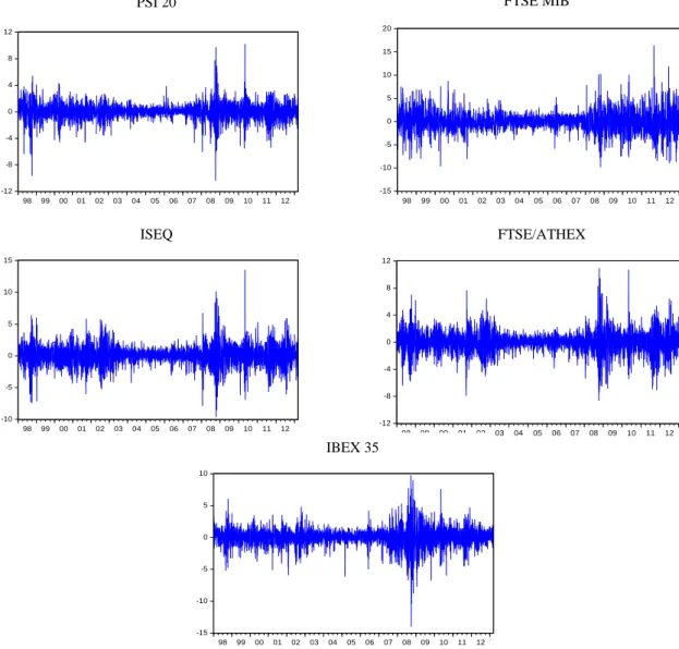
15 Fig. 1 gives us a visual representation of the daily log returns for the different indices. -12 -8 -4 0 4 8 12 98 99 00 01 02 03 04 05 06 07 08 09 10 11 12 Log Returns PSI 20 -15 -10 -5 0 5 10 15 20 98 99 00 01 02 03 04 05 06 07 08 09 10 11 12 Log Returns FTSE MIB -10 -5 0 5 10 15 98 99 00 01 02 03 04 05 06 07 08 09 10 11 12

Log ReturnsISEQ

-12 -8 -4 0 4 8 12 98 99 00 01 02 03 04 05 06 07 08 09 10 11 12 Log Returns FTSE/ATHEX -15 -10 -5 0 5 10 98 99 00 01 02 03 04 05 06 07 08 09 10 11 12 Log Returns IBEX 35

Fig. 1. Daily log returns of the PSI 20, FTSE MIB, ISEQ, FTSE/ATHEX and IBEX 35 indices in the period ranging from 1st January 1998 to 8th March 2013.

(25)

16

Table 1

Descriptive statistics and unit root tests for the PSI 20, FTSE MIB, ISEQ, FTSE/ATHEX, IBEX 35

PSI 20 FTSE MIB ISEQ FTSE/ATHEX IBEX 35

Mean _-0,00963 _-0,01063 _-0,00151 _-0,026193 _0,004518 Median _0,021168 _0,058486 _0,063955 _-0,01451 _0,071608 Maximum _10,19592 _10,87592 _9,733309 _16,37415 _13,48364 Minimum _-10,3792 _-8,59813 _-13,9636 _-9,796319 _-9,58587 Std. Dev. _1,225171 _1,590397 _1,447493 _2,10126 _1,583419 Skewness _-0,3035 _-0,07465 _-0,5401 _0,160014 _0,02991 Kurtosis _10,27641 _7,063915 _10,08522 _6,757199 _7,54639 Jarque-Bera _8557,005** _2654,988** _8208,059** _2247,781** _3303,238** Q(5) _46,257** _30,45** _17,087** _31,742** _23,39** Q(20) _88,353** _59,651** _47,889** _51,701** _50,121** Qs(5) _650,52** _1113,7** _1272,7** _533,39** _775,43** Qs(20) _1809,5** _3112,9** _3939,3** _1359,3** _2090,1** BG _6,524621** _3,901525** _2,931605** _4,017901** _3,417802** ADF _-56,2666** _-61,8669** _-58,3019** _-56,47721** _-45,663** PP _-56,2492** _-61,8766** _-58,2133** _-56,41895** _-61,0825** KPSS _0,107018 _0,200698 _0,188479 _0,559323 _0,10378

Notes: The Jarque-Bera corresponds to the test statistics for the null hypothesis of normality in sample returns distribution. The Ljung-Box statistics, Q(n) and Qs(n), seeks for the serial correlation in the return series and the squared returns up to the nth order, respectively. BG is the Breusch-Godfrey serial correlation test with 10 lags. For the tests ADF and PP the 1% critical value is -3,43186. The critical value for the KPSS test is 0,739 at the 1% significance level.

** Indicates a rejection of the null hypothesis at the 1% significance level.

Table 1 presents, the descriptive statistics and the unit root tests for all indices. As we can see, the samples means are remarkably small and only in the IBEX 35 the mean is positive, for the remaining indices the mean is always negative. The standard deviation is higher in comparison to the mean. The PSI 20 has the lowest standard deviation, thus being the index with the lowest level of volatility and the FTSE/ATHEX has the highest standard deviation, consequently being the index with the highest level of volatility. The returns are not normally distributed as indicated by the skewness, kurtosis and Jarque-Bera test statistics. The PSI 20, ISEQ and the FTSE MIB show

(26)

17 negative asymmetry, and the FTSE/ATHEX and IBEX 35 are positively skewed. All samples are leptokurtic with a kurtosis value higher than 3. The Jarque-Bera test statistics also show significant deviations from normality. The null hypothesis of the Ljung-Box Q statistics states that there is no serial correlation in the time series. We applied this test to the returns and squared returns with a lag of 5th and 20th order. Since the null is rejected at 1% significance level we conclude that there is significant evidence of serial dependence. The Breusch-Godfrey LM tests also reveal linear dependence.

We also performed three types of unit-root test: The Augmented Dickey-Fuller (ADF), Phillips-Perron (PP) and the Kwiatkowski-Phillip-Schmidt-Shin (KPSS). The tests ADF and PP null hypothesis checks if a time series contains a unit-root. Whereas, the KPSS tests it is used for testing a null hypothesis that an observable time series is stationary around a deterministic trend. All indices present a large negative number for the ADF and PP tests, rejecting the null hypothesis of a unit-root. In the KPSS test, we do not reject the null for any of the indices at a 1% significance level. Thus, the return series is a stationary process.

(27)

18

5. Empirical Findings

In order to remove any serial correlations present in the data, we first estimate an AR(p) model. By analyzing the correlogram plots for the return series, we chose an AR(1) for the ISEQ and FTSE/ATHEX, an AR(5) for the IBEX 35 and FTSE MIB, and finally an AR(7) for the PSI 20. The plots are not reported to save space. However, they are available upon request. Moreover, to verify the suitability of a time series model to account for the conditional mean we computed a number of diagnostic tests (Table 2).

Table 2

Residual's analysis for the fitted AR(p) model

Mean 1,62E-14 4,34E-12 -1,35E-10 -4,30E-12 -4,52E-11

Std. Dev. 1,215708 1,583554 1,445411 2,093298 1,578535 Skewness -0,192550 -0,127344 -0,500479 0,196303 -042479 Kurtosis 10,50615 6,829562 10,15679 6,78445 7,289270 Jarque-Bera 9050,275** 2361,162** 8335,869** 2286,637** 2937,14** Q(10) 7,4247 7,5947 16,018 11,708 9.8585 BG 1,087926 0,759622 1,534121 1,199055 1,188832 ARCH-LM 105,7523** 118,1778** 231,1330** 117,0364** 131,4875** Qs(10) 986,28** 1816,2** 2456,3** 969,76** 1401,7**

Notes: The diagnostic statistics Q(10) and Qs(10) are Ljung-Box statistics based on the first 10 autocorrelations of the standardized residuals and the autocorrelations of the squared standardized residuals respectively. BG is the Breusch-Godfrey serial correlation test with 10 lags. ARCH-LM refers to the ARCH-LM test of Homoscedasticity.

** Indicates a rejection of the null hypothesis at the 1% significance level.

As observed on Table 2, the Jarque-Bera test of the AR(p) residuals indicate non-normality. The PSI 20, ISEQ, FTSE MIB and the IBEX 35 display negative asymmetry, and the FTSE/ATHEX is positively skewed. All samples are leptokurtic with a kurtosis value higher than 3. Furthermore, the Ljung-Box and the Breusch-Godfrey are not statistically significant for all the indices, meaning that there is no serial correlation on the residuals. Finally, to check for heteroskedasticity, we employ the ARCH-LM test and the Ljung-Box statistics of the squared residuals, the null hypothesis of no Arch effects is rejected for all residual series at a 1% significance

(28)

19 level, finding which is corroborated by the rejection of the Ljung-Box test at the same significance level for the squared residuals.

Having fitted an AR(p) model in order to capture linear dependence in the mean and since there is evidence of ARCH effects in the residual series we proceed with the estimation of the FIGARCH model.

In the following sections, we present the results from the BBM’s FIGARCH model and Chung’s FIGARCH model. The FIGARCH ( ) and FIGARCH ( ) are the specifications that we are going to use in modeling the long memory property in the volatility of the five indices. The main advantage of the FIGARCH ( ) structure is that it parsimoniously decouples the long-run and short-run movements in the volatility. While the FIGARCH ( ) model nests a GARCH(1, 1) model, where shocks to the conditional variance either dissipates exponentially or persist indefinitely, for the FIGARCH ( ) model the response of the conditional variance to past shocks decay at a slow hyperbolic rate. Both these models are the most commonly used in empirical applications and also show satisfactory results. To estimate the FIGARCH model we used the OxMetrics6 software.

After that, we are going to present the Local Whittle Estimator. To perform the Local Whittle Estimator, we used the MatLab software and the same codes used by Shimotsu (2006).

(29)

20

5.1. BBM FIGARCH model

We begin by analyzing and comparing the BBM’s FIGARCH ( ) and FIGARCH ( ) specifications in modeling the long memory property in the volatility of the five indices. Table 3 and 4 report the results that we obtained under the Gaussian distribution.

Table 3

Estimation results of BBM FIGARCH (1,d,0) model under the Gaussian Distribution

0,060157** (0,013231) 0,036675* (0,017411) 0,072788** (0,016511) 0,052744* (0,024669) 0,062983** (0,018256) 0,047289** (0,014348) 0,043759** (0,011770) 0,081443** (0,024334) 0,134754** (0,033416) 0,059511** (0,015507) 0,311082** (0,078248) 0,567677** (0,070786) 0,334582** (0,069739) 0,328623** (0,045944) 0,552537** (0,11627) 0,438744** (0,064096) 0,592327** (0,068740) 0,403276** (0,060234) 0,387282** (0,037223) 0,588261** (0,11261) Ln(L) -5530,465 -6469,97 -6093,308 -7564,605 -6558,591 SIC 2,880051 3,366976 3,186342 3,996356 3,428994 AIC 2,873554 3,360481 3,179821 3,989776 3,422473 ARCH-LM 1,6910 1,0059 0,56628 0,38147 1,2111 Q(20) 92,531** 14,7462 28,4595 64,1971** 20,3975 Qs(20) 18,4619 30,4332* 14,3045 12,7253 29,8781

Notes: Standard errors based on QMLE are in parentheses below the corresponding parameter estimates. Ln (L) is the value of the maximized Gaussian log likelihood. SIC and AIC refer to the Schwarz Bayesian Information Criterion and Akaike Information Criterion respectively. ARCH-LM refers to the ARCH-LM test of heteroskedasticity. The diagnostic statistics Q(20) and Qs(20) are Ljung-Box statistics based on the first 20 autocorrelations of the standardized residuals and the autocorrelations of the squared standardized residuals respectively.

* Indicates the rejection of the null hypothesis at the 5% significance level. ** Indicates the rejection of the null hypothesis at the 1% significance level.

(30)

21

Table 4

Estimation results of BBM’s FIGARCH (1,d,1) model under the Gaussian Distribution

0,058701** (0,013233) 0,0306674* (0,017392) 0,072216** (0,016611) 0,053473* (0,024669) 0,063261** (0,018323) 0,031501** (0,011600) 0,037922** (0,013046) 0,062205 (0,035879) 0,102465* (0,032304) 0,046044** (0,016097) 0,167717* (0,065269) 0,034133 (0,041421) 0,096580 (0,11324) 0,100688 (0,060086) 0,072023 (0,044650) 0,503439** (0,075058) 0,587166** (0,056915) 0,456601** (0,16546) 0,440171** (0,074810) 0,600442** (0,064112) 0,481741** (0,062681) 0,584147** (0,058809) 0,436175** (0,083302) 0,407912** (0,039892) 0,578126** (0,069151) Ln(L) -5526,439 -6469,443 -6092,27 -7562,793 -6556,542 SIC 2,880104 3,368848 3,187951 3,997573 3,430077 AIC 2,871983 3,360729 3,1798 3,989348 3,421926 ARCH-LM 0,37577 0,31005 0,13256 0,37829 0,079429 Q(20) 91,6315** 14,6465 28,3321 63,077** 19,6795 Qs(20) 13,8702 30,3714* 13,6966 13,0005 29,4865*

Note: Standard errors based on QMLE are in parentheses below the corresponding parameter estimates. Ln (L) is the value of the maximized Gaussian log likelihood. SIC and AIC refer to the Schwarz Bayesian Information Criterion and Akaike Information Criterion respectively. ARCH-LM refers to the ARCH-LM test of heteroskedasticity. The diagnostic statistics Q(20) and Qs(20) are Ljung-Box statistics based on the first 20 autocorrelations of the standardized residuals and the autocorrelations of the squared standardized residuals respectively.

As shown in the previous tables, the parameter and are positive and found highly significant. Regarding the parameters and , we arise at a different pattern, that ranges from no significance, to 1% or 5% significance level.

The FIGARCH ( ) values span from 0,387282 for the FTSE/ATHEX to 0,592327 for the FTSE MIB, rejecting the null hypothesis of GARCH ( ) and IGARCH ( ) models at the 1% significance level. Therefore, these findings are consistent with a long memory process. Regarding the FIGARCH ( ) values, they span from 0,407912 for the FTSE/ATHEX to 0,584147 for the FTSE MIB, also

(31)

22 rejecting the null hypothesis of GARCH ( ) and IGARCH ( ) models at the 1% significance level. These results are as well consistent with a long memory process.

The results indicate dependencies between distant observations in the indices, which can be used to predict future volatility values. Such findings provide evidence against the efficient market hypothesis of Fama (1970). The efficient market hypothesis of Fama suggests that it is impossible to make any predictions from the past patterns and that the stock returns display a random walk.

The FTSE/ATHEX Index which is the most volatile according to the standard deviation results, it is the one that exhibits the lowest persistence. Nevertheless, the Index that presents the higher persistence is not the one who has the lowest volatility. The PSI 20 is the lowest volatile Index, and his value is 0,438744 and 0,481741 according to the estimates of the FIGARCH ( ) and FIGARCH ( ) respectively. In the study of Bentes (2011), it is found an inverse relation between these two measurements, which might be explained by the fact that smaller markets are characterized by being less liquid, thus are less efficient in the sense of the EMH. Therefore, exhibiting higher persistence, this is consistent with the findings of Di Matteo, Aste and Dacorogna (2003) and Grau-Carles (2000). However, here we do not verify that.

Comparing both models, the FIGARCH ( ) model ensures the positivity constraint in the conditional variance, Baillie, Bollerslev and Mikkelsen (1996) considered that these conditions, and , as necessary and sufficient to ensure for the conditional variance of the FIGARCH ( ) model to be positive almost surely for all . Additionally, FIGARCH ( ) specification provides a better representation of a long memory volatility process, since the parameter is insignificante in the majority of the cases, only in the PSI 20 the parameter is significant at the 5% level. The FIGARCH ( ) in the majority of the cases presents a lower SIC value. The Ljung-Box statistic results are quite similar in both models. The ARCH-LM test does not reject the null hypothesis in any of the models. Finally, the AIC test results do not clearly show which one it is the best. Therefore, the FIGARCH ( ) model is superior to the FIGARCH ( ) model in capturing the long memory property of the volatility in these five indices stock returns.

(32)

23

5.2. Chung’s FIGARCH model

In this section, we analyze and compared the Chung’s FIGARCH ( ) and FIGARCH ( ) specifications in modeling the long memory property in the volatility of the five indices like we did in the previous section. Table 5 and 6 report the results that we obtained under the Gaussian distribution.

Table 5

Estimation results of Chung’s FIGARCH (1, d, 0) model under the Gaussian Distribution

0,059728** (0,013160) 0,037344* (0,017617) 0,072942** (0,016410) 0,053066* (0,024278) 0,063508** (0,018567) 2,431853* (1,2385) 3,135498* (1,3007) 2,236646** (0,73320) 5,677339* (2,8476) 3,128599* (1,3820) 0,347249** (0,067095) 0,511769** (0,04638) 0,34626** (0,050734) 0,391246** (0,060375) 0,46485** (0,045630) 0,47550** (0,050243) 0,536481** (0,041103) 0,411356** (0,040358) 0,451420** (0,051136) 0,501373** (0,045630) Ln(L) -5530,433 -6471,201 -6093,517 -7566,581 -6560,112 SIC 2,880034 3,367617 3,186451 3,997398 3,429786 AIC 2,873537 3,361122 3,17993 3,990818 3,423266 ARCH-LM 1,8213 1,2578 0,56017 0,46136 1,3916 Q(20) 89,9195** 14,7445 28,327 64,9674** 20,0857 Qs(20) 18,0548 31,0886* 14,4141 13,7481 33,8839*

(33)

24

Table 6

Estimation results of the Chung’s FIGARCH (1, d, 1) model under the Gaussian Distribution

0,058509** (0,013204) 0,037011* (0,017615) 0,072166** (0,016649) 0,054056* (0,024263) 0,063314** (0,018665) 2,359133* (1,1790) 2,792068* (1,2392) 2,231773** (0,74663) 5,878645* (2,9204) 2,838265* (1,2400) 0,160543* (0,066382) 0,046001 (0,040104) 0,091116 (0,11615) 0,098942 (0,055597) 0,086962* (0,042495) 0,513506** (0,068603) 0,556127** (0,049074) 0,446628** (0,15230) 0,500177** (0,077096) 0,555900** (0,055116) 0,500339** (0,046073) 0,542068** (0,037949) 0,430866** (0,057639) 0,474645** (0,051826) 0,517884** (0,041860) Ln(L) -5526,502 -6470,307 -6092,566 -7564,409 -6557,56 SIC 2,880137 3,369296 3,188107 3,998425 3,43061 AIC 2,872016 3,361177 3,179956 3,9902 3,422459 ARCH-LM 0,41372 0,27933 0,13360 0,35013 0,087853 Q(20) 89,7654** 14,6274 28,1595 63,489** 19,4692 Qs(20) 13,7369 30,8596* 13,7058 13,9467 31,9707*

Commonly like in BBM’s FIGARCH models, in the Chung’s models the and parameters are positive and found highly significant. Regarding the parameters and , we arise at a different pattern, that ranges from no significance, to 1% or 5% significance level.

The FIGARCH ( ) values span from 0,411356 for the ISEQ to 0,536481 for the FTSE MIB, rejecting the null hypothesis of GARCH ( ) and IGARCH ( ) models at the 1% significance level. Thus, these findings are as well consistent with a long-memory process. Regarding the FIGARCH ( ) values, they span from 0,430866 for the ISEQ to 0,542068 for the FTSE MIB, also rejecting the null

(34)

25 hypothesis of GARCH ( ) and IGARCH ( ) models at the 1% significance level. Hence, the results are as well consistent with a long-memory process.

These results like in the BBM’s case display dependencies between distant observations in the indices, which can be used to predict future volatility values. Therefore, such findings provide once again proof against the efficient market hypothesis of Fama (1970). However, here we do not observe the same relationship that we observed with the BBM’s FIGARCH, where the highest volatile market had the lowest persistence estimate. With this model, that relationship does not seem to hold.

Comparing the two models, the FIGARCH ( ) it is superior to the FIGARCH ( ), for particularly the same reasons that we saw in the BBM’s case. The parameter is insignificant is the majority of the cases, the SIC value is lower in the majority of the cases for the FIGARCH ( ) and this model ensures the positivity constraint in the conditional variance.

Comparing the BBM’s model with the Chung’s Model, the values have an higher amplitude using the BBM’s FIGARCH model. In the case of the ARCH-LM, SIC, AIC and Ljung-Box statistics, the results are quite similar. In the end, both models arise to the same conclusion that there is evidence of long memory features in the volatility of the indices.

(35)

26

6. Local Whittle Estimator

To perform the Local Whittle Estimator, we used the MatLab software and the same codes used by Shimotsu (2006).

Table 7, 8, 9, 10 and 11 show the estimates for ̂ and ̅, the value of , and ̂ statistic from the log returns, for different values of , spaning from 200 to 800 and .

Table 7

Estimation and test results with PSI 20 log returns

̂ ̅ ̂ 200 0,588 0,5918 0,617 0,2322 1,5133 -1,9928 0,0507 300 0,533 0,5386 0,5568 0,6936 3,3043 -2,0247 0,0626 400 0,5423 0,548 0,5602 1,0678 2,5089 -1,974 0,0652 500 0,5368 0,5443 0,5492 3,0989 5,4273 -1,9413 0,0731 600 0,5268 0,533 0,5362 2,5601 5,9357 -1,9335 0,0792 700 0,5359 0,5424 0,5506 4,0814* 11,4662* -1,8671 0,0824 800 0,5375 0,5406 0,5494 2,032 8,1858* -1,8166 0,0884

Note: * Indicates the rejection of the null at the 5% level.

Table 8

Estimation and test results with ISEQ log returns

̂ ̅ ̂ 200 0,5144 0,5169 0,5526 0,0018 0,1656 -1,624 0,1107 300 0,5185 0,5335 0,5449 0,8382 3,0153 -1,7277 0,1004 400 0,5044 0,5151 0,5175 0,464 1,5552 -1,7613 0,0972 500 0,5014 0,5122 0,5214 0,6027 1,9517 -1,7673 0,0981 600 0,4943 0,4998 0,5118 0,284 1,3636 -1,7391 0,1025 700 0,5018 0,5113 0,5158 1,1812 5,082 -1,7555 0,1043 800 0,5108 0,5226 0,5269 1,9337 7,6387 -1,8018 0,1047

(36)

27

Table 9

Estimation and test results with IBEX 35 log returns

̂ ̅ ̂ 200 0,5372 0,5406 0,5649 0,1742 0,751 -2,3255 0,0766 300 0,4755 0,4778 0,49 0,0063 0,8817 -1,9772 0,0991 400 0,4682 0,4752 0,4847 0,4302 2,1514 -2,0007 0,1 500 0,4568 0,4636 0,4756 0,6555 1,8691 -1,9993 0,1004 600 0,4478 0,4494 0,4596 0,000059247 3,6645 -1,9901 0,1013 700 0,4463 0,4525 0,4606 1,2362 6,1001 -1,9653 0,1065 800 0,451 0,4542 0,4622 0,3308 3,6436 -1,9808 0,1109

Table 10

Estimation and test results with FTSE MIB log returns

̂ ̅ ̂ 200 0,5617 0,5559 0,5732 0,8763 2,5804 -1,3732 0,1212 300 0,5171 0,5121 0,517 0,0115 4,6819 -1,3616 0,1788 400 0,5104 0,5082 0,5125 0,0034 6,4451 -1,4051 0,1812 500 0,4952 0,496 0,4986 0,5296 4,1384 -1,3821 0,1879 600 0,4879 0,4848 0,4866 0,054 6,5574 -1,3701 0,1937 700 0,4862 0,4881 0,4878 1,3505 7,864* -1,3594 0,2041 800 0,4863 0,4862 0,4886 0,5686 4,7829 -1,3835 0,2108

(37)

28

Table 11

Estimation and test results with FTSE/ATHEX log returns

̂ ̅ ̂ 200 0,6036 0,589 0,6182 2,2199 1,9213 -0,9852 0,2416 300 0,5518 0,539 0,5573 1,2366 1,5062 -0,8426 0,2756 400 0,5459 0,5398 0,5555 0,2733 2,314 -0,9128 0,2626 500 0,5359 0,5315 0,5511 0,5334 3,6528 -0,9708 0,2502 600 0,5295 0,5287 0,5449 0,0079 5,2558 -0,9902 0,2477 700 0,5302 0,5339 0,5385 0,4447 3,8927 -1,0171 0,2472 800 0,53 0,5322 0,5425 0,1999 5,0637 -1,0451 0,2472

In all the indices, the value of ̂ and ̅ are close to each other, both ̂ and ̅ decrease as increases, this suggests that there is a possibility of presence of jumps and/or structural breaks in the data. The test rejects the null of the constancy of on the PSI 20 when and , when and and for the FTSE MIB when and . The and ̂ statistics do not present rejections of a stationary ̂th differenced series.

Overall, the results here presented do not support a true long memory process. However, the evidence of spurious long memory is not compelling enough as it would be if long memory was generated only by structural breaks. So we can arrive at the conclusion that long memory and jumps and/or structural breaks co-exist in all the indices under the study.

In table 12, 13, 14, 15 and 16, we divided the data from the indices into three subperiods of equal length and applied the same tests applied in the previous section to each of the subperiod to make an additional check. As it was mentioned before, splitting the sample would lead to the same for each subsample as the one for the full sample or at least one close enough, given that the subsamples are sufficiently large. This property does not hold for spurious long memory processes, in which the values of for the subsamples would be different than the of the full sample, and this difference would increase as the degree of sample splitting increases. Therefore, we are going to see if this happens.

(38)

29

Table 12

Estimation and results with PSI 20 log returns

̂ ̅ ̂ Subperiod 1: 40 0,6626 0,6197 0,7244 0,0651 0,7147 -0,6964 0,0753 100 0,5825 0,5471 0,5706 0,0038 0,311 -0,3398 0,1716 160 0,6124 0,5932 0,5869 0,2846 0,4225 -0,2062 0,1974 Subperiod 2: 40 0,5929 0,5565 0,7054 0,3819 0,9304 -2,1017 0,1696 100 0,5778 0,5671 0,6247 0,2088 1,3814 -1,771 0,1403 160 0,5612 0,5393 0,5679 0,743 2,5331 -1,7529 0,1286 Subperiod 3: 40 0,5877 0,62 0,6648 0,0029 1,163 -2,673 0,0744 100 0,4634 0,4757 0,522 0,0034 2,9548 -2,0033 0,0734 160 0,4861 0,4903 0,5246 0,0451 0,5956 -2,1885 0,068

Note: * Indicates the rejection of the null at the 5% level. Table 13

Estimation and results with ISEQ log returns

̂ ̅ ̂ Subperiod 1: 40 0,5535 0,5898 0,567 0,9255 1,811 -1,6756 0,1619 100 0,5761 0,5995 0,5837 2,0373 2,1113 -1,7963 0,1977 160 0,5393 0,5457 0,5281 0,537 3,0203 -1,3812 0,2919 Subperiod 2: 40 0,5462 0,5296 0,568 0,9957 1,7496 -1,1281 0,2877 100 0,4648 0,5081 0,545 0,2742 4,0898 -1,3007 0,2399 160 0,4729 0,5167 0,5442 0,2235 1,6996 -1,461 0,2141 Subperiod 3: 40 0,6929 0,6866 0,5189 0,2811 4,5729 -3,0837* 0,1762 100 0,4892 0,4782 0,4297 0,0093 0,3289 -1,0748 0,2277 160 0,4868 0,4732 0,4451 0,1257 3,3944 -1,1902 0,2109

(39)

30

Table 14

Estimation and results with IBEX 35 log returns

̂ ̅ ̂ Subperiod 1: 40 0,6593 0,601 0,6528 1,5503 2,2773 -1,178 0,0775 100 0,4982 0,4667 0,5404 0,003 3,4435 -0,4732 0,3854 160 0,5212 0,4969 0,5448 0,0472 1,5715 -0,5439 0,4332* Subperiod 2: 40 0,4301 0,3707 0,541 1,5342 2,1416 -1,7029 0,0851 100 0,4781 0,4735 0,5351 1,7172 5,4977 -1,6271 0,1404 160 0,4632 0,4704 0,4946 1,179 2,1754 -1,5468 0,1651 Subperiod 3: 40 0,5326 0,5627 0,5565 0,4736 0,4201 -2,8497* 0,0453 100 0,4366 0,4429 0,4577 0,003 2,1748 -2,2891 0,0562 160 0,4349 0,4395 0,4502 0,1473 0,6931 -2,2847 0,0605

Note: * Indicates the rejection of the null at the 5% level. Table 15

Estimation and results with FTSE MIB log returns

̂ ̅ ̂ Subperiod 1: 40 0,5418 0,4894 0,5807 0,0573 0,7405 -0,4581 0,3647 100 0,5521 0,53 0,5641 0,0273 2,8373 -0,5545 0,3434 160 0,549 0,5343 0,5533 1,5723 4,0111 -0,4882 0,4177 Subperiod 2: 40 0,4363 0,4165 0,4337 1,4184 2,3055 -1,6256 0,209 100 0,4305 0,4178 0,4484 3,5008 7,8018 -1,4795 0,2189 160 0,4254 0,4402 0,4688 3,021 5,7301 -1,5272 0,2073 Subperiod 3: 40 0,5483 0,5829 0,6004 0,0101 0,7479 -2,989* 0,0424 100 0,4799 0,4919 0,507 0,0051 1,7925 -2,5209 0,0531 160 0,495 0,4992 0,5003 1,6605 1,6907 -2,6659 0,0566

(40)

31

Table 16

Estimation and results with FTSE/ATHEX log returns

̂ ̅ ̂ Subperiod 1: 40 0,6771 0,5359 0,5334 2,1119 3,254 -1,0914 0,3228 100 0,521 0,4629 0,4806 0,038 2,537 0,0214 0,5688* 160 0,5207 0,5155 0,5208 1,7212 4,5612 0,0721 0,5918* Subperiod 2: 40 0,5043 0,4301 0,4884 0,3957 3,4742 -2,3961 0,0812 100 0,5254 0,5434 0,5601 2,7365 1,933 -2,2441 0,1005 160 0,5312 0,5545 0,5608 1,8276 2,4487 -2,1549 0,1405 Subperiod 3: 40 0,6115 0,6397 0,7201 0,7737 0,6051 -1,9155 0,056 100 0,5395 0,5517 0,5679 0,1376 0,3319 -1,8863 0,0704 160 0,5359 0,5454 0,5681 0,1123 0,7404 -1,9101 0,0774

The estimates of are different across subperiods mainly because of sampling variation and small values. The and ̂ statistics do not reject the null of a stationary ̂th differenced series for the majority of the cases, and the test does not reject the null for any of the indices.

Again, these results do not show strong evidence of a true long memory process in the volatility of the indices. They also suggest that there is a possibility of presence of jumps and/or structural breaks in the data, but they are not strong enough so that we could argue that we are in the presence of a spurious long memory process.

Overall, results of the Local Whittle Estimator do not show that we are in the presence of a pure long memory process, but they also do not support the opposite view that structural breaks account for all the observed persistence.

(41)

32

7. Conclusion

In this study we examine the long memory behavior of stock market volatility of the PIIGS major indices: PSI 20, FTSE MIB, ISEQ, FTSE/ATHEX and IBEX 35. To achieve this, we applied two FIGARCH-type models, one proposed by Baillie, Bollerslev and Mikkelsen, and the other by Chung, and the semi parametric Local Whittle Estimator to the indices.

A preliminary analysis uncovers non-normality, serial correlations and heteroskedasticity in all indices. As a consequence, we fitted an AR(1) for the ISEQ and FTSE/ATHEX, an AR(5) for the IBEX 35 and FTSE MIB, and finally a AR(7) for the PSI 20. A diagnostic analysis of the residuals shows that the serial correlation is no longer present in all the indices. Additionally, the ARCH-LM test and the Ljung-Box statistic of the squared residuals unfold heteroskedasticity. Having fitted an AR(p) model in order to capture linear dependence in the mean and since there is evidence of ARCH effects in the residual series we proceed with the estimation of the FIGARCH model.

Analyzing the results from the BBM’s and Chung’s FIGARCH models, we can see that the FIGARCH ( ) is superior to the FIGARCH ( ) model in capturing the long memory property of the volatility in the five indices stock returns. The models also show that the results are consistent with a long memory process. Therefore, there are dependencies between distant observations in the indices, which can be used to predict future volatility values. When comparing the BBM’s model with Chung’s model the main difference that we found was that the values have higher amplitude in the BBM’s FIGARCH model. However, in the end both arise to the same conclusions regarding the existence of long memory processes in these indices volatility. In terms of which of the models, it is the best, results were quite similar, so we cannot assert with confidence which one it is the best.

Turning to the results of the Local Whittle Estimator, they do not show that we are in the presence of a true long memory process, but they are not strong enough to convey the opposite view that structural breaks account for all the persistence in the markets. Therefore, these results suggest that the data generating process perhaps is a

(42)

33 combination of both. These results seem to coincide with the results obtained by Shimotsu (2006) and the view of Granger and Hyung (2004) and Choi and Zivot (2007). To conclude, according to the Local Whittle Estimator results we are not in the presence of a true long memory process, although there is evidence of long memory. However, they are not sufficient so that we could say with confidence that all the persistence it is explained only by a long memory process. Even though the FIGARCH models showed strong evidence of long memory in volatility, we should also take into account jumps and/or structural breaks when constructing models for volatility prediction.

The long memory behaviour of stock market volatility: evidence from the PIIGS countries