Estimating recombination frequency throughout the human genome using a phylogenetic-based method

Universidade do Minho Escola de Engenharia Departamento de Inform´atica

Raquel Dos Santos Silva

Estimating recombination frequency

throughout the human genome using

a phylogenetic-based method

Universidade do Minho Escola de Engenharia Departamento de Inform´atica

Raquel Dos Santos Silva

Estimating recombination frequency

throughout the human genome using

a phylogenetic-based method

Master dissertation

Master Degree in Bioinformatics Dissertation supervised by

Pedro Alexandre Dias Soares

A C K N O W L E D G E M E N T S

Em primeiro lugar, gostaria de agradecer aos meus pais, pelo apoio incondicional em to-das as escolhas que fiz e que invariavelmente me levaram a este momento. Espero um dia poder retribuir de alguma forma tudo aquilo que me proporcionaram. Obrigada, tamb´em, Ricardo e Patr´ıcia por todos os conselhos imprescind´ıveis e por facilitarem o acontecimento de muitas das oportunidades que me deram.

N˜ao posso deixar de mencionar o Daniel e a Rafa, os melhores companheiros de casa que alguma vez podia desejar e que com o tempo se tornaram muito mais do que sim-ples amigos. `A Inˆes, `a Daniela, ao Daniel, ao Vicente, `a Vanessa; aos amigos da UTAD e do mestrado, um muito obrigada pelo companheirismo sem igual, pelas gargalhas e pelas palavras de apoio ao longo de todo este ´arduo processo. Ao Lucas e ao Nuno cuja ajuda e amizade foram preponderantes ao longo destes ´ultimos dois anos. `A Catarina, pelo apoio em todos os momentos, os bons, mas principalmente os menos bons, aqueles em que ape-nas as palavras de incentivo, forc¸a e carinho me ajudaram a continuar.

Finalmente, gostaria de terminar com um especial agradecimento ao prof Pedro, um ori-entador incans´avel e sem o qual nunca teria sido poss´ıvel concluir este desafio com sucesso. Obrigada pelo apoio, disponibilidade, confianc¸a, paciˆencia e ajuda em todas as etapas da realizac¸˜ao da minha tese.

A B S T R A C T

Recombination rate is an essential parameter for most studies on human variation. Linkage disequilibrium (LD) measures the association between two variants in the same chromo-some. When a new variant arises by mutation in a germinal line, that variant will be in complete linkage with the variants in the chromosomic background where it arises. Recom-bination through time (occurring during meiosis) will decrease the association decreasing the LD. Understanding how recombination occurs throughout the genome is the basis to interpret various association studies (search from causal variants for a given disease) and characterization of selective events. In this project the aim is to establish a novel method-ology to estimate rate of recombination along a chromosome using a phylogenetic method. For this to be done, each chromosome will be divided into small overlapping windows of variation containing 20/30 variants. For each of these windows a phylogenetic network will be calculated using the reduced-median algorithm. Highly recombining regions will show a higher rate of cycles or reticulations in the network. A linkage map will be constructed for each chromosome using this novel methodology, compare the results with methods already available, locate region of low recombination of possible use for phylogenetic analysis and also explore some properties of the method for evaluation of selection.

Keywords: Linkage disequilibrium, single-nucleotide polymorphism, recombination, phy-logenetics

R E S U M O

A proporc¸˜ao de recombinac¸˜ao ´e um parˆametro essencial para os estudos baseados na variac¸˜ao encontrada nos humanos. O linkage disequilibrium (LD) mede a associac¸˜ao entre duas variantes no mesmo cromossoma. Quando uma nova variante aparece devido a uma mutac¸˜ao na linha germinativa, esta mesma variante ir´a estar em linkage completo com as outras variantes presentes no cromossoma onde esta apareceu. Com o passar do tempo, a recombinac¸˜ao gen´etica (ocorre durante a meiose) ir´a diminuir a associac¸˜ao dos alelos, diminuindo o LD. A compreens˜ao da recombinac¸˜ao ao longo do genoma humano ´e a base para a interpretac¸˜ao de v´arios estudos de associac¸˜ao (procura de variantes para uma doenc¸a especifica) e caracterizac¸˜ao de eventos de selec¸˜ao. O objetivo deste projeto ´e estabelecer uma nova metodologia para estimar a proporc¸˜ao de recombinac¸˜ao no decurso do cromossoma utilizando um m´etodo filogen´etico. Para isto ser realizado, cada cromossoma ser´a dividido em janelas sobrepostas contendo 20/30 variantes. Para cada janela de sobreposic¸˜ao uma rede filogen´etica ir´a ser constru´ıda usando o reduced-median algorithm. Regi˜oes com elevada recombinac¸˜ao ir˜ao mostrar um maior n ´umero de ciclos ou reticulac¸˜oes na rede. Um mapa de linkage ser´a constru´ıdo para cada cromossoma usando esta nova metodologia, compara-ndo resultados com outros m´etodos j´a existentes, regi˜oes de baixa recombinac¸˜ao ir˜ao ser localizadas para uma futura an´alise filogen´etica e explorar algumas propriedades desta metodologia de modo a avaliar a selec¸˜ao.

C O N T E N T S 1 introduction 1 1.1 Linkage disequilibrium 2 1.1.1 LD measurements 3 1.1.2 Patterns of LD 4 1.1.3 LD observed in populations 5

1.1.4 Genome-wide association study (GWAS) 6

1.1.5 Positive selection 7

1.2 Variant Databases 8

1.2.1 1000 Genomes Project 9

1.2.2 Exome Aggregation Consortium 11

1.2.3 Exome Sequencing Project 11

1.2.4 Simons Genome Diversity Project Dataset 12

1.3 Relevant File Formats 12

1.3.1 Variant Call Format 12

1.3.2 Input File Formats 13

2 state of the art 15

2.1 Relevant Software 15 2.1.1 VCFDataExporter 15 2.1.2 Network Software 15 2.1.3 Haploview 16 2.1.4 PLINK 17 2.2 Relevant Libraries 17 2.2.1 PyVCF 17 2.2.2 NetworkX 18 3 objectives 19 4 methods 22 4.0.1 Data filtering 22 4.0.2 Data processing 23 4.0.3 Data simulation 27 4.0.4 LD heatmap 27

5 results and discussion 29

5.1 Linkage maps from the study on chromosome 22 29

5.2 Linkage maps compared to heatmaps 34

Contents vi

5.3 Simulation results 38

5.4 Linkage maps from the study on the X chromosome 43

5.5 Reticulations on different populations 45

5.6 Linkage maps from the study of positive selection 48

5.7 Starlikeness 56

5.8 Phylogeographic analysis of a haploblock region 58

6 discussion and future work 60

a support material 71

L I S T O F F I G U R E S

Figure 1 Two common haplotypes from six SNPs. Retrieved from [1] 2 Figure 2 Humans Out-of-Africa movement in thousand years. [2] 6 Figure 3 VCF file format example. Retrieved directly from [3] 13 Figure 4 Three haplotypes (grey) and the median node (white) 16 Figure 5 Steps to build a recombination frequency map using a phylogenetic

based method 20

Figure 6 Steps to build a phylogenetic tree of long regions with no

recombi-nation 21

Figure 7 Pipeline of the process to generate required data. Light gray are the output files and dark gray are software or scripts implemented

during the workflow. 24

Figure 8 Cycle example. 25

Figure 9 Linkage map for chromosome 22 with 30 SNPs (blue) and 20 SNPs (red), overlapping by 15 and 10, respectively. 30 Figure 10 Linkage map for chromosome 22 with 20 SNPs, overlapping by 10. African individuals (blue) and European individuals (red). 31 Figure 11 Linkage map for chromosome 22 with 20 SNPs, overlapping by 10. European individuals (blue) and South Asian individuals (red). 31 Figure 12 Linkage map for chromosome 22 with 20 SNPs, overlapping by 10. South Asian individuals (blue) and East Asian individuals (red). 32 Figure 13 Linkage map for chromosome 22 with 20 SNPs, overlapping by 10. East Asian individuals (blue) and American individuals (red). 33 Figure 14 Linkage map and heatmap for chromosome 22 on a region between

2.45x107 _{bp and 2.75x10}7 _{bp. 35}

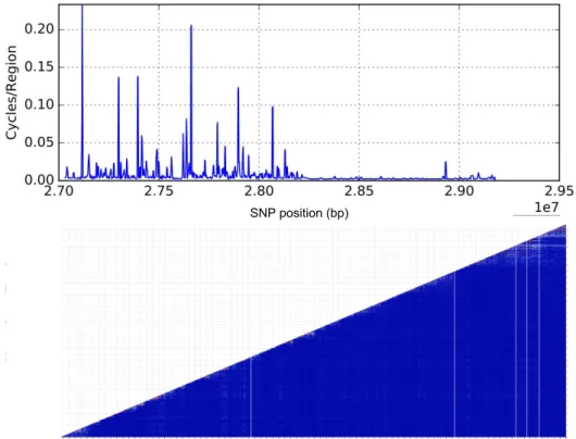
Figure 15 Linkage map and heatmap for chromosome 22 on a region between

2.70x107 _{bp to 2.95x10}7_{bp. 36}

Figure 16 Linkage map and heatmap for chromosome 22 on a region between

3.80x107 _{bp to 4.05x10}7_{bp. 37}

Figure 17 Linkage map and heatmap for chromosome 22 on a region between

4x107_{bp to 4.25x10}7_{bp. 38}

Figure 18 Simulation for 2 hotspots. 39

Figure 19 Simulation for 1 small platform. 40

Figure 20 Simulation for a platform with double the length of figure 19. 40

List of Figures viii

Figure 21 Simulation for 2 hotspots. 41

Figure 22 Simulation for 2 hotspots. 42

Figure 23 Simulation for 2 hotspots. 42

Figure 24 Linkage map for the X chromosome of male individuals with 30 SNPs (blue) and 20 SNPs (red), overlapping by 15 and 10,

respec-tively. 44

Figure 25 Linkage map for the X chromosome of female individuals with 30 SNPs (blue) and 20 SNPs (red), overlapping by 15 and 10,

respec-tively. 45

Figure 26 time-depth. 47

Figure 27 Linkage map for AFR (blue) and EUR (red) with the SNP that has a direct influence on the LCT gene (green). 49 Figure 28 Linkage map for AFR (blue) and EUR (red) with the SNP that has a direct influence on the LCT gene. Only individuals with the ancestral

allele (G) (green). 50

Figure 29 Linkage map for AFR (blue) and EUR (red) with the SNP that has a direct influence on the LCT gene. Only individuals with the alternate

allele (A; beneficial) (green). 51

Figure 30 Linkage map for AFR (blue) and EUR (red) with the SNP that has a direct influence on the HBB gene (green). 52 Figure 31 Linkage map for AFR (blue) and EUR (red) with the SNP that has a direct influence on the HBB gene. Only individuals with the

ances-tral allele (T) (green). 53

Figure 32 Linkage map for AFR (blue) with the SNP that has a direct influ-ence on the HBB gene. Only individuals with the alternate allele (A)

(green). 54

Figure 33 Linkage map for AFR (blue) and EUR (red) with rs2075984 (green). 55 Figure 34 Linkage map for AFR (blue) and EUR (red). Only individuals with

the alternate allele (green), for the rs2075984 SNP. 55 Figure 35 Linkage map for AFR (blue) and EUR (red). Only individuals with the ancestral allele (green), for the rs2075984 SNP. 56 Figure 36 Plot showing the starlikeness through the region with the SNP that has a direct influence on the LCT gene (green). 57 Figure 37 Plot showing the starlikeness through the region with the SNP that has a direct influence on the HBB gene (green). 57 Figure 38 Plot showing the starlikeness through chromosome 22 for 20 and 30

List of Figures ix Figure 39 Phylogenetic network outputted from the Network software GUI.

L I S T O F TA B L E S

Table 1 Populations present on the 1000 Genomes Project, their Code and number of samples. Information retrieved from the 1000genomes

web page 10

Table 2 Populations on the ExAC data, their code and number of samples. Information retrieved from the ExAC web page 11 Table 3 Populations on the ESP data, their code and number of samples. Information retrieved from the EVS web page 11 Table 4 Results for the number of cycles in each super-population 46 Table 5 Number of cycles present on a population that are on another

popu-lation, without duplicates. 46

Table 6 Results for the number of cycles in each super-population 47

L I S T O F L I S T I N G S

B.1 Python function cycle_numpy . . . 72 B.2 Python function to retrieve the information of only the neighbors of the center

node (root) . . . 73 B.3 Python function to parse the out file . . . 74 B.4 Python function to build a weighted graph object using NetworkX . . . 75 B.5 Python function to find the path where the starlikeness calculation will course 76

L I S T O F A B B R E V I AT I O N S

1000genomes 1000 Genomes Project. AF Allele frequency.

cM centiMorgan.

CNV Copy-number variation. DNA Deoxyribonucleic acid. DNA-seq DNA sequencing.

ESP Exome Sequencing Project. EVS Exome Variant Server.

ExAC Exome Aggregation Consortium. FTP File transfer protocol.

GUI Graphical user interface.

GWAS Genome-wide association study. HBB Hemoglobin subunit beta gene.

HbS Hemoglobin S.

LCT Lactase gene.

LD Linkage disequilibrium. LP Lactase persistence.

LPH Lactase-phlorizin hydrolase. MRCA Most recent common ancestor. mtDNA Mitochondrial DNA.

List of Abbreviations xiii

NGS Next-generation sequencing. PAR Pseudoautosomal region. ped Pedigree file format. rdf Roehl data format.

SFS CODE Selection on Finite Sites under COmplex Demo-graphic Events.

SNP Single nucleotide polymorphism. tbi Indexed tab-delimited file. VCF Variant Call Format. VDE VCFDataExporter.

1

DNA (deoxyribonucleic acid) molecules are composed by four nucleotides (bases): Ade-nine (A), Thymine (T), Cytosine (C) and GuaAde-nine (G). In Eukaryotic organism, including animals, DNA is organized into chromosomes and most are diploid at the somatic level, meaning that with the exception of the germ line (the egg and sperm cells) all cells pos-sess two copies of a given chromosome inherited respectively from the maternal and the paternal line of descent. The human genome contains 23 chromosome pairs, totaling 46 chromosomes from which 22 pairs are autosomes and a single pair, the X and Y sex chro-mosomes, which are different in females (two X chromosomes) and males (one X and one Y chromosome). Haploid cells in the germ line have only one chromosome from each pair and during the fecundation, a diploid egg is formed [4].

Although the genome of two unrelated individuals is almost 100% similar, a small set of differences (0.5%) is observable. These differences are responsible for many phenotypic differences between individuals but most are likely to be silent differences only observed at the DNA sequence level. This dissimilarity is explained due to sequence variations, which includes small insertions and deletions (indels) of one or more nucleotides, specific nucleotide substitution, which are the more common genetic variation, known as single-nucleotide polymorphism (SNP) [5], and copy-number variation (CNV), when abnormal copies of a chromosomal sections arise due to deletions and duplications (structural vari-ants) [6]. New mutations that arise through time may increase or decrease the risk to have a certain disease, yet the majority of them are likely to have a minimal impact.

When there is a SNP present on a sequence, both alternative nucleotides are denomi-nated alleles. The position with the variation is called a locus (and loci for various variable positions). Given this, the combination of several alleles within the loci of a region within a chromosome is called a haplotype. For instance, consider two SNPs from a region with six known SNPs (Figure 1); the former has alleles A and C; the latter has alleles T and G. The four possible haplotypes considering these two SNPs are AT, AG, CT and CG; however, only AT and CG are common [1].

1.1. Linkage disequilibrium 2

Figure 1.: Two common haplotypes from six SNPs. Retrieved from [1]

Considering that in diploid organisms (like humans) two copies of each chromosome exist in each individual it is not direct to extract haplotypic information. Seeing the case above one individual with the two most common alleles would appear as A/C in the third locus and G/T without a researcher knowing if the haplotypes were A-G and C-T or A-T and G-C. Although it is difficult to know individually haplotypes, on a grand scale of pop-ulation units it is possible to statistically estimate what are the most probable haplotypes, in a process called phasing [7].

When present in the exome (in the protein-coding regions) SNPs may be classified as two types, nonsynonymous and synonymous. A change in the DNA alters the codon (set of three nucleotides that code for a given amino-acid). Nonsynonymous SNPs encode dif-ferent amino acids due to the codon change, forming a difdif-ferent protein product. On the other hand, synonymous SNPs encode the same amino acid, and thus protein product, de-spite the allele difference (since different codons can code for the same amino-acid) [5].

1.1 linkage disequilibrium

Recombination rate is an essential parameter for most studies on human variation. Link-age disequilibrium (LD) is the association between two or more alleles that are more likely to occur simultaneously at different loci on the same chromosome, meaning that some specific haplotypes are more common than expected from the frequency of the individual alleles. When a new variant arises by mutation in a germinal line, that variant will be in complete linkage with the variants in the chromosomic background (or the alleles in the haplotype) where it arises. This mutation is passed into descendants if the mutant sex cell takes part in fertilization (germinal line) [8], becoming part of the population gene pool. If no recombination occurs the variant would maintain the chromosomic background where

1.1. Linkage disequilibrium 3 it initially emerged and the variant would be in complete LD with the variants in that back-ground. But recombination through time (occurring during meiosis due to crossing-over events between homologous chromosomes) will decrease the association between alleles, decreasing the LD in this process. Nevertheless, recombination events occurring during meiosis in each generation in a population has a cumulative effect on patterns of LD, de-spite being relatively rare over small regions and negligible on a small temporal scale [9]. Furthermore, patterns of LD are powerful tools in leading to the identification of demo-graphic events such as bottlenecks1_{, admixture}2 _{and population growth [10] and to the}

identification of events of positive selection [11]. For instance, in case of admixture be-tween two populations taking place, the descendant might have distinct segments within his genome inherited from different set of ancestors, possessing different genetic ancestries, which can be assessed through LD analysis [12]. Positive selection increases the frequency of a beneficial allele in a population. Reducing genetic variation on the region with the fixed advantageous variant on that population. This effect is known as the hitch-hiking effect, be-cause it increases the frequency of an allele that is in LD with the allele under selection [13].

1.1.1 LD measurements

Several ways to measure LD were proposed. The two most commonly used are D0 _{and r}2 (sometimes denoted₄2_{), both related to the coefficient of LD (D) that is given by (1) [14]:}

D= pAB pApB (1)

The frequency for allele A and for allele B are denoted by pA and pB, respectively. The haplotype frequency, considering allele A and B is denoted by pAB.

The first measure was proposed by Lewontin [15] for the normalized measure of D (D0_), where Dmax is the smaller value of pA(1 pB)and pB(1 pA), meaning the higher possi-ble value of D given the allele frequencies:

D0 ₌ D

Dmax (2)

1 A temporary reduction in population size that causes the loss of genetic variation. 2 The mixture of two or more genetically distinct populations.

1.1. Linkage disequilibrium 4

The second proposed measure is Pearson’s squared correlation coefficient (r2_{) [16] and it} represents other way to quantify LD:

r2= D2

pA(1 pA)pB(1 pB) (3)

Both measurements ((2) and (3)) are ranged between 1 (strong LD) and 0 (weak LD). If|D0_| equals to 1, two or three haplotypes are present; if it is significantly less than 1, all four haplotypes are present indicating recombination events. In case of r2_{being equal to 1, only} two haplotypes are present [10]. While the interpretation for maximum LD (1) and no LD (0) is direct, any value in between is difficult to interpret in terms of how strong LD is, as the values of_|D0_{|and r}2_{are highly dependent on allele frequencies and measurements are} not directly compared.

1.1.2 Patterns of LD

Although LD patterns are difficult to predict, there are regions in the human genome with weak evidence of historical recombination (strong LD) composing a model known as hap-lotype blocks (haploblocks) [17]. In addition, this model suggests the hypothesis to the existence of sites where much of the recombination occurs (hotspots). Furthermore, some studies were made to examine this theory and concluding on a ubiquitous existence of hotspots within the human genome [18]. However, the human sex chromosomes in males do not recombine in the same manner as autosomes or female sex chromosomes, but they have two homologous regions in which the recombination occurs in a similar fashion as the remaining 22 chromosome pairs. These short regions are called pseudoautosomal regions (PAR1 and PAR2); the first is the longest and has a physical length of 2.6 Mbp (2.6 mega base pairs; 2.6x106 _{bp) located at the short arms’ tips of X and Y chromosomes; the latter,} the PAR2, has a physical length of 0.32 Mbp and it is located at the long arms’ tips [19]. PAR1 exhibits in males a much higher recombination rate than PAR2 or the genome aver-age. PAR1 plays a key role in spermatogenesis and diseases [20,21].

The traditional method to map recombination rates, and thus hotspots, is to compare the physical map to the genetic map. Physical distance is the number of base pairs that separates two loci which is obtained by genomic sequencing, while genetic distance is cal-culated through recombination frequencies and indirectly by linkage. On that note, the

1.1. Linkage disequilibrium 5 measure for genetic distances is the centiMorgan (cM), defined by having a 1% chance of crossover between two genes on the chromosome. The average frequency of recombination in humans is 1cM per 1Mbp. Some regions near telomeres have generally much higher recombination frequency for both sexes, being higher in males [22], opposed to the low recombination (coldspots) found near the centromere for males, suggesting that recombina-tion rate in general is higher near the tips of the chromosomes.

1.1.3 LD observed in populations

Shorter haploblocks, and thus generally less LD and more divergent patterns of LD3 _were

observed on African populations that also display greater levels of diversity than non-African populations, probably suggesting an origin of modern humans in Africa (Figure 2) and a longer time for the disruption of LD patterns. Due to the Out of Africa movement migration of anatomically modern humans between 70 and 60 thousand years ago [23], that caused a bottleneck on the overall variation, the number and diversity of haplotypes is reduced when compared with Africa. This bottleneck consequently, increased severely LD on non-African populations [10,24,25].

As mentioned before, Africa is thought to be the ancestral homeland of modern hu-mans. Genetic studies on African human populations provide important information about how genetic variations alter the phenotype and for fine-scale mapping of complex diseases [26, 27]. Moreover, complex diseases like hypertension, diabetes, obesity and prostate can-cer are progressively present in African populations, presumably as a result to and urban-ized Western lifestyle. The possibility of existing population-specific alleles that predispose to disease, is very alluring for mapping these particular variants [28].

1.1. Linkage disequilibrium 6

Figure 2.: Humans Out-of-Africa movement in thousand years. [2]

1.1.4 Genome-wide association study (GWAS)

Understanding how recombination occurs throughout the genome is the basis to interpret various association studies (search from causal genetic variants for a given disease) and characterization of selective events. Likewise, genome-wide association study (GWAS) is a research approach that seeks to [29]:

• Detect variants associated with complex traits in populations, offering suspect re-gions;

• Study patterns of LD between SNPs to map genomic loci that have an effect on ill-nesses or other complex traits;

• Detect genetically causality for common complex diseases such as heart disease, dia-betes, auto-immune diseases and psychiatric disorder.

This type of studies will allow the identification of genetic markers associated with cer-tain diseases, making a statistical estimation for the increased risk of developing the dis-order. In some occasions, some variants are imputed, which means that genotypes are estimated for SNPs from the known LD patterns and haplotypes, using reference data. On that note, samples with shared haplotypes are used to estimate their frequencies among the genotyped SNPs. Association mapping studies look for LD between alleles that cause her-itable diseases and other nearby alleles, even though only a few may affect the phenotype [30,31].

1.1. Linkage disequilibrium 7 1.1.5 Positive selection

Positive selection increases the frequency of a beneficial allele in a population. Selective sweep takes place when genetic variation on the region is reduced caused by positive selec-tion. This is because the fixed advantageous variant on that population increased dramati-cally in frequency, and as its frequency increases at a fast rate, recombination was not able to break down the haplotypic background where the beneficial variant arose increasing the frequency of the complete haplotype, decreasing the overall haplotypic diversity [32]. This effect is known as the hitch-hiking effect, because it increases the frequency of an allele that is in LD with the allele under selection [33]. This process is the basis for selection tests, more exactly haplotype-based tests, that will measure the haplotypic diversity in one allele, in the allele under selection and the other allele. Such tests include the integrated haplotype score (iHS) [34] and the cross population extended haplotype homozygosity (XP-EHH) [35]. Addressing two regions to be explored later on that are an example of positive selec-tion that took place recently due to the presence of a new favorable allele. The lactase gene (LCT) and the hemoglobin subunit beta gene (HBB) are responsible for the ability to digest milk (lactase persistence) and resistance to some forms of malaria, respectively.

Lactase persistence (LP) is mostly common on European populations and less common on Africans. It allows the synthesis of the lactase-phlorizin hydrolase (LPH) enzyme to di-gest the lactose present on milk and other dairy products after weaning, possibly owing to positive selection [36, 37]. Although the SNP that will be studied is from the MCM6 gene, it has a direct influence on the LCT gene that encodes LPH. For the European population the rs4988235 is strongly associated with LP, specifically the LCT-13910*T allele. The poly-morphism is characterized by a C/T transition, where the individuals that have the T allele will carry the lactase persistence genetic trait [36,37,38].

The rs334 SNP located in the HBB gene, has an hemoglobin S (HbS) responsible for sickle-cell anaemia only on homozygote individuals (T;T). Despite having a strong dele-terious effect in heterozygous individuals (A;T), its presence provides a strong protective effect against malaria infection. This mutation is characterized by an A/T transition and is highly present on African populations, due to being a region with high prevalence of Malaria [39,40,41,42].

1.2. Variant Databases 8 1.2 variant databases

To discover sequence variations, next-generation sequencing (NGS) technologies were a breakthrough on DNA sequencing (DNA-seq). While the first human genome draft was accomplished during a period of nearly a decade and a half (using traditional Sanger se-quencing) [43] nowadays next-generation sequencing is allowing genomic and exomic data to be generated at an unprecedented level. As one example recently in a single Nature journal issues, hundreds of genomic sequences were published and analyzed [44,45,46].

Several databases focus on storing variation obtained from these genomes. In order to obtain a list of variants in a relatively user-friendly format the data needs to be processed using algorithms that will transform the data from raw data, that consists of millions of individual reads into, for example, a Variant Call Format (VCF) file, that will be widely used throughout this work.

An example of a pipeline from raw data to VCF files will be provided, focusing specifi-cally on the Illumina4_{DNA-seq pipeline chosen by the phase 3 of the 1000 Genomes Project}

(1000genomes). This type of sequencing produces reads (raw data) that are more commonly stored in FASTQ files along with the quality scores. Quality diagnostics are performed on the raw data to determine if preprocessing is necessary. The next step is to align/map the reads to a reference genome resulting in a SAM (Sequence Alignment/Map) file format or BAM (binary version). The Burrows-Wheeler Aligner (BWA5_{) is used for short reads}

mapping to the large reference human genome. Moreover, a post alignment preprocessing to remove bias is done before the final step of variant calling with an estimate on allele frequency (AF) and storage in a VCF file [47,48,49,50]. This will provide genotypes of an individual. However, the 1000genomes currently provides VCF files with haplotypic data (meaning that the data is in the so-called phase). This is obtained by a statistical method that uses complex algorithms to estimate the most probable combination of alleles given the population patterns. Such phasing is performed in the case of the 1000genomes with the software SHAPEIT2 [51,52], that performs this task on the full chromosome level. Furthermore, we will describe some databases of interest that, although all results focus on the 1000genomes, were used experimentally in the development of the work.

4 http://www.illumina.com/

1.2. Variant Databases 9 1.2.1 1000 Genomes Project

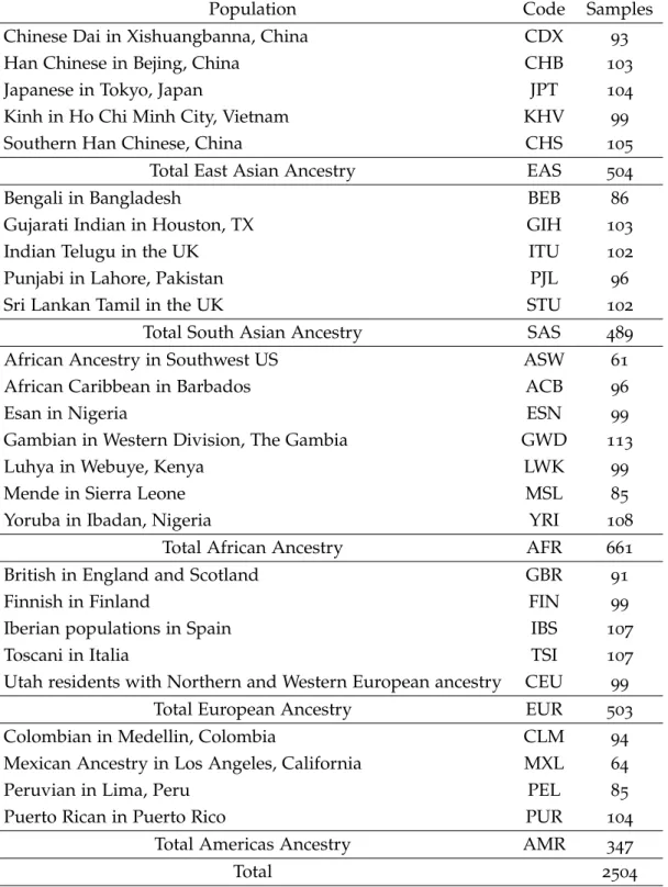
The 1000 Genomes Project (1000genomes) purpose is to catalogue variations present in the human genome from different genomics regions across 26 populations categorized in 5 super-populations, shown on Table 1 (with ancestry from Europe, East Asia, South Asia, West Africa and Americas).The objective is to characterize, using high-throughput sequenc-ing technologies, over 95% of variants with an AF of at least 1% and alleles present in coding regions with a frequency as low as 0.1% [53]. This dataset contains 78 million SNPs and was aligned using the GRCh37 reference genome assembly.

Throughout the 1000genomes, new variants were discovered and characterized, being added to the public database of short genetic variations (dbSNP6_{) or to the database of}

genomic structural variation (dbVar7_).

Due to the advance of sequencing technologies it is now possible to sequence genomes with a lesser cost. This NGS data provides a resource on human genetic variation. Each dataset may have different assembly algorithms and different coverage [54,55]. Genotyping these variants will reveal the alleles at particular sites or regions. All genotyped variants present in the 1000genomes data are phased, denoting the putative chromosome of the pair where that specific allele belongs. Most of the project contains low coverage data from pop-ulations suggesting that the individuals’ DNA was sequenced approximately 4 times (4x). This dataset contains samples from 2504 individuals, 1233 males and 1271 females.

Furthermore, the project allows to document the genotype profiles of the 2504 individuals from the last phase, phase 3, of the 1000genomes for further study, being accessible through a public FTP (File Transfer Protocol) server in compressed files (GNU Zip extension, ‘.gz’) [56]. Therefore, the fact that it is in a FTP server8 _{means that it is possible to download,}

upload, delete, rename or change permissions of files however one cannot access the files’ content remotely.

6 https://www.ncbi.nlm.nih.gov/projects/SNP/ 7 https://www.ncbi.nlm.nih.gov/dbvar

1.2. Variant Databases 10

Table 1.: Populations present on the 1000 Genomes Project, their Code and number of samples. Information retrieved from the 1000genomes web page

Population Code Samples

Chinese Dai in Xishuangbanna, China CDX 93

Han Chinese in Bejing, China CHB 103

Japanese in Tokyo, Japan JPT 104

Kinh in Ho Chi Minh City, Vietnam KHV 99

Southern Han Chinese, China CHS 105

Total East Asian Ancestry EAS 504

Bengali in Bangladesh BEB 86

Gujarati Indian in Houston, TX GIH 103

Indian Telugu in the UK ITU 102

Punjabi in Lahore, Pakistan PJL 96

Sri Lankan Tamil in the UK STU 102

Total South Asian Ancestry SAS 489

African Ancestry in Southwest US ASW 61

African Caribbean in Barbados ACB 96

Esan in Nigeria ESN 99

Gambian in Western Division, The Gambia GWD 113

Luhya in Webuye, Kenya LWK 99

Mende in Sierra Leone MSL 85

Yoruba in Ibadan, Nigeria YRI 108

Total African Ancestry AFR 661

British in England and Scotland GBR 91

Finnish in Finland FIN 99

Iberian populations in Spain IBS 107

Toscani in Italia TSI 107

Utah residents with Northern and Western European ancestry CEU 99

Total European Ancestry EUR 503

Colombian in Medellin, Colombia CLM 94

Mexican Ancestry in Los Angeles, California MXL 64

Peruvian in Lima, Peru PEL 85

Puerto Rican in Puerto Rico PUR 104

Total Americas Ancestry AMR 347

1.2. Variant Databases 11 1.2.2 Exome Aggregation Consortium

The Exome Aggregation Consortium (ExAC) is an affiliation of investigators with the ob-jective to compile exome (protein-coding regions) sequencing data from different projects that range from disease-specific individuals to population-specific datasets. The dataset is composed by 60706 samples, some representing individuals with severe diseases, of unre-lated individuals from 7 different populations (Table2). This merging of variant data from different projects will provide a base for the discovery of disease-causing variants [57].

Table 2.: Populations on the ExAC data, their code and number of samples. Information retrieved from the ExAC web page

Population Code Samples African/African American AFR 5203

Latino AMR 5789

East Asian EAS 4327

Finnish FIN 3307

Non-Finnish European NFE 33370

South Asian SAS 8256

Other OTH 454

Total 60706

1.2.3 Exome Sequencing Project

The National Heart, Lung, and Blood Institute created the Exome Sequencing Project (ESP) with the intent of sequencing the exome of richly-phenotypes populations, achieving 6503 samples from two different ancestries (Table3). Apart from a compressed dataset publicly accessible, this project has, a web interface known as the Exome Variant Server (EVS) that allows the visualization and extraction of filtered data to text files and Variant Call Format files. The ESP contains a mean coverage data of 81x [58].

Table 3.: Populations on the ESP data, their code and number of samples. Information retrieved from the EVS web page

Population Code Samples African-Americans AA 2203 European-Americans EA 4300

1.3. Relevant File Formats 12 1.2.4 Simons Genome Diversity Project Dataset

This database aims to include a list of genomes that were sequenced with a coverage of at least 30x using Illumina technology [45]. The database aims to display a wide range of anthropological and cultural diversity in terms of individuals.

This newly developed database offers an ideal dataset for the work described here, how-ever, it only provides the dataset in an unfriendly format for download (10 terabytes of data) and requires a certificate. The download is through a software that allows fast and se-cure (via encryption) data movement. The certificate needs to be approved and is required for security reasons (privacy of the files), when accessing the FTP channel to download the data [59].

1.3 relevant file formats

There are several file formats used in genomics and their features and levels of details incorporated are direct consequences of their use in different software.

1.3.1 Variant Call Format

To store variants, plus annotations, a file format was proposed by the 1000genomes, the Variant Call Format (VCF) file. Its adaptability and flexibility led to an increasing endorse-ment of the VCF file. On a similar note, VCF files were established as standard files to store DNA polymorphism data, such as SNPs, insertions, deletions and structural variants, including rich annotations.

1.3. Relevant File Formats 13

Figure 3.: VCF file format example. Retrieved directly from [3]

At the top, the VCF file contains several meta-information lines, each starting with ‘##’. These lines describe the data stored, which includes the type of variable associated with that data (integer, string, float, etc) and customized relevant information about the dataset. Below meta-information lines the actual genomic data will be displayed, starting with ‘#’, featuring 8 mandatory columns with specific fields, TAB-delimited. Particularly, this in-formation includes the chromosome column (CHROM), the start position of the variant according to the reference sequence (POS), unique identifiers of the variant (ID), the ref-erence allele (REF), the list of alternate alleles (ALT), quality score (QUAL), site filtering information (FILTER) and a list of additional annotation (INFO). Note that if samples are present in the file, sample columns will be added (sample ID) and a column regarding the information contained in the sample column (FORMAT). Genotypes separated by ‘|’ indicate the alleles are phased, if they are separated by ‘/’ they are unphased alleles [3]. 1.3.2 Input File Formats

The pedigree (ped) and map file formats are complementing type of files that are the most commonly used type of format in GWASs and they can be implemented using the software PLINK [60]. The ped file contains pedigree information and genotype calls and the map file contains variant information to complement ped file regarding the genomic position of the variants.

Some software tools use small variations in the file format in relation to PLINK. Such an example is the Haploview software that uses the ped file in combination with a file with extension info (similar to map) that provides information on the location of the SNPs along the chromosome. Haploview calculates LD patterns within a region [61] which it will be

1.3. Relevant File Formats 14 essential as a comparative tool in this work.

The Roehl data format (rdf) files are used by the Network software using a reduced median algorithm [62]. For the purpose of performing phylogenetics on the 1000genomes data the implementation of a software that builds networks makes more sense than into one that reconstruct straightforward trees, considering that the data can be shuffled by the so-called recombination between chromosomes.

The nexus (nex) file format is one of the most widely used formats in genetics. At its most simple form it includes the DNA data and the name of the individual samples but it can also include discriminated subsets.

The fasta file is considered the most basic DNA and protein sequence file format. It ba-sically contains only information of the sample and the sequence (in nucleotides or amino-acids) for a given region in text format.

2

2.1 relevant software 2.1.1 VCFDataExporter

The VCFDataExporter1 _{(VDE) is a tool mostly developed over last year using Python}

func-tions simultaneously with PyVCF that allowed the extraction of genomic data from the 1000genomes VCF files and transformation of that data into various formats useful in ex-isting genetic analysis software, mentioned before. The tool is now on his second release after further developments on the context of this project (v0.1.1) and provides the extrac-tion of genomic data from the 1000genomes dataset, ExAC dataset, ESP dataset and a user uploaded VCF file. From the user specified information imputed it is possible to extract the data and transform it into map, rdf, fasta, nex, ped, info, VCF and excel files, and generate some basic statistic regarding the data. After the requested files are created it will provide links for download or pop-up.

The conversion tool developed allows a user-friendly manipulation for researchers not used to deal with the large datasets established by NGS. On that note, a GUI on the form of a web app was developed using a Python web framework, known as Django. For a faster extraction of the region and his information a tab-delimited files indexer2 _{(Tabix) is being}

used to subset the VCF gzipped file with the completing indexed tab-delimited file (tbi). The subsetted VCF file will allow a faster retrieval of the genomic data and subsequent storage on different files.

2.1.2 Network Software

This software builds phylogenetic networks and trees, using several algorithms over a graphical user interface (GUI). It constructs a network following a multiple alignment of

1 https://github.com/raqsilva/VcfDataExporter

2 http://sourceforge.net/projects/samtools/files/tabix/

2.1. Relevant Software 16 sequences, in which each sequence is represented by a node and the edges, that connect one node to the other, represents the difference between each other (variants). This difference is seen if they differ exactly in one mutation. The network is constructed using the reduced median algorithm [62]. This algorithm consists on median networks which are composed by nodes connected by edges if there is a mutation between them. This type of method only accepts binary sequences. The median sequence results from the median binary val-ues of three sequences and is used to connect the nodes culminating on an unrooted and undirected phylogenetic network (Figure4). The median node could also be an existing se-quence if it corresponds to the median of the three other sese-quences. Median networks are mainly employed in the visualization of possible evolutionary pathways. On that note, the network will probably have all maximum parsimony trees; in other words, it will possibly have trees with the minimum number of nucleotide mutations [63].

The Network software will generate an output file (out file) for each rdf file used to run the program and build the phylogenetic network. Out files contain information about the data in rdf files and of the phylogenetic network. In this work, a modified version of the software provided by the developer was used. This version allowed batch work on several files to be performed while the downloadable version only allowed a single file to be run.

Figure 4.: Three haplotypes (grey) and the median node (white)

2.1.3 Haploview

Allows the visualization, from a GUI, of haplotype patterns within a region, calculates LD statistics, population haplotype frequencies and haplotype association tests. The several pairwise measures of LD calculated will be used to create a graphical representation of the region. This representation uses the haploblock model, mentioned on the introduction, to partition the region into segments of strong LD [61].

2.2. Relevant Libraries 17 2.1.4 PLINK

Is a command line program that performs genome-wide association analyses from samples’ genotypes. It is one of the main used programs in human genomics as it is used to filter data and merge datasets to be used in other software. Some of the main characteristics are [64,60]:

• Data management: recoding, reordering, merging and extracting subsets of data; • Summary statistics: missing rates and allele frequencies;

• Basic association analysis; • Population stratification; • Genotypic association models; • Extracting SNPs of interest; • Stratification analysis;

• Association analysis, accounting for clusters. 2.2 relevant libraries

2.2.1 PyVCF

In order to parse and extract specific data from compressed VCF files, the programming language Python and an API called PyVCF3 _{(v0.6.7) are the main mechanisms [65]. There}

is no need to decompress the compressed files before parsing, because the package comes with that attribute. Due to this feature the compressed files are preferred over the decom-pressed VCF files, since they are faster to transmit over the internet due to their reduced size and require less space on the disk for storage, contrary to the decompressed VCF files that have huge sizes (meaning it will be very difficult to handle them). Each VCF file has several records depending on how many positions are represented. It will attempt to parse the content of each record based on the data types specified in the meta-information lines, specifically the ##INFO and ##FORMAT lines. On that note, it is possible to extract ge-nomic data from compressed VCF files and transform that data into various formats useful in existing genetic analysis software (map, rdf, fasta, nex, ped, info).

2.2. Relevant Libraries 18 2.2.2 NetworkX

In pursuance of building graphs and analyze their structure this Python library was used. In addition, NetworkX4 _{has several characteristics including the possibility to generate}

di-rected or undidi-rected graphs, apply algorithms and do measurements, draw networks and add information to the network, edges or nodes. Furthermore, it allows to store networks in different formats and improve the access speed to the network data. This characteristic is very valuable to process data from large networks, like our phylogenetic networks, in a considerable shorter time.

3

Herein, this project objective is to extract information from the VCF files corresponding to the 1000genomes and analyze LD along a chromosome. This will be done through windows of polymorphic diversity along a chromosome. This work will partially build upon VDE, that was further developed also during this project. Due to their abundance, their importance in genomic variation and their simplicity of treatment, most of the data to be extracted and transformed in this work will be primarily SNPs. The objective is to transform each window into a network whose cycles will be an indication of the possible occurrences of recombination events. Such approach provides two advantages over tradi-tional measures. The first is that cycles might be a direct estimation of recombination events and consequently of recombination rate. The second is that the measure is not dependent of frequencies of the alleles or haplotypes and the sample size.

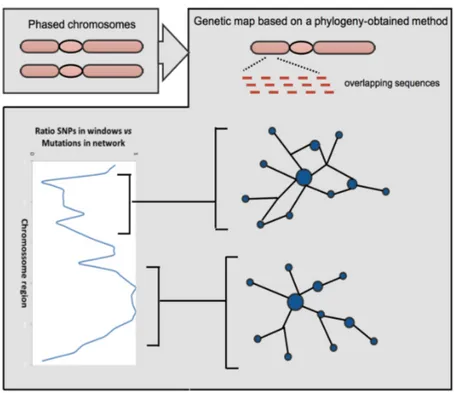
20

Figure 5.: Steps to build a recombination frequency map using a phyloge-netic based method

From the output of the network analysis, the main interest is in obtaining three measures: a) Number of mutations in the network. If there is no recombination (or multiple occur-rences of a given mutations which should be substantially rarer in autosomic DNA) in the segment the number of SNPs in the segment will match the number of mutations in the network. With recombination multiple mutations will appear in the network so ratio between number of mutations in the network and number of SNPs will provide a good relative measure for recombination frequency.

b) Each recombination event can generate a cycle (or reticulation) in the network. Count-ing the number of possible cycles in each generated network is a direct estimate for the recombination rate in the region.

c) Frequency increments (expansions) generate starlike figures in a phylogenetic context. In a genomic context an expansion within a given region of the genome might repre-sent a signal of positive selection. Phylogenetic starlikeness will be explored to see if it is a useful measure for selection evaluation.

Using measures in a) and b) a linkage map will be built. These linkage maps will be compared with maps based on traditional measures of linkage disequilibrium. VDE will be

21 directly used to create the complete chromosome files to be used in PLINK and Haploview. Additionally, in order to validate the approach, simulations will be used. A short evalua-tion of the potential of the use of recombinaevalua-tion detecevalua-tion will also be included.

Approaches for studying selection and the detection of selective sweeps will be employed, namely recombination maps comparing the two alleles (the beneficial allele and the other), based in well-documented cases of positive selection, but also across general chromosome maps based on the starlikeness measure.

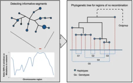
As a final analysis, if relatively long regions with no recombination are detected, network-s/trees of those longer stretches will be built, first using Network to make a final test for no recombination along the whole region.

Figure 6.: Steps to build a phylogenetic tree of long regions with no recom-bination

4

4.0.1 Data filtering

Through the analysis of existing VCF and rdf files, the comprehension and study of the structure of these files format was required. Parsing is done from a previously obtained VCF file, which contains the necessary data that will be used to create the rdf file with information to elaborate networks. First, it was considered multiallelic sites, however one decided that it was more accurate and straightforward to analyze only biallelic loci corre-sponding to binary data. To ensure that rdf files will only have polymorphic sites, SNPs are filtered by AF. In instances where analyses were based on groups with a continent-specific ancestry, the AF filtering for each population was performed based on the specific AF for the population and considering only samples belonging to that ancestry. Allele frequencies that are equal to 0 or 1 the SNP will not be included as it means that that locus is not polymorphic in that given population. Notwithstanding, this will allow the presence of at least the same number of mutations in the phylogenetic network as the number of SNPs in the rdf file.

Analyses were performed based on overlapping windows of 20 SNPs overlapping at 10 SNPs or 30 SNPs overlapping at 15 SNPs. Overlapping windows are acquired by con-sidering the first 20/30 SNPs, previously filtered, and then passing the last 10/15 SNPs to the next window adding 10/15 new SNPs, appending these. As a result, for each window 20/30 SNPs are present for each chromosome. To divide the information for each chromo-some each sample will be divided into two entries, corresponding to the two phased haplo-types, originating, for instance, HG00102a and HG00102b regarding the sample HG00102. However, concerning the case of the X chromosome in males there will be only one entry for each sample on sites that do not belong to PAR and two entries (a and b) on PAR. These regions were previously retrieved from the VCF file for future filtering by position, divid-ing chromosome X in three regions. The first region that corresponds to PAR1, the middle region and the last corresponding to PAR2.

23 Windows were successfully obtained extracting data along the VCF files with 20 or 30 SNPs overlapping by 10 or 15 SNPs, respectively, into various files. Output files are in rdf format for further use as input in the Network software and additionally a text informative file with the mutation number, SNP IDs and its genomic position was formed.

Each rdf file generated along a chromosome will be used to calculate a phylogenetic network, corresponding to the diversity in that window, and then produce an output file (out file) using the reduced median algorithm available in the Network software. The most effective way to use the algorithm for thousands of fragments was to contact the developers of the Network software, which were able to reprogram the software adding an additional feature capable of performing the algorithm on multiple files instead of requiring each file to be selected individually. This characteristic allowed to generate all the thousands of out files from all rdf files of windows along a from the chromosome.

Specific data from two interesting SNPs that have been firmly established as two ex-amples of positive selection in the human genome will be analyzed. The SNPs chosen are responsible for having a direct influence on the expression of the LCT gene (rs4988235) and HBB gene (rs334) that respectively allows the digestion of lactose and offers protection against Malaria. Moreover, a region surrounding the genes/SNPs of about 4 million base pairs is chosen from the VCF file of chromosome 11 to include the HBB gene and from the VCF file of chromosome 2 to include the SNP (located in MCM6 gene) that has influence on the LCT gene. Following this, these regions are outputted in a new VCF file for each gene. In the 1000genomes data the transition of rs4988235 and rs334 is characterized by G/A (in-stead of C/T like mentioned before) and T/A, respectively. For each gene, samples from EUR or AFR were the only ones considered, and the haplotypic data was separated into different folders based on the geography. Following this, the data was further separated based on the presence of the SNP or not in the haplotype, where one folder will contain an rdf file with the haplotypic information of the chromosomes that have the reference allele, and the other folder will contain the haplotypic information in the chromosome that have the alternate positively selected allele.

4.0.2 Data processing

Two files (out file and text informative file) are essential to extract required information on phylogenetic networks. To ensure these steps Python scripts were written, including the development of efficient methods to store, retrieve and process large amounts of data. The out file contains the necessary data to build a graph with NetworkX and count existing

24 mutations. This data consists in nodes and edges with the respective mutation number. Moreover, it was possible to count all cycles (reticulations) obtained from the connection of 4 nodes (1 being equal; first and last node) by 4 edges that have the same 2 mutations; and obtain the SNP IDs that are contained in those edges (FunctionB.1). The text file provides the SNP ID and the genomic position of each SNP, which allows calculating the region size by subtracting the genomic position of the last SNP with the first. This gathered infor-mation is used to build a plot for the visualization of the measurements of recombination frequency throughout the chromosome with matplotlib1_{. Recombination rate in the region}

is measured by the ratio between cycles and region size; while a second linkage measure was established by the ratio between mutations and region size. All the data was stored in a tab-delimited text file.

Figure 7.: Pipeline of the process to generate required data. Light gray are the output files and dark gray are software or scripts implemented during the workflow.

25 Cycles in populations

The output from the reticulations accounted for each population are important to explore the use of recombination as a clock, it will be explored assuming an African origin for Modern Humans and the Out-of-Africa movement. In this regard, all cycles from each of the five main population groups (Africa, Europe, South Asia, East Asia and America), along the different windows of chromosome 22, were calculated and they were compared with the cycles from the other 4 populations. For this to be possible, scripts were made elaborating an algorithm to course through the entire network from each window finding all reticulations (cycles) in the least time consuming way and considering the computing resources available. The algorithm (Function B.1) will course only through the nodes that are connected, owing to being those that aren’t leaf nodes and probably resolving into cycles. It will select a node (n1) coursing through all neighbors and saving the SNP ID (e1) linking it with the neighbor (n2) and edge, then checking all neighbors from n2 (namely node n3), not equal to n1, and saving the respective SNP ID (e2) of the edge. Then it will search for the neighbors of n3 and compare e1 with the SNP ID of the edge that connects n3 to the neighbor (n4). If the SNP IDs are equal it will continue the course if not, the algorithm will try other neighbors. This n4 node will have to be connected to n1 and have the same SNP ID as e2 to complete a cycle. All information related regarding edges and neighbors is stored. The SNP IDs that define each cycle are in a list ([e1, e3]) which will be stored in a text file. The forthcoming analysis between comparing matches in the cycles of each specific population against another simply corresponds to a search for a cycle in one population or its inverse ([e3, e1]) in the file of the other population.

Figure 8.: Cycle example.

Starlikeness

Using our phylogenetic network, we built a phylogenetic tree based on the most probable evolutionary path with the minimum number of evolutionary events established from the maximum parsimony method, eliminating edges that are part of the reticulations (cycles) [63,66]. The graph will have to be weighted for the calculation of a Dijkstra path from the

26 central node (root) to all other nodes present in the network. The central node is the node with higher degree, which is the node with more edges connected to it. Dijkstra algorithm will find the minimum cost path (optimal path) between all nodes in the graph [67]. In this case we will find the optimal path from the central node to all other nodes. The optimal path is found because all edges have a weight attribute that was implemented specially for the algorithm. The weight of each edge depends on the frequency of haplotypes on each node that compose the edge. Moreover, nodes without samples (like median vectors) are given an edge weight of 2 and all other nodes have an edge weight of 1 (Function B.4). Furthermore, Dijkstra paths are computed and phylogenetic trees are built based on those paths.

The tree root is considered the most recent common ancestor (MRCA) and the other existing nodes are related to this central node by mutations that occurred on specific sites connected by edges. Additionally, this tree demonstrates the mutational history. The coa-lescence time is the time that has elapsed since the presence of the MRCA of several copies of a locus [68,69]. Given each node with n haplotypes in a tree with i edges and that edge with m mutations, we estimated the variance (r2_{) of the coalescence time (r) that can be} calculated by [70]: r= S ni⇥mi ntotal (4) s2= S n 2 i ⇥mi n2 total (5) Where the theoretical value, which when equal to 1 corresponds to a perfect star phy-logeny, is given by [70]:

s_t2 = r

ntotal (6)

And the final calculation for the starlikeness of the network is:

starlikeness= st2

s2 (7)

After calculating the variance, the theoretical variance and the starlikeness for each over-lapping windows, a plot with those values was built to verify the starlikeness throughout

27 the chromosome.

4.0.3 Data simulation

Simulations were performed using SFS_CODE (Selection on Finite Sites under COmplex De-mographic Events), which is a software that generates population genetic simulations. It has the capacity to generate populations of individuals and follow them generation by gen-eration evolving by natural selection. Evolutionary algorithms are applied so that a given number of individuals hypothetically evolve under different levels of variation, selection and inheritance, including important recombination mechanisms like crossing-over and gene conversion (unidirectional transfer of genetic material) that can be modulated by the user. Demographic effects and migration can be included. Furthermore, DNA sequences are generated for each individual in the simulations and aligned. Due to the simulation of finite-sites mutations this alignment may contain several sites that could have being a target of several mutations (homoplasy) which could cause false possible recombination events [71,72,73]. Nevertheless this is also a strong possibility in real data which can allow the simulations to mimic false positives that we could find in real data.

All simulations using one chain of iterations were only performed in a population con-taining 1000 diploid individuals for a single locus of 50000 bp with a mutation rate of 0.01 per site. Outputs are given in VCF files. To analyze how the novel measure performed, sev-eral simulations were done on different regions with high/low recombination, like larger regions with a stable rate of recombination, regions with 2 different rates, small regions with high recombination (hotspots) to search for peaks and different peak sizes depend-ing on the recombination rate. SFS_CODE takes a recombination map file which employs crossing-over and gene conversion. This file contains the number of sequence intervals (re-gions with different recombination probability), the base pair position and its cumulative recombination probability until this site. Each simulation was performed three times with the same recombination map file.

4.0.4 LD heatmap

Haploview has a limitation of 100kbp (100 kilo base pairs; 100x103 _{bp) for the graphical} representation of the region. This limit can be overcome with higher computing resources and a specific command of haploview, but in this case the resources were far from sufficient. As a result, the visualization of haploblocks from the measures of LD was not possible

us-28 ing this software. A pipeline was developed to be able to visualize these LD patterns on larger regions. To subset large regions, like a substantial part of a chromosome, the use of bcftools2_{was needed in behalf of its fast subsetting and filtering command (view). This tool}

allows to subset the VCF file into smaller regions with a filtering option of keeping only the SNPs that have an AF higher than a threshold value. The subsetting will require the tbi file of the VCF file to retrieve the information faster. Then, vcftools3_{will get as input the VCF}

file originated from bcftools and output the Pearson’s squared correlation coefficient (r2_{) in} a tab-delimited file containing the chromosome, the SNPs positions of the two SNPs com-pared and the corresponding r2_{. With the outputted LD file, a Python script was written to} be able to read the file and extract the useful data. Additionally, the data is composed into a matrix and then with the resources of plotly4_{, a heatmap was built. The heatmap contains a}

color scheme, which the blue color represents lower values of r2 _{and red represents higher} values of r2_{. Seemingly, haploblocks are represented as triangular red regions.}

2 https://samtools.github.io/bcftools/ 3 http://vcftools.sourceforge.net/ 4 https://plot.ly/

5

All the plots shown are the mean of 14 values (windows) for the measures of Cycles/Region and Mutations/Region. From the original tab-delimited files all the values are retrieved with an overlap of 7 values. This was done so that a tendency across a given portion of the chromosome was obtained and so that individual single high values do not generate a dis-proportionate peak that could actually be caused by sequencing faults (as the 1000genomes data is low coverage data).

5.1 linkage maps from the study on chromosome 22

Chromosome 22 is the most recombinant chromosome on humans, having a recombination frequency of 2.46cM per Mbp against the genome average of 1cM per Mbp [74]. This is expected as it is the shortest chromosome, so if homologous chromosomes connect during meiosis at least in one point and crossing over occurs, the rate of recombination will be higher considering its size. Chromosome 22 due to its high recombination rate and the smallest size (for computational reasons) is a good model to test the new approach.

5.1. Linkage maps from the study on chromosome 22 30

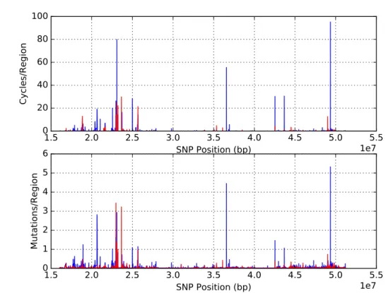
Figure 9.: Linkage map for chromosome 22 with 30 SNPs (blue) and 20 SNPs (red), overlapping by 15 and 10, respectively.

Figure 9 shows that independently of the measure employed (cycles or number of mu-tations divided by size) or the fact that measures are based on 20 or 30 SNPs the maps are very similar. Also it becomes really explicit that along the chromosome it is possible to identify regions with low levels of reticulation in the region, likely meaning very low recom-bination, as well as regions displaying peaks that could represent recombination hotspots. Throughout the thesis the maps of these measures will be generally referred as ”linkage maps” although the first map could better represent a recombination rate map and the sec-ond, based on the excess of mutations in the phylogenetic reconstruction is more difficult to define.

It becomes really explicit that along the chromosome it is possible to identify regions with low levels of reticulation in the region, likely meaning very low recombination, as well as regions displaying peaks that could represent recombination hotspots. At least four or five regions with putatively high recombination rate are visible, corresponding to various peaks on the same general area (namely around the positions, in bp, 2.2⇥107 _{to 2.6⇥10}7 and just after 3.5_⇥107_).

5.1. Linkage maps from the study on chromosome 22 31

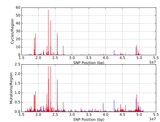
Figure 10.: Linkage map for chromosome 22 with 20 SNPs, overlapping by 10. African individuals (blue) and European individuals (red).

Figure 11.: Linkage map for chromosome 22 with 20 SNPs, overlapping by 10. Euro-pean individuals (blue) and South Asian individuals (red).

5.1. Linkage maps from the study on chromosome 22 32

Figure 12.: Linkage map for chromosome 22 with 20 SNPs, overlapping by 10. South Asian individuals (blue) and East Asian individuals (red).

5.1. Linkage maps from the study on chromosome 22 33

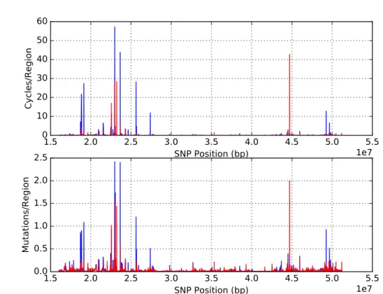
Figure 13.: Linkage map for chromosome 22 with 20 SNPs, overlapping by 10. East Asian individuals (blue) and American individuals (red).

Another relevant analysis is the comparison of maps between networks established on a single population. (Figures 10, 11, 12, 13). The objective is to observe if recombination maps varied drastically depending on the dataset, especially considering that one of the advantages of this methodology is that it should not be so dependent on allele frequencies. The maps did not vary significantly between population. For example, all graphics show a region between 20Mbp and 26Mbp (base region) that has a higher recombination frequency than other regions on the plot independently of the population analyzed (Figures10,11,12, 13).

A comparison between African (AFR) and European (EUR) populations shows that, as expected, observed recombination is larger in African populations (Figure 10). Although it is evident that the recombination rate on individuals with African ancestry on chromo-some 22 is higher than European individuals, being especially clear on the region 22Mbp and 26Mbp. The higher peak of recombination (hotspot) is almost 100 Cycles/Region for AFR and 30 Cycles/Region for EUR populations. This observation is in line with the fact that modern humans had an origin in Africa while outside Africa a bottleneck occurred when starting the populating of the globe that would partially increase the linkage.

5.2. Linkage maps compared to heatmaps 34

Apart from a few larger peaks, the recombination frequency is very similar between South Asian (SAS) populations and European populations (Figure 11). The difference be-tween SAS and East Asian (EAS) populations is narrow, which is expected considering that even though South Asia was settled before East Asia, it was likely a very rapid migration [75, 76] leaving little time for differentiation (Figure 12). The Americas were likely colo-nized by modern humans from a Northeast Asian source [76]. It is clear that apart from a few peaks, America has a lower base recombination rate than East Asia (Figure 13). With the course of time and space between the possible movement of humans from Africa to America, the observed recombination is thought to decrease which is caused by successive bottlenecks. Nevertheless, maps are not extremely different between populations.

5.2 linkage maps compared to heatmaps

In order to compare this new methodology with methodologies that have been established for a long time in genetics, like traditional linkage disequilibrium measures, a comparison of different regions will be established. It is impossible to compare the full chromosome for r2 _{since software tools like Haploview would just allow 100kbp, that is a very small} size in a chromosomal context. The pipeline developed here allowed to build LD maps for 20 times larger regions than haploview. The blue color represents lower values of r2 and red represents higher values of r2_{. Following we will compare different stretches of} chromosomic regions using the linkage map developed here and the heatmaps. For a simplistic descriptive statistic of the region, an average of the Cycles/Region and linkage measure for that portion will be presented. The examples aim to provide instances of agreement and disagreement between the two methodologies.

5.2. Linkage maps compared to heatmaps 35

SNP position (bp)

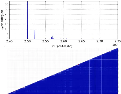
Figure 14.: Linkage map and heatmap for chromosome 22 on a region between 2.45x107

bp and 2.75x107_bp.

The mean Cycles/Region for the linkage map (Figure14) is 0.17. Comparatively, this is a region with relatively high recombination rate considering this measure. Analogously, the heatmap does not have any significant haploblocks, hypothetically due to the high recom-bination rate.

5.2. Linkage maps compared to heatmaps 36

SNP position (bp)

Figure 15.: Linkage map and heatmap for chromosome 22 on a region between 2.70x107

bp to 2.95x107_bp.

On figure 15 the mean recombination frequency based on cycles is approximately 10 times lower than the region displayed in figure 14, but there are not relevant haploblocks present. It could be explained by a not very accurate calculation of LD (using r2_{) or the} linkage map not being correct in that region (possibly due to a small number of SNP on the overlapping windows). This is the region that shows lower correlation between the results we obtained with r2 _{and the new methodology. It is not straightforward to explain and} deserves a detailed examination in the future in terms of frequency of the different alleles along the region, since a first analysis does not reveal anything particular.

5.2. Linkage maps compared to heatmaps 37

SNP position (bp)

Figure 16.: Linkage map and heatmap for chromosome 22 on a region between 3.80x107

bp to 4.05x107_bp.

The region displayed in plot 16 has an average recombination frequency of 0.046, yet this value is high due to a peak of approximately 14 Cycles/Region that is increasing the overall recombination rate. When observing the heatmap it is possible to see that some haploblocks are found, specially two stronger ones between 3.88 to 3.93 confirming the low recombination rate in the region. However, right after these blocks r2_{is low, corresponding} to the peak in the new methodology.