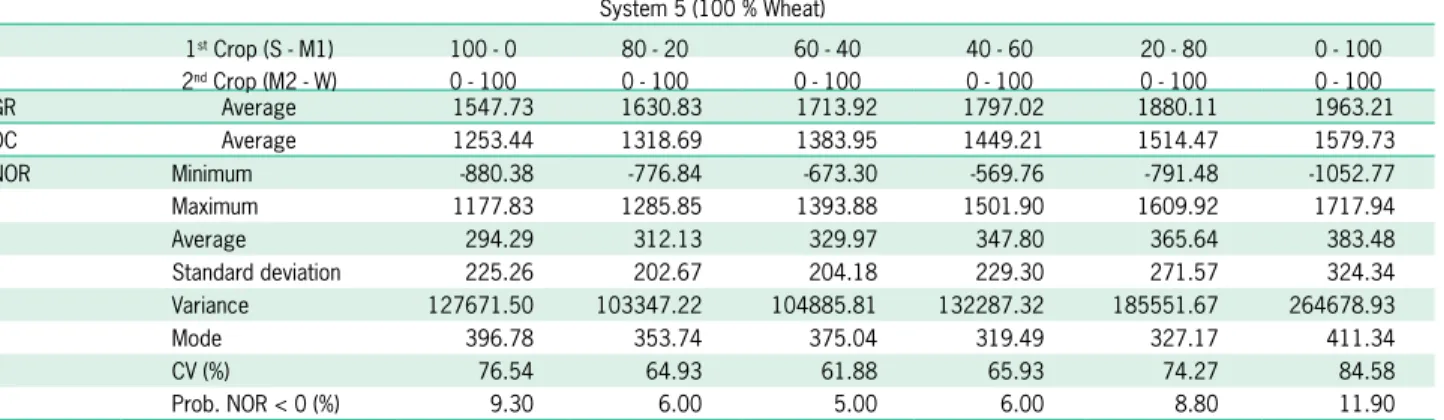
Risks associated with a double-cropping production system – a case study in southern
Texto
Imagem
Documentos relacionados
Observamos, nestes versos, a presença dos deuses do amor, Vênus e seu filho, o Amor ou Cupido, ligados aos vocábulos bella e rixae, guerra e disputa, ou seja, o amor é uma guerra
Peça de mão de alta rotação pneumática com sistema Push Button (botão para remoção de broca), podendo apresentar passagem dupla de ar e acoplamento para engate rápido
É importante destacar que as práticas de Gestão do Conhecimento (GC) precisam ser vistas pelos gestores como mecanismos para auxiliá-los a alcançar suas metas
Neste trabalho o objetivo central foi a ampliação e adequação do procedimento e programa computacional baseado no programa comercial MSC.PATRAN, para a geração automática de modelos
Ousasse apontar algumas hipóteses para a solução desse problema público a partir do exposto dos autores usados como base para fundamentação teórica, da análise dos dados
oral para opacificar o trato gastrointestinal está indicado para a detecção de tumores para aórticos no retroperitônio, devido ao fato de o intestino
Dentre essas variáveis destaca-se o “Arcabouço Jurídico-Adminis- trativo da Gestão Pública” que pode passar a exercer um nível de influência relevante em função de definir
The results showed that the higher effi ciency in light energy uptake, paired with better photochemical performance and better CO 2 fi xation in plants under direct sunlight
In ragione di queste evidenze, il BIM - come richiesto dalla disciplina comunitaria - consente di rispondere in maniera assolutamente adeguata alla necessità di innovazione dell’intera
