of Chemical
Engineering
www.scielo.br/bjcePrinted in BrazilVol. 35, No. 01, pp. 69 – 89, January – March, 2018
*Corresponding author: Camila P. Pereira. Email: [email protected] dx.doi.org/10.1590/0104-6632.20180351s20160370
DEVELOPMENT OF ECO-EFFICIENCY
COMPARISON INDEX THROUGH
ECO-INDICATORS FOR INDUSTRIAL APPLICATIONS
Camila P. Pereira
1,*, Diego M. Prata
1, Lizandro S. Santos
1and Luciane P. C. Monteiro
1 1 Departamento de Engenharia Química e de Petróleo,Universidade Federal Fluminense,Rua Passo da Pátria, 156 –D, 24210–240, São Domingos – Niterói, RJ 24210–240, Brazil. (Submitted: June 11, 2016; Revised: November 6, 2016; Accepted: November 13, 2016)
Abstract – In the last decades companies aligned with the concepts and principles of sustainable development have been seeking to minimize the environmental and social impacts caused by their operations. Typically, the primary environmental concerns in the industry were related to water consumption, wastewater production, waste generation, energy consumption and mainly CO2 emission - which is one of the causes of the greenhouse effect. However, the environmental eco-efficiency is not clearly seen when the evaluations of these eco-indicators are individually used and, therefore, it becomes necessary to implement a methodology that enables a joint assessment involving various aspects. In this paper we have developed an environmental index, called Eco-efficiency Comparison Index (ECI), applied to evaluate in real time a petrochemical facility. Throughout a study-case based on experimental data, the results have evidenced that the ECI is a useful tool for eco-efficiency analysis for process monitoring.
Keywords: eco-efficiency, eco-indicator, industrial facility.
INTRODUCTION
The rise in global warming, energy consumption and gas emissions has been the object of investigation of several studies. There are numerous methods and
indicators capable of describing environmental efficiency
or some of its components. The approaches and principles
of these practices and indicators vary due to differences in
industrial applications and desired outcome.
According to the World Business Council for
Sustainable Development (WBCSD), eco-efficiency is
competitive in production and marketing of goods or services that satisfy human needs, improving the quality of life, minimizing environmental impacts and intensity of natural resource use and can consider the entire life cycle
analysis (LCA) of production (WBCSD, 2000). Thus,
it allows achieving the social, ecological and economic
parameters, aiming to reduce the consumption of resources
(energy, water, materials, raw material, etc.). At the same time, eco-efficiency may minimize the impact on nature (water consumption, air emissions and dispersion of harmful substances) while maintaining and enhancing the value of the manufactured product (Maxine et al. 2006).
When addressing emissions and waste of a typical industry, such analysis is limited to only one of the
elements in the entire chain (from the production to the delivery of the service to the user). However, life cycle analysis (LCA) is a broader study because a more detailed
study can be made, showing a way of understanding the
impact of different alternatives (Jollands, 2003).
Environmental indicators that aim to measure the
were introduced into the literature by Tyteca (1996). The eco-indicators are defined as an environment variable (i.e., consumption) divided by an economic variable (i.e., production or production cost) (Maxine et al., 2006; Siitonen et al., 2010). However, another way to calculate an eco-indicator is using the reciprocal of this form (Tahara et al., 2005; Kharel and Chamondusit, 2008), often replacing production by monetary income (revenue) as the economic
variable.
Usually the eco-efficiency analysis is difficult when measurements are observed from a single eco-efficiency
indicator. Thus, it becomes necessary to evaluate a set of indicators to provide a complete evaluation of an industrial
process. However, it is worth emphasizing the difficulty
in benchmarking when the indicators are used together
(consumption of energy and water, wastewater and waste
generation and CO2 emission, for example). In this context,
the indicators may not be enough to evaluate efficiency if
they are presented separately. Given this, synthesize them as an index can be a useful solution.
Petrochemical plants are a relevant source of atmospheric emissions of carbon dioxide, carbon monoxide, methane, oxides of sulfur, oxides of nitrogen, etc. The petrochemical industry represents one of the most relevant industrial sectors in Brazil. Its production volume will tend to expand in the coming years with the
construction of new petrochemical plants (Rio de Janeiro - COMPERJ; and others states of Brazil like Ceará, Pernambuco and Maranhão). Usually, the activities of the petrochemical industry consume significant amounts of
energy and water and produce intrinsically CO2 emissions
to the atmosphere, as well as water wastes (effluents) and
solid wastes.
Based on the previous remarks, this work aims to develop a global method to compare, in real time, the
eco-efficiency of a petrochemical company. The goal is
to construct a monitoring tool capable of summarizing in
eco-efficiency indexes the main environmental aspects of
the operational conditions and their primary environmental impacts, including global warming, photochemical ozone
creation, soil acidification and human toxicity.
In the next section, the industrial applications of
eco-indicators are briefly reviewed, and the concepts
and methods for environmental construction tools are
discussed. In the Methodology, the Eco-efficiency
Comparison Index method is proposed. In sequence,
the industrial petrochemical plant is briefly introduced.
Subsequently, the results based on the process analysis are presented. Finally, we conclude the article, summarizing and suggesting remaining issues for future research.
LITERATURE REVIEW
Since some organizations began to be concerned about environmental issues, such as the realization of
“Our Common Future” in 1987 and “Agenda 21” (Rio de Janeiro, Brazil) in 1992, governments of many countries
and organizations have emphasized the importance of the concept of sustainability. Such concept includes the integration of the economic, social and ecological
pillars (Cote and Hall, 1995; Lowe and Evans, 1995; Charmondusit, 2009) and it allows fitting the needs of
the present generation without compromising the ability to meet the needs of future generations. Furthermore sustainability integrated into performance management systems brings concrete innovations in organizational culture and processes as it prioritizes resources, monitors current activities and presents results of pursuing agreed targets.
Some eco-indicators focus on simple function between environmental and economic variables, generally used
for industrial process monitoring; whereas other more
sophisticated tools enable the joint utilization a set of
eco-indicators (e.g., “Environmental Fingerprint” method) for analysis of different alternatives. Some of these tools are
overviewed in the following sections.
Efficiency measurement
A range of methods has been applied to measure
various efficiency concepts. Such strategies, therefore, can take many different forms according to the goal,
object or system analyzed, and the methodology taken by researchers or practitioners. It can involve the use of
Efficiency Indicators, Economic-Ecological Models,
Simulation Modeling, Decomposition Analysis, Computable Equilibrium Models, Input-Output Analysis, Ecological Multiplier Analysis, Multiattribute
Decision-making (MADM) and Complex Adaptive system Models (Jollands, 2003). Such methods are useful to measure efficiency in LCA; however, they can also be applied to measure eco-efficiency in a more restrictive way.
The Material Input per Unit of Service (MIPS) concept can be used to measure eco-efficiency of a process or
product. The method takes into account materials required to produce a product or service in which the material
input (MI) is divided by the number of service units (S) (Cahyandito, 2009).
According to Jollands (2003), Decomposition analysis
is a powerful tool that provides the analyst with the
ability to identify the key factors that effect eco-efficiency
indexes. Studies have pointed out that principal component
analysis (PCA) is a relatively accurate method, in that it
reduces the number of data dimensions without much loss
of information. However, such methods can suffer from rotational ambiguity, which means that different solutions may produce the same fit to the data matrix (Jollands, 2003).
with aggregate eco-efficiency indicators. According to the
author, FA/PCA is a promising method, in that it reduces the number of data dimensions without much loss of information.
Wu et al. (2012) applied a new variant of Factor Analysis, the so-called Positive Matrix Factorization (PMF) to the problem of weighting and integrating eco-efficiency
indicators. According to the authors, the results of PMF are guaranteed to be non-negative, while the results of FA often cannot be rotated to eliminate all negative entries.
In Woon and Lo (2006) a modified eco-efficiency indicator
was developed to integrate the life cycle human health impact associated with two proposed waste disposal facilities. The
modified index was based on a two-dimensional graph. The first dimension was calculated through the life cycle
costing and the second one by the life cycle human health
index. According to the authors, the modified eco-efficiency
indicator involving environmental and economic aspects of the proposed facilities from a life cycle perspective facilitates the stakeholders in developing policy guidelines for pursuing
an eco-efficient management.
Eco-indicators for eco-efficiency analysis
An eco-indicator is usually expressed in relative terms: a ratio between economic and environmental variables.
Based on the works of Sittonen et al. (2010), Zhou et al. (2010), Liu et al. (2011), Zhang et al. (2012) and
taking economic variables such as production, these
eco-indicators can be defined as:
y Water Consumption - Ratio of the total water consumed
in a period by the total production equivalent (m3 / t).
y Energy Consumption - Ratio of total energy (all energy
sources, including electricity) consumed in a period by the total production equivalent (GJ / t).
y CO2 Emissions - Ratio of total CO2 emissions
(combustion, indirect and fugitive) in a period by the total production equivalent (t / t).
y Wastewater Generation - Ratio of the total effluents
generated in a period by the total production equivalent
(m3 / t).
y Waste Generation - Ratio of the total solid waste generated in
a period by the total production equivalent (kg / t).
The information and experience from both the high administrative sectors and factory employees who deal directly with the process are essential to collect data that can provide valuable information for the development of eco-indicators. However, an eco-indicator should not be analyzed separately but aggregated with other eco-indicators. Such eco-indicators may form an environmental
index to evaluate the eco-efficiency. Thus, for a complete
evaluation, the development of an environmental index for
comparison of eco-efficiency is necessary.
In recent years researchers have found new ways to aggregate complex datasets including social-economical and environmental data. Proper selection of environmental indicators is the most important decision for the evaluation
of the eco-efficiency of the industry (Nordheim and Barrasso, 2007). According to Veleva and Ellenbecker (2001), the construction of indicators should be based on five criteria. (i) The determination of the unit of measurement for calculating the indicator; (ii) the type of measurement (absolute - measure a total amount - or relative); (iii) the period of analysis; (iv) the development of objectives and (v) the targets and limits (how much a company wants to measure the indicators covered).
Aggregate indexes are potentially useful for indicating complex information succinctly to decision makers. It is possible to construct a general mathematical framework that accommodates the many options for aggregating
eco-efficiency indicators instead of comparing directly input and
output data. Such calculation consists of two fundamental
steps: (i) calculation of the sub-indexes used in the final index; (ii) aggregation of the sub-indexes into the overall
index. The aggregation function can involve summation, multiplication and maximum or minimum mathematical operations. Examples of aggregate indexes are Ecological Footprint/Fingerprint, Index of Sustainable Economic
Welfare, Pollution Index, Unified Global Warming Index, etc. (Jollands, 2003). Their greatest contribution is the
simplicity and ease of understanding for the policymaker
unfamiliar with environmental issues (Ichimura, 2009). The weighting step of an eco-efficiency analysis
transforms and aggregates environmental inventory
data, which can be a significant number of different parameters, to a single index. Many different weighting methods are used in industry. The main differences can
be assigned to which reference for evaluation that is chosen, which principle is applied for the assessment and whose preferences the evaluation is based upon. Another important aspect is the spatial extension of the weighting method, i.e., for which geographic region the weighting
method is compatible with. Different weighting methods
have been used in industry: BASF, Eco-Indicator 99,
Ecopoints, Environmental Themes, etc (Borén, 2008). Eco-indicators for assessing eco-efficiency have been
reported in the literature for some applications in industry,
such as aluminum (Nordheim and Barrasso, 2007), iron (Kharel and Charmondusit, 2008), steel (Siitonen et al., 2010; Van Caneghem et al., 2010), iron and steel (Zhang et al., 2012), petrochemical (Charmondusit and Keartpanpraek, 2011), ammonia (Zhou et al., 2010), calcium (Liu, et al., 2011), cement (Von Bahr et al., 2003) and sugar cane (Ingaramo et al., 2009).
The most recent papers are described below:
Rattanapan et al. (2012) developed eco-efficiency
based on material flow analysis. The result evidenced that economic indicators (consisting of product quantity and net sale) and environmental indicators (consisting of material
consumption, energy use, water consumption, wastewater production, solid waste production and greenhouse gas
emission) were capable of improving process productivity
and enhancing recyclability or reducing energy and material intensity.
Park and Behera (2014) proposed an eco-efficiency
indicator as a parameter for quantifying the economic and environmental performance of industrial networks. In their strategies, they included one economic indicator
and three environmental indicators (raw material
consumption, energy consumption, and CO2 emission). The authors obtained an increase of 28.7 % of
eco-efficiency. However, it was pointed out that the most significant limitation of the eco-efficiency evaluation
is the availability and quality of the data required for calculations and that they may not represent the process behavior correctly in some cases.
In Silalertruksa et al. (2015) the eco-efficiencies of different sugarcane biorefinery systems for ethanol
production were evaluated using two environmental and economic performance indicators. The proposed
efficiency was a useful indicator to compare the eco-efficiency of the different sugarcane biorefineries.
In Vukadinovic et al. (2016) eco-indicators were used to identify the retrofit opportunities to reduce the carbon intensity
of power generation. The following eco-indicators were
used: energy consumption, climate change, acidification, and
waste generation. All the indicators could be reduced: energy consumption, CO2 emission and SO2 emission.
Burchart-Korol et al. (2016) proposed an eco-efficiency assessment, life cycle assessment (LCA) and life cycle costing (LCC) of underground coal gasification. The authors identified that the largest impact on damage
categories was caused by CO2 emission from syngas combustion and electricity consumption.
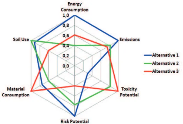
In the Environmental Fingerprint approach, used by BASF Company, the ecological parameters are represented in the same coordinate system, providing comparative
values of eco-efficiency and dismissing absolute values due their lack of representation in the analysis (Saling et al., 2002).
For illustration, the Fingerprint is plotted in the “radar” graphic, as shown in Fig. 1, and such as presented in the
literature (Bidoki et al., 2006; Garcia-Serna et al., 2007).
As seen, it is divided into six indicators for: Energy
Consumption, Emissions (to air, water and wastes),
Toxicity Potential, Risk, Material Consumption and Soil Use, available in dimensionless form.
Figure 1 shows that the indicators are available
together, but it can be difficult to evaluate qualitatively the best alternative (1, 2, or 3) only by the geometric figure
formed, especially when they are apparently similar. Thus, for the decision-making task for assessing
eco-efficiency, BASF also uses the so-called “Portfolio”, which
aggregates the information reported from Fingerprint and
weighting factors specified according to a relevant criteria (i.e., scientific or social considerations).
METHODOLOGY
In the follow sections, we will describe the methodology
for constructing the eco-efficiency index to be applied to
evaluate the performance of a petrochemical plant.
General idea
As previously mentioned, eco-indicators can be grouped and standardized in dimensionless form. To this end, each environmental impact category is normalized
such that the worst case in each category is specified
with the value one and the others receive a relative value
between zero and one (all the values in the same category
are divided by the highest value of this category – worst
case). So that it is possible to build radar graph that
plays the role of an index and serves as a comparative tool. Thus, the performances of an industrial plant at a particular time can be compared against each other by the area of the polygon generated by the radar graph. In the polygon formed, each axis represents an eco-indicator from the same origin.
The dimensionless form (normalized) eliminates the effects of a measurement scale and allows the joint use
of eco-indicators in the form of a single index. So, it is assumed that all the eco-indicators have the same weight because they are an integral part of the same process and
reflect the operational conditions. Consequently, the worst
normalized environmental indicator is 1 and the best value is closer to 0. Hence, the smaller the area, the better the environmental performance of the petrochemical plant in this period.
Graph radar area
The area of the polygon formed by the radar graph was calculated by the Law of Sines. The area is given by the
sum of the areas of the n triangles in the graph; where n is
the number of eco-indicators.
For this calculation, it is necessary to know the sides
of the triangles (the eco-indicators represent the values of each axis of the radar graph) and the angle formed by the axis and its adjacent axis (so, all angles of the triangle are equal and known by value 2π/n). The curve, which limits the graph joining points of the axis (axis values) represents the third side of each triangle, but has no significance for
the calculation.
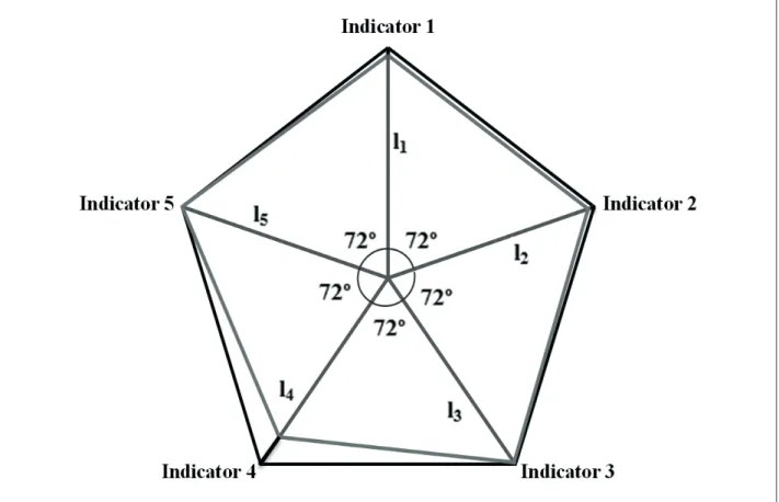
Fig. 2 shows the example of the above description of a
pentagon (n = 5) formed by five triangles, angles of 72° (2 π /5) arranged in the radar graph. The sides of the triangles
are given by l1, l2, l3, l4 and l5, which are the values of the indicators from 1 to 5, respectively.
Law of sines
To calculate the area of the triangles, at least two sides and the angle between them have to be known, to use the
Law of Sines. Fig. 3 displays a triangle ABC of the sides lA, lB and lC and the height denoted as h. θ is the angle formed by the sides lA and lB.
The area of the triangle ABC (SABC) can be calculated
by Equation (1):
(1)
Equation (1) represents the Law of Sines, and will be
used in the proposed methodology. The eco-indicators for the radar graphic are given by the known sides and the central angle.
Calculation of the radar graph area
Applying Equation (1) on the triangle formed by the sides
l1 and l2 in Figure 2, for example, leads to Equation (2).
(2)
In Equation (2) S12 represents the area of the triangle formed by sides 1 and 2. Repeating the procedure for triangles, S23, S34, S45, S51 and adding to S12, it is possible
to obtain the area of the pentagon (ST) formed, as shown
in Equation (3).
(3)
Thus the Eco-efficiency index for the eco-indicators is built.
For n eco-indicators, the expression of eco-efficiency
can be applied generally by Equation (4).
(4)
For a qualitative comparison, it is necessary to evaluate
the radar graph (indexes) of different periods, for example.
According to this, it may be possible to judge whether
there was any increase or decrease of the eco-efficiency over the periods. Thus, the graph with the largest area (S*
T) is the worst environmental scenario.
The Eco-efficiency Comparison Index - ECI - is written according to Equation (5).
(5)
The ECI tool can be extended to any number of eco-indicators and variations, and represents the contribution
of this paper to the eco-indicators field.
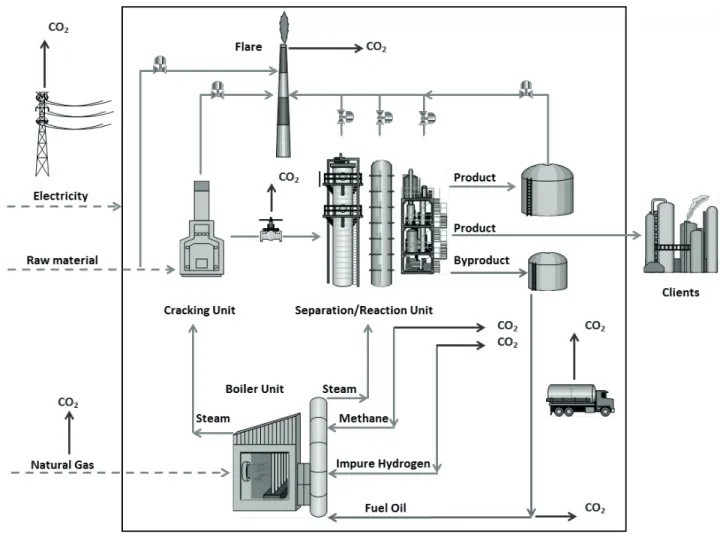
PETROCHEMICAL FACILITY
In this paper the process will be described in a succinct manner. The process analyzed here is represented in Figure 4.
sin
2
A B ABCl
l
S
=
⋅
⋅
θ
1 2 12
2
sin
2
5
l l
S
=
⋅
⋅
⋅
π
12 23 34 45 51
T
S
=
S
+
S
+
S
+
S
+
S
1 1 1 1
1
2
sin
2
nT n i i
i
S
l l
l l
n
π
− + =⋅
= ⋅
⋅
⋅ +
⋅
∑
*1 T 100%
Figure 2. Representation of the polygon in a radar graph, for five categories of indicators.
Figure 3. Representation of any triangle ABC. The raw material (derived from petroleum) is sent
to storage and then processed in a cracker unit, where the hydrocarbon chain reaction occurs, resulting in the desired products. Then, the resulting current is cooled and sent to a separation unit, where the separation of the desired petrochemical products by compression, reaction and distillation processes occurs. These products can be sent directly to the client or stored to be distributed later. Production is recorded daily and split up in accounting by
ducts - totalized by meters (mostly mass type ones) - and by trucks (loaded in storage units) - totalized by weighing. Liquid (fuel oil) and gas fuels (natural gas, methane and impure hydrogen) are sent to the steam boiler along with the electric energy and other inputs (nitrogen, chemistry products and others) are used for the entire unit.
As seen in Fig. 4 the inputs are: raw materials and
supplies of external energy (electricity and natural gas), the processing units (cracking and separation/reaction), and energy generation unit (boiler), which also receives supplies of internal energy (methane, impure hydrogen and residual fuel oil). The outputs are: products and
byproducts, transportation trucks and several process
valves and relief to flare (torch). It is possible to observe,
also, the several sources of energy consumption and CO2 emissions. The water, wastewater and solid waste
are not presented here; details can be found in Pereira
(2013). However, they were considered for monitoring.
With all these variables it was possible to develop the industrial eco-indicators.
Enviromental impact
In this section a complementary study involving the process environmental impacts is explained. LCA attempts to quantify the full range of environmental impacts associated with a product by considering inputs of resources and outputs of wastes and pollution. Typically, such analysis is made at each stage of the product’s life, e.g. acquiring raw materials, production process, transport
In the petrochemical facility analyzed in this paper the ECI is related to the following possible consequences:
(i) global warming (GW), (ii) soil acidification (SA), (iii) photochemical ozone creation (OC) and (iv) human toxicity (HT) (Altamirano, 2013).
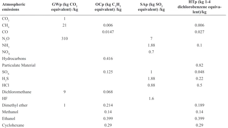
To this end, the following equations were considered: environment impacts
where m1 refers to the mass (in kg per kg of oil) of an ith substance and the subscript p denotes potential impact. A detailed discussion of such indexes can be checked
in Altamirano (2013). Table 1 lists the values of each potential, ω1, related to different substances i (CML, 2001).
As seen, Photochemical ozone creation (OC) for
emission of substances to air is calculated using the
reference unit, kg ethene (C2H4) equivalent. It is the result of reactions that take place between nitrogen oxides
(NOx) and volatile organic compounds (VOC) exposed to
UV radiation (Altamirano, 2013).
Notice that
θ =
im CO
i/
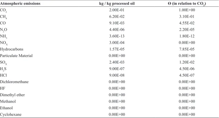
2 is the ratio between each substance in relation to CO2, as shown in Table 2.In order to calculate the GW, SA, OC and HT provoked by the petrochemical facility, we have considered the data
of a typical Brazilian petrochemical facility (Altamirano, 2013), summarized in Table 2.
Table 2 lists the global emission of a typical Brazilian petrochemical facility. Although such values might be
different for distinct plants, those data were used as
reference for a comparative study involving the indexes
represented by Equations (6)-(9) for the present industrial
plant. Wastewater and waste generation are not listed
because they do not affect the indexes GW, SA, OC and HT Figure 4. Overview of a petrochemical industry, the energy and CO2 emission sources (based on Pereira, 2013).
i
GW
GWp
ii
m
=
∑
⋅
(kg CO2 equivalent)i
SA
SAp
ii
m
=
∑
⋅
(kg SO2 equivalent)i
OC
OCp
ii
m
=
∑
⋅
(kg C2H2 equivalent)i
HT
HTp
ii
m
=
∑
⋅
(kg 1-4 dichlorobenzene equivalent) (6)
(7)
(8)
(CML, 2001) sufficiently.
Tables 1 and 2 allow calculating the indexes described by equations 6-9. As observed in Table 2, carbon dioxide is the most representative component in the atmospheric emission. Thus, we have considered CO2 as the key component to compute the quantity of the other substances. According to our results, discussed in the next topic, the CO2 emission can vary with respect to the analyzed period. Thus, to quantify the amount of each component, the CO2
(t/t) emission of each period is multiplied by the standard
CO2 emission listed in Table 2. In this way, the proportion of the other substances in relation to CO2 is kept constant, being estimated indirectly.
RESULTS
For the present analysis, data were collected from a petrochemical plant for seven consecutive months from February to August, 2013. The data acquisition structure
was implemented at the plant site based on Pereira (2013).
Measured data were sent from the Digital Control System
(DCS) to an EXCEL® spreadsheet with the help of an EXCEL® macro with samples of 1 minute. The industrial
data were previously filtered (miscommunications, negative values and corrupted data) and the daily values of
each eco-indicator were then developed by calculating the
amount (generation or consumption) of the environmental
parameters, based on mass and energy balances, and divided by the amount of produced products. Table 3
summarizes the analyzed periods.
The results section is divided in two parts: process
monitoring and eco-efficiency analysis.
Process monitoring results
The month of June has been selected to show how eco-indicators are used for the daily monitoring process.
In the next eco-indicators figures the last plotted result is the accumulative monthly value (Ac.) and it represents the
total of generation or consumption divided by the total of the corresponding production.
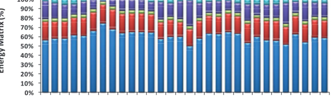
Figs. 5 and 6 illustrate the eco-indicator of Energy Consumption and the Energy Matrix distribution in June 2013, respectively. The target represented in the
figures denotes the operational objectives for a respective production period. Such value is usually defined by the
manager team of the facility. The energy matrix is composed
by: methane, impure hydrogen (mixture of hydrogen and methane), natural gas, electricity and residual fuel oil.
As seen in Fig 5, the energy consumption eco-indicator, on June 2nd, reached the target value of 22.5 GJ/t. It is also possible to observe that the target value was reached on June 13th, 15th, 16th, 17th, 21sh, 26st, 27th, 29th and 30th.
Fig. 6 pictures the energy matrix of the month of June. As observed, the energy matrix is well distributed, including the fuel oil consumption produced at the site plant. However, it is observed in Fig. 7 that the CO2
emission eco-indicator was very high (over the target Table 1. Impact coefficients, ω, (CML, 2001).
Atmospheric
emissions GWp (kg CO2
equivalent) /kg OCp (kg C2
H
2
equivalent) /kg SAp (kg SO2
equivalent) /kg
HTp (kg 1-4 dichlorobenzene equiva
-lent)/kg
CO2 1
CH4 21 0.006 0.006
CO 0.0147 0.027
N2O 310 7
NH3 1.88 0.1
NOX 0.7
Hydrocarbons 0.416
Particulate Material 0.82
SOX 0.125 1 0.048
H2S 1.88 0.22
HCl 0.88 0.5
Dichloromethane 9 0.068
HF 1.6
Dimethyl ether 1 0.214 0.189
Methanol 0.14 0.14
Ethanol 0.399 0.399
value of 0.99 t/t, defined by the manager team of the facility). It can be explained by the failure in the specification of the products, requiring delivery of part of the production to flare. Such result can be confirmed
in Fig.8, which highlights the high percentage of CO2
emissions to flare on June 21st and 26th. As seen, when
the online analysis is over the set point values (safe and specification conditions) the relief valves are
opened. An error in the automation control system was considered after this month. These are two examples of eco-indicators used every day in industry for process monitoring and decision making tasks highlighted in Figs. 5 and 7.
Figs. 7 and 8 illustrate the eco-indicator of CO2 Emission and the CO2 Emissions Matrix distribution in June, 2013, respectively. The CO2 Emissions matrix is composed of the same elements of the energy matrix, plus
the relief to flare emission. A modeling study for all relief valves to flare in this plant has been developed. Thus, given a valve opening, it was possible to estimate the mass flow
through the valve and its corresponding amount in CO2 to atmosphere.
To complete the process monitoring study Figs.9-11
show the Water Consumption, Wastewater Generation and Waste Generation eco-indicators developed, respectively.
Operational conditions reflect on all eco-indicators. On
June 15th and 16th the eco-indicators presented high values due to the temporary reduction in production for inventory adjustment, as shown in Figs. 5, 7, 9-11.
Fig. 11 evidences that the waste is not removed daily. It is performed as operational logistics in function of the waste
accumulation and traffic of trucks in the neighborhood of
the plant site. Further details about these eco-indicators for seven months of monitoring can be found in Pereira
(2013).
Based on the above results, an eco-efficiency comparison index (ECI) has been developed for process
monitoring and decision-making tasks in the petrochemical plant.
Eco-efficiency results
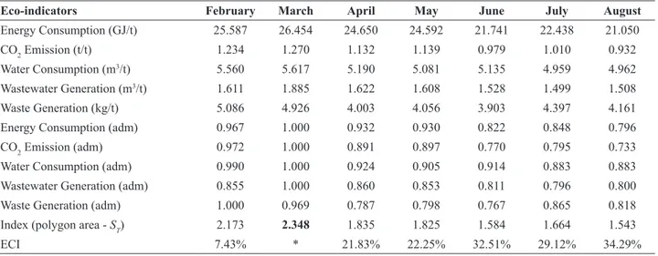
This section presents all monthly accumulated results for each eco-indicator and also the normalized ones in
order to evaluate the eco-efficiency among different
periods. Table 4 summarizes all results for each month.
Table 2. Emissions of a typical Brazilian petrochemical facility (Altamirano, 2013).
Atmospheric emissions kg / kg processed oil ϴ (in relation to CO2)
CO2 2.00E-01 1.00E+00
CH4 6.20E-02 3.10E-01
CO 9.10E-03 4.55E-02
N2O 4.40E-06 2.20E-05
NH3 3.60E-13 1.80E-12
NOX 3.00E-04 0.00E+00
Hydrocarbons 1.57E-05 7.85E-05
Particulate Material 0.00E+00 0.00E+00
SOX 2.40E-03 1.20E-02
H2S 9.00E-07 4.50E-06
HCl 9.00E-08 4.50E-07
Dichloromethane 0.00E+00 0.00E+00
HF 0.00E+00 0.00E+00
Dimethyl ether 0.00E+00 0.00E+00
Methanol 0.00E+00 0.00E+00
Ethanol 0.00E+00 0.00E+00
Cyclohexane 0.00E+00 0.00E+00
Table 3. Summary of the evaluation periods.
Periods Description Months
I Period of observation and setting targets based on historical data. It corresponds to monitoring
before the implementation of the methodology. February and March
II Initial phase of implementing of the method. Started focusing on eco-efficient measures to
improve sustainable development. April, May and June
15 16 17 18 19 20 21 22 23 24 25
01 02 03 04 05 06 07 08 09 10 11 12 13 14 15 16 17 18 19 20 21 22 23 24 25 26 27 28 29 30 Ac.
En
e
rg
y
C
on
su
m
p
ti
on
(G
J/
t)
Target 22.5 GJ/t Day
Figure 5. Eco-indicator of Energy Consumption (June).
0% 10% 20% 30% 40% 50% 60% 70% 80% 90% 100%
01 02 03 04 05 06 07 08 09 10 11 12 13 14 15 16 17 18 19 20 21 22 23 24 25 26 27 28 29 30
En
er
gy
M
atr
ix
(%
)
Methane H2 Eletricity Natural Gas Fuel Oil
Figure 6. Energy Matrix (June).
0.5 0.7 0.9 1.1 1.3 1.5
01 02 03 04 05 06 07 08 09 10 11 12 13 14 15 16 17 18 19 20 21 22 23 24 25 26 27 28 29 30 Ac.
CO
2
E
m
is
sio
n
(
t/
t)
Target 0.99 t/t Day
0% 10% 20% 30% 40% 50% 60% 70% 80% 90% 100%
01 02 03 04 05 06 07 08 09 10 11 12 13 14 15 16 17 18 19 20 21 22 23 24 25 26 27 28 29 30 CO2
M
at
rix
(%)
Methane H2 Eletricity Natural Gas Fuel Oil Flare
Figure 8. CO2 Matrix (June).
3.0 3.5 4.0 4.5 5.0 5.5 6.0 6.5 7.0 7.5
01 02 03 04 05 06 07 08 09 10 11 12 13 14 15 16 17 18 19 20 21 22 23 24 25 26 27 28 29 30 Ac.
W
a
te
r C
o
n
su
m
p
ti
o
n
(
m
³/
t)
Target 5.2 m³/t Day
Figure 9. Eco-indicator of Water Consumption (June).
0.5 0.7 0.9 1.1 1.3 1.5 1.7 1.9 2.1 2.3 2.5
01 02 03 04 05 06 07 08 09 10 11 12 13 14 15 16 17 18 19 20 21 22 23 24 25 26 27 28 29 30 Ac.
W
a
st
ew
a
ter
G
en
er
a
ti
o
n
(m³
/t
)
Target 1.58 m³/t Day
By observing Table 4 it is clear that the two fi rst months
after the production startup were far from the optimal condition. It is possible to note that the ECI increased after March, achieving the highest value in August. However, as observed, in July the eco-indicators of Energy Consumption and CO2 emission increased their values. It was the consequence of the combined factors:
y Sudden unavailability of raw material from external supplier and low storage levels on 17th July;
y Obstruction of one of main heat exchangers and plant intervention maintenance on 18th July;
To maintain the plant operating it was necessary to send to relief valves a considerable amount of processed material and adjust the production to another safe stationary state condition.
These problems are illustrated by the eco-indicator of
CO2 emission in Fig. 12.
Table 4 also reveals that March corresponds to worst case scenario with 2.348 Index value. The comparison between March and August based on the ECI method
shows that the eco-effi ciency increased 34.29%. Other
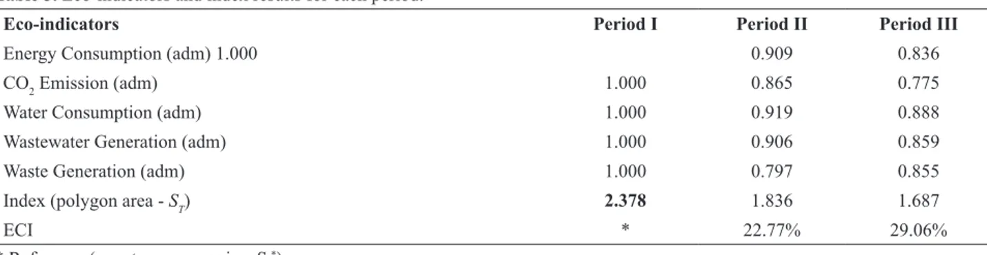
comparison results can also be found in Table 4. To better present the ECI method, Fig. 13 shows the accumulative results for the eco-indicators for the periods I, II and III, respectively, as discussed in Table 3.
Fig. 13 shows the increase of the eco-effi ciency period after
period by the radar graph area decreases. As expected, Period I
(February and March) showed the highest values (1.0).
Table 5 evidences the increase of ECI results from
Period II (April, May, June) to Period III (July and August). As observed, period I corresponds to the worst
case scenario with 2.378 Index value. The comparison between Period I and Period III results based on the ECI
0 2 4 6 8 10 12 14 16 18 20
01 02 03 04 05 06 07 08 09 10 11 12 13 14 15 16 17 18 19 20 21 22 23 24 25 26 27 28 29 30 Ac.
W
a
st
e G
en
er
a
ti
o
n
(k
g
/t
)
Target 4.5 kg/t Day
Figure 11. Eco-indicator of Waste Generation (June). Table 4. Eco-indicators and index results for each month.
Eco-indicators February March April May June July August
Energy Consumption (GJ/t) 25.587 26.454 24.650 24.592 21.741 22.438 21.050
CO2 Emission (t/t) 1.234 1.270 1.132 1.139 0.979 1.010 0.932
Water Consumption (m3/t) 5.560 5.617 5.190 5.081 5.135 4.959 4.962
Wastewater Generation (m3/t) 1.611 1.885 1.622 1.608 1.528 1.499 1.508
Waste Generation (kg/t) 5.086 4.926 4.003 4.056 3.903 4.397 4.161
Energy Consumption (adm) 0.967 1.000 0.932 0.930 0.822 0.848 0.796
CO2 Emission (adm) 0.972 1.000 0.891 0.897 0.770 0.795 0.733
Water Consumption (adm) 0.990 1.000 0.924 0.905 0.914 0.883 0.883
Wastewater Generation (adm) 0.855 1.000 0.860 0.853 0.811 0.796 0.800
Waste Generation (adm) 1.000 0.969 0.787 0.798 0.767 0.865 0.818
Index (polygon area - ST) 2.173 2.348 1.835 1.825 1.584 1.664 1.543
ECI 7.43% * 21.83% 22.25% 32.51% 29.12% 34.29%
0.5 1.0 1.5 2.0 2.5 3.0 3.5
01 02 03 04 05 06 07 08 09 10 11 12 13 14 15 16 17 18 19 20 21 22 23 24 25 26 27 28 29 30 31 Ac.
CO
2
E
m
is
sio
n
(
t/
t)
Target 0.99 t/t Day
Figure 12. Eco-indicator of CO2 emissions (July).
Table 5. Eco-indicators and index results for each period.
Eco-indicators Period I Period II Period III
Energy Consumption (adm) 1.000 0.909 0.836
CO2 Emission (adm) 1.000 0.865 0.775
Water Consumption (adm) 1.000 0.919 0.888
Wastewater Generation (adm) 1.000 0.906 0.859
Waste Generation (adm) 1.000 0.797 0.855
Index (polygon area - ST) 2.378 1.836 1.687
ECI * 22.77% 29.06%
* Reference (worst case scenario - ST*).
method indicates that the eco-effi ciency increased 29.06%.
The results of the Period III, when the ECI presented the best value, can be explained by the fact that some actions were taken together with the operational team:
y Meetings of multidisciplinary teams for better decision
making tasks;
y Engagement of the people, especially the operation team; y Local improvements;
y Adjust the control loops on product specifi cation issue
for relief to fl are;
y Adjust the online chromatograph meter for accuracy
measures;
y Adjust the control loops on security issue for relief to
fl are;
y Detection of leaks in the cooling water and wastewater
systems;
y Detection of leaks in steam lines.
With the eco-indicators, it was possible to observe the production process widely and locally, seeking
eco-effi cient improvements.
Enviromental impact results
Analysis of the GW, SA, OC and HT indexes can be checked in Figure 14 and Figure 15. As observed, CO2 emission is the major cause of global warming, as expected.
As seen, the environmental impact indicators (OC, SA and HT) also decrease with the reduction of CO2 emission. Such analysis agrees with the data listed in Tables 1 and 2 because the ratio of each substance in relation to CO2 is
considered constant in our analysis. Therefore, the profi les
present the same tendency.
The results of Figures 14 and 15 also clarify that the environmental impact could be decreased, principally after the actions taken in period III. Such results highlight the importance of process monitoring, which was possible after the implementation of the ECI.
In order to evaluate the impact of each substance over GW, OC, SA and HT, a sensitivity analysis was done. The results are presented in Figures 16, 17, 18 and 19.
For sensitivity analysis we considered the complete
Brazilian Journal of Chemical Engineering C. P. Pereira, D. M. Prata, L. S. Santos and L. P. C. Monteiro 82
Figure 14. Environmental impact (OC, AS and HT) profiles (the dark region corresponds to the period III).
Figure 15. Environmental impactGW profile (the dark region corresponds to the period III).
standard CO2 levels presented in Table 2. Such study was conducted for the period I.
The summary of the results illustrated in Figures 16, 17, 18 and 19 evidences that:
y The global warming (GW) may be reduced by
minimization of CH4;
y The ozone creation (OC) may be reduced by
Figure 16. Effect of CH4 reduction over (a) GW, (b) SA, (c) OC, and (d) HT for Period I (0% - 100% of substance emission in relation to Table 2).
(a)
(b)
(c)
Figure 17. Effect of CO reduction over (a) GW, (b) SA, (c) OC and (d) HT for Period I (0% - 100% of substance emission in relation to Table 2).
(a)
(b)
(c)
Figure 18. Effect of NOX reduction over (a) GW, (b) SA, (c) OC and (d) HT for Period I (0% - 100% of substance emission in relation to Table 2).
(a)
(b)
(c)
Figure 19. Effect of SOX reduction over (a) GW, (b) SA, (c) OC and (d) HT for Period I (0% - 100% of substance emission in relation to Table 2).
(a)
(b)
(c)
y The soil acidification (SA) may be reduced by
minimization of NOX and SOX;
y The human toxicity (HT) may be reduced by
minimization of CH4, CO and SOX.
Based on the above results, several recommendations
are made to improve the eco-efficiency of the studied
petrochemical plant:
y Plant use of non-carbon-based energy sources; y Reducing the carbon content from fuels;
y Increase the efficiency of heat and power production; y Reducing the amount of wastes flared (Replacing the
valves with greater probability of leakage);
y CO2 capture technologies, such as cryogenic techniques;
y Replacement of the burners of the boiler to allow for burning liquid fuel - fuel oil, byproduct of the process with no great commercial value, in other words, change in the energy matrix, decreasing the importation of
natural gas (external fuel with high monetary cost);
y Best advantage of recyclable waste, lowering disposal; y Plant process optimization. The ECI may be used as
objective function because it includes several indicators
in a unique function). Furthermore, the environmental
impact indexes may be used as constraints of the optimization problem.
y Implementation of data reconciliation for real time data
acquisition (Prata et al, 2010).
CONCLUSIONS
Usually, environmental eco-efficiency is not clearly
observed when measurements are performed with a
single eco-efficiency indicator or indicators evaluated
individually. Therefore, there is a need to develop methods for evaluating the eco-indicator integration, so as to reveal the state of a system or phenomenon and provide a tool for decision-making tasks.
The purpose of the paper was to analyze the
eco-efficiency of a petrochemical plant, suggest eco-eco-efficiency
indexes for measurement of gas emissions, energy loss,
and water waste and propose a global eco-efficiency index
making use of experimental industrial data. The results indicate that some actions taken with the operational team
of the facility could improve the facility eco-efficiency, e.g.: (i) meetings of multidisciplinary teams for better decision-making tasks; (ii) reducing the amount of wastes flared, (iii) avoid leaks in steam lines, (iv) replacement of
the burners of the boiler etc.
An important contribution of this work is certainly developing the methodology for monitoring and process improvement and standardization of eco-indicators in an industrial unit. The development of the comparison tool,
which covers all different ecological indexes, resulting in what has been called eco-efficiency comparison index -
ECI, allows evaluating the environmental performance in
different periods.
Also, a supplementary study was done, evaluating the impacts of atmospheric emissions on the environment:
(i) global warming (GW), (ii) soil acidification (SA), (iii) photochemical ozone creation (OC) and (iv) human toxicity (HT). It was possible to note that global warming is
the main impact caused by the petrochemical industry, and
the associated gasses (SOx, CO and NOx) are extremely
related to the above indexes.
For future studies we suggest: (i) to develop
real-time optimization tools, involving eco-indicators as the objective function, allowing optimizing of petrochemical
facilities in a more global way, (ii) development of new eco-indicators with different weighting factors, considering
environmental impacts, such as reducing human toxicity.
NOMENCLATURE
h - Height of the triangle.
ECI - Eco - efficiency Comparison Index.
l1 - 1st axis of the radar graph representing the sides of the triangle.
l2 - 2sd axis of the radar graph representing the sides of the triangle.
l3 - 3rd axis of the radar graph representing the sides of the triangle.
l4 - 4th axis of the radar graph representing the sides of the triangle.
l5 - 5th axis of the radar graph representing the sides of the triangle.
lA - Side (A) of the triangle. lB - Side (B) of the triangle. lC - Side (C) of the triangle. n - Number of eco - indicators.
S12 - Area of the triangle that composes the polygon of the
radar graph (axes l1 and l2).
S23 - Area of the triangle that composes the polygon of the
radar graph (axes l2 and l3).
S34 - Area of the triangle that composes the polygon of the
radar graph (axes l3 and l4).
S45 - Area of the triangle that composes the polygon of the
radar graph (axes l4 and l5).
S51 - Area of the triangle that composes the polygon of the
radar graph (axes l5 and l1).
SABC - Area of triangle ABC of sides lA, lB and lC. ST - Total area of the polygon formed in the radar graph. ST* - Total area of the polygon formed in the radar graph - worst case scenario.
θ - Angle formed by the sides lA and lB.
ACKNOWLEDGEMENT
The authors thank CAPES (Coordenação de Aperfeiçoamento de Pessoal de Nível Superior) for
REFERENCES
Altamirano, C.A.A., Análise de ciclo de vida do biodiesel de soja: uma Comparação entre as rotas metílica e etílica, Master Thesis, Escola de Química, Universidae Federal do Rio de Janeiro, Brazil, (2013).
Bidoki, S.M., Wittlinger, R., Alamdar, A.A., Burger, J., Eco-efficiency analysis of textile coating materials. Journal of the Iranian Chemical Society 3, 351-359 (2006).
Borén, T., Methods for aggregation and communication of life cycle inventory data within the framework of eco-efficiency analysis, Master thesis, Department of Energy and Environment, Chalmers University of Technology, Göteborg, Sweden (2008).
Burchart-Korol, D., Czaplicka-Kolarz, K., Smolinskia, A., Eco-efficiency of underground coal gasification (UCG) for electricity production, Fuel, 1, 239-246 (2016).
Cahyandito, M.F., The MIPS Concept (Material Input Per Unit of Service): A Measure for an Ecological Economy, Working Papers in Business, Management and Finance, 200901 (2009).
Callens, I., Tyteca, D., Towards indicators of sustainable development for firms A productive efficiency perspective. Ecological Economics 28, 41-53 (1999).
Charmondusit, K., Development of eco-efficiency indicators for assessment of industrial estate. In: International Conference on Green and Sustainable Innovation. Chiang Rai, Thailand, December (2009).
Charmondusit, K., Keartpakpraek, K., Eco-efficiency evaluation of the petroleum and petrochemical group in the map Ta Phut Industrial Estate, Thailand. Journal of Cleaner Production 19, 241–252 (2011).
CML, An operational guide to the ISO-standards - Part 3: Scientific background (Final report, May 2001). (www. leidenuniv.nl/cml/ssp/projects/lca2/lca2.html#gb)
Cote, R. P., Hall, J., Industrial parks as ecosystems. Journal of Cleaner Production 3, 41-46 (1995).
Garcia-Serna, J., Pérez-Barrigón, L., Cocero, M. J., New trends for design towards sustainability in chemical engineering: Green engineering. Chemical Engineering Journal133, 7-30 (2007).
Ichimura, M., Nam, S., Bonjour, S., Rankine, H., Carisma, B., Qiu, Y., Khrueachotikul, R., Eco-efficiency Indicators: Measuring Resource-use Efficiency and the Impact of Economic Activities on the Environment, Greening of Economic Growth Series, United Nations publication (2009). Jollands, N.G., An ecological econoomics eco-efficiency - theory, interpretation and applications. PhD Thesis, Massey University, Palmerston North (2003).
Ingaramo, A., Heluane, H., Colombo, M., Cesca, M., Water and wastewater eco-efficiency indicators for the sugar cane industry, Journal of Cleaner Production 17, 487–495 (2009). Kharel, G.P., Charmondusit, K., Eco-efficiency evaluation of
iron rod industry in Nepal. Journal of Cleaner Production 16, 1379-1387 (2008).
Liu, X., Zhu, B., Zhou, W., Hu, S., Chen, D., Griffy-Brown, C., CO2 emission in calcium carbide industry: An analysis
of China’s mitigation potential. International Journal of Greenhouse Gas Control 5, 1240-1249 (2011).
Lowe, E., Evans, L. K., Industrial ecology and industrial ecosystems. Journal of Cleaner Production 3, 47-53 (1995). Maxine, D., Marcotte, M., Arcand, Y., Development of
eco-efficiency indicators for the Canadian food and beverage industry. Journal of Cleaner Production 14, 636-648 (2006). Nordheim, E., Barrasso, G., Sustainable development indicators
of the European aluminium industry. Journal of Cleaner Production 15, 275 – 279 (2007).
Park, H-S, Behera, S-K., Methodological aspects of applying eco-efficiency indicators to industrial symbiosis networks, Journal of Cleaner Production, 64, 478-485 (2014).
Pereira, C., P., Development and evaluation of comparison index based on eco-indicators in an industrial plant. Master Dissertation in Chemical Engineering. Federal Fluminense University, Niterói, RJ - Brazil (in portuguese), 2013. Prata, D. M., Schwaab, M., Lima, E. L., Pinto, J. C., Simultaneous
robust data reconciliation and gross error detection through particle swarm optimization for an industrial polypropylene reactor. Chemical Engineering Science 65, 4943-4954 (2010). Rattanapan, C., Suksaroj.T.T., Ounsaneha, W. Development
of Eco-efficiency Indicators for Rubber Glove Product by Material Flow Analysis, Procedia - Social and Behavioral Sciences, 40, 99-106 (2012).
Saling, P., Kicherer, A., Dittrich-Krämer, B., Wittlinger, R., Zombik, W., Schimidt, I., Schrott, W., Schimidt, S., Eco-efficiency analysis by BASF: The method. International Journal of Life Cycle Assessment 7, 203-218 (2002). Siitonen, S., Tuomaala, M., Ahtila, P., Variables affecting energy
efficiency and CO2 emissions in the steel industry. Energy
Policy 38, 2477–2485 (2010).
Silalertruksa, T., Gheewala, S.H., Pongpat, P., Sustainability assessment of sugarcane biorefinery and molasses ethanol production in Thailand using eco-efficiency indicator, Applied Energy, 160, 603 – 609 (2015).
Tahara, K., Sagisaka, M., Ozawa, T., Yamaguchi, K., Inaba, A., Comparison of ‘CO2 efficiency’ between company and industry. Journal of Cleaner Production 13, 1301-1308 (2005).
Tyteca, D., On the measurement of the environmental performance of firms – a literature review and a productive efficiency perspective. Journal of Environmental Management 46, 281-308 (1996).
Van Caneghem, J., Block, C., Cramm, R., Mortier, R., Vandecasteele, C., Improving eco-efficiency in the steel industry: The ArcelorMittal Gent case. Journal of Cleaner Production 18, 807-814 (2010).
Veleva, V., Ellenbecker, M., Indicators of sustainable production: framework and methodology. Journal of Cleaner Production 9, 519-549 (2001).
Vukadinovic, B., Popovic, I., Dunjic, B., Jovovic, A., Vlajic, M., Stankovic, D., Bajic, Z., Kijevcanin. N., Correlation between eco-efficiency measures and resource and impact decoupling for thermal power plants in Serbia, Journal of Cleaner Production, Journal of Cleaner Production, 138, 264-274 (2016).
Welford, R., Environmental strategy and sustainable development. The corporate challenge for the 21st century. London: Routledge, 224p. (1995).
World Business Council for Sustainable Development (WBCSD), In: Measuring eco-efficiency: A guide to reporting company performance. World Business Council for sustainable development (2000). Available in: http://www.wbcsd.org/ plugins/DocSearch/details.asp. Accessed on: 22/07/2012.
Woon, K.S., Lo, I.M.C., An integrated life cycle costing and human health impact analysis ofmunicipal solid waste management options in Hong Kong usingmodified eco-efficiency indicator, Resources, Conservation and Recycling, 107, 104-114 (2016).
Wu, J. Wu, Z., Hollander, R., The application of Positive Matrix Factorization (PMF) to eco-efficiency analysis, Journal of Environmental Management, 98, 11-14 (2012).
Zhang, B., Wang, Z., Yin, J., Su, L., CO2 emission reduction within Chinese iron & steel industry: practices, determinants and performance. Journal of Cleaner Production, 33, 167-178 (2012).