A New Branching Rule to Solve the Capacitated Lot Sizing and Scheduling
Problem with Sequence Dependent Setups
W.A. DE OLIVEIRA1* and M.O. SANTOS2
Received on December 26, 2016 / Accepted on July 31, 2017
ABSTRACT.In this paper, we deal with the Capacitated Lot Sizing and Scheduling Problem with sequence dependent setup times and costs – CLSD model. More specifically, we propose a simple reformulation for the CLSD model that enables us to define a new branching rule to be used in Branch-and-Bound (or Branch-and-Cut) algorithms to solve this NP-hard problem. Our branching rule can be easily implemented in commercial solvers. Computational tests performed in 240 test instances from the literature show that our approach can significantly reduce the running time to solve this problem using a Branch-and-Cut algorithm of a commercial MIP solver. Therefore, our approach can also improve the performance of other approaches that need to solve partial sub problems of the CLSD model in each iteration, such as Lagrangian approaches and heuristics based on the mathematical formulation of the problem.
Keywords:Lot Sizing, scheduling, Mixed Integer Linear Programming, Branch-and-Bound algorithm.
1 INTRODUCTION
In most production environments, companies need to decide on the size of production lots in order to obtain efficient inventory management and reduce costs. High inventory levels cause high holding costs and low inventory levels may cause undesirable delays in meeting customer demands.
The lot sizing problem (LP) consists of determining the optimal size of production lots with the aim to minimize costs and meet customer demands. The LP has received special attention from researchers due to its importance for the global economy ([10]).
On the other hand, the scheduling problem consists of determining the sequence of production lots in order to minimize the time and cost generated by product changeovers on production lines. When the cost and time generated by product changeovers depends on previously produced items
*Corresponding author: Willy Alves de Oliveira – E-mail: [email protected]
1Instituto de Matem´atica – INMA, Universidade Federal de Mato Grosso do Sul – UFMS, 79070-900 Campo Grande, MS, Brasil.
and the item to be produced, it can be said that there is a sequence-dependent setup time and/or cost structure.
According to [1], when there is a sequence-dependent setup time/cost structure, the decisions about the size of production lots and the sequence of production need to be taken simultane-ously, because the solution obtained by an hierarchical approach may be infeasible or suboptimal. Therefore, the simultaneous lot sizing and scheduling problem (LSP) consists of simultaneously deciding the sizes and production sequences.
In the literature, there are various mathematical models to deal with LSP. We highlight the ca-pacitated lot sizing and scheduling with sequence dependent setups – CLSD model ([13]), the general lot sizing and scheduling problem – GLSP model ([9], [16]) and the reformulation of GLSP model proposed in [5] – CC model. Recent reviews of the models to deal with LSP are presented in [12, 1, 6].
In [12], the authors compare various mathematical models for LSP and by using theoretical and computational results, it could be concluded that the CLSD model is a promising formulation to deal with LSP. The CLSD model has an interesting performance in exact solution approaches such as Brand-and-Bound algorithms from commercial MIP solvers.
In this paper, we introduce a very simple reformulation for the CLSD model (the CLSDwmodel)
that allows us to introduce a new branching rule able to significantly improve the computational performance of this model in Branch-and-Bound (Branch-and-Cut) algorithms. Therefore, our approach can be used to improve the performance of commercial solvers and approaches to deal with LSP that need to solve partial sub problems, such as Lagrangian approaches and MIP based heuristics.
We use a set of 240 test instances from the literature to compare the performance of the tradi-tional CLSD with our approach in a commercial powerful solver Cplex 12.60. Computatradi-tional results show that our approach can significantly improve the performance of the solver Cplex, reducing running time and proving optimality for more test instances. This paper is organized as follows: Section 2 presents a literature review for LSP; Section 3 presents the mathemati-cal formulation CLSDwand the branching rule and Section 4 presents the computational results
comparing the performance of the traditional CLSD model with our approach in the Branch-and-Cut algorithm from Cplex 12.60. Finally, the conclusions and future proposals are presented in Section 5. Details of the computational implementation are given in the appendix.
2 LITERATURE REVIEW
The original GLSP model was reformulated in [20] using a network flow problem structure and in [5] suppressed the setup state variables in the model. Computational tests performed in [12] showed that both reformulations can provide better dual bounds by solving linear relaxation than the dual bounds obtained by solving the linear relaxation of the GLSP model.
In [13], the CLSD model was introduced using another strategy, consisting of introducing con-straints and variables from the travelling salesman problem to map the start time and end time of production of each item in each period, to model the sequencing decisions. The CLSD model considers, originally, a single-stage system where several items have to be produced on a single machine in a finite planning horizon supposing a known dynamic deterministic demand which must be completely satisfied without backlogging.
Mixed integer programming models based on the CLSD model have been proposed to deal with problems from various real world production environments, such as [15], which addressed a yogurt industry and [21], which studied a semiconductor assembly and test manufacturing.
In other papers, extensions of the GLSP model were compared with the extension of the CLSD model to deal with different real problems. For example, [2] addressed the LSP on parallel pro-duction lines that need to be equipped with tools for processing. Models inspired by GLSP and CLSD were developed to synchronize these tools on the production lines. Computational tests showed that the CLSD model has a much better performance than the GLSP model considering the runtime and the ability to find feasible solutions.
Computational tests in [12] showed that the CLSD model performs better than all the models that use micro period structures. In particular, the CLSD model presented a lower average devi-ation from the best known solution (GAP) and running time than other models.
The LSP is aNP-completeproblem ([9, 16, 17]) where instances based on real world problems can be difficult to solve by exact algorithms at an acceptable computational time. Therefore, various heuristic approaches have been developed to deal with the LSP. For example, [13] pro-posed a backward oriented heuristic to solve the LSP model without setup times, while [17] proposed a threshold accepting methaheuristic to deal with LSP considering sequence dependent setup times.
Heuristics based on the mathematical formulation of the problem (MIP based heuristics) have been frequently used to solve the LSP, in particular, therelax-and-fix – RFandfix-and-optimise – FO. FO heuristics have obtained good solutions for various types of lot sizing and scheduling problems and various heuristics approaches combining RF and FO heuristics have been proposed in the literature, such as [3, 7, 8, 22, 19].
The FO is an improvement heuristic that starts in any feasible solution and in each iteration a subset of binary variables are re-optimized while the other binary variables have their values fixed on the value of the incumbent solution. For lot sizing and scheduling problems, the most used variable partitions are by periods, products and production lines. FO heuristics can also be used with an exact method (matheuristics). For example, [11] combined FO with column generation and [4] integrated FO with theVariable Neighbourhood Search – VNSmethaheuristic.
Therefore, as MIP based heuristics solve, in each iteration, a small mixed integer linear pro-gramming model, these heuristics can be improved if a good model and a good exact solution algorithm are used to solve the sub problems in each iteration. Therefore, the reformulation and the branch rule proposed in this paper can improve the computational performance of some MIP based heuristics to deal with LSP.
3 MODEL FORMULATION AND SOLUTION APPROACH
The traditional CLSD model with setup times can be found in [12] and the following parameters and variables are used to define it:
Parameters:
• T: number of periods (indexed byt);
• J: number of items (indexed byiand j);
• dj t: demand of item jin periodt;
• Ct: available capacity time in periodt;
• aj: consumed capacity time for production of a unit of item j;
• hj: inventory cost of item j;
• sci j: setup cost for exchange between itemsiand j;
• sti j: setup time for exchange between itemsiand j;
Variables:
• Ij t: inventory of item jat the end of periodt;
• xj t: produced quantity of item jin periodt;
• Vj t: production order of itemj in periodt;
• yj s: 1, if the item jis the first item produced in periodtand 0, otherwise;
The CLSD model is given by (3.1) to (3.10).
Min
J
j=1
T
t=1
hjIj t+ J
i=1
J
j=1
T
t=1
sci j tzi j t (3.1)
subject to Ij,t−1+xj t =dj t+Ij t, ∀t, (3.2) J
j=1 ajxj t+
J
i=1
J
j=1
sti jzi j t ≤Ct, ∀t, (3.3)
xj t ≤
Ct
aj
yj t+ J
i=1 zi j t
, ∀j,t, (3.4)
J
j=1
yj t =1, ∀t, (3.5)
yj t + J
i=1 zi j t =
J
i=1
zj it +yj,t+1, ∀j, (3.6)
Vj t ≥Vit+1−J(1−zi j t), ∀i,j,t, (3.7)
Ij t,Vj t,xj t ≥0, ∀j,t, (3.8)
yj t ∈ {0,1}, ∀j,t, (3.9)
zi j t ∈ {0,1}, ∀i,j,t. (3.10)
The objective function (3.1) reflects the sum of holding costs and product changeover costs, while (3.2) are the inventory balance constraints and (3.3) are the capacity constraints. Con-straints (3.4) ensure that item j can only be produced if the production line is set up for it. Constraints (3.5) ensure that only one item is the first produced item in each period, while constraints (3.6) trace the machine configurations. Constraints (3.7) are MTZ (Miller-Tucker-Zemlin) constraints to eliminate sub tours and, finally, constraints (3.8) -(3.10) define the domain of decision variables.
To introduce our branching rule, we firstly define a reformulation of the CLSD model called the CLSDw model. Consider new binary variableswj t, wherewj t = 1, if item j is produced in
periodtandwj t =0, otherwise. Clearly, we have that
wj t =yj t + J
i=1
zi j t, ∀j,t. (3.11)
Note that, by (3.11) ifwj t = 1, then the item j must be scheduled in periodt, implying in a
setup cost. Therefore, ifxj t =0 then in the optimal solution we have thatwj t =0.
The CLSDwmodel can be obtained introducing constraints (3.11) and (3.13) in the CLSD model and replacing constraints (3.4) by constraints (3.12), where:
xj t ≤
Ct
aj
wj t, ∀j,t, (3.12)
3.1 Branching rule
Note that by (3.11), ifwj t = 0, thenyj t =0,zi j t =0 andzj it =0,∀i. Therefore, if we can
identify that item jis not produced in one period, we can fix directly the value of 2J+1 binary variables on zero.
This fact motivated us to introduce the binary variableswj t in the CLSD model, obtaining the
CLSDw model, and performing a branch-and-bound algorithm with a priority of branching for these variables. Note that this reformulation increases the number of binary variables inJ ∗T, however it enables us to perform a more efficient branching scheme in a branch-and-bound or branch-and-cut algorithm.
In each search tree node, given an optimal solution of linear relaxation, our branching rule is: if there are variableswj t with no integer values, we firstly perform the branching in these variables
before variablesyj t andzi j t.
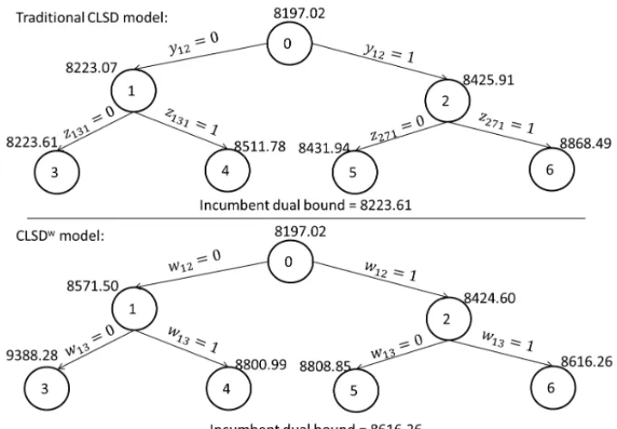
Figure 1 presents an example comparing a traditional branch-and-bound algorithm in the CLSD model and a branch-and-bound algorithm using the CLSDwmodel with our branching rule. The
instance considered in Figure 1 has 15 products and 5 periods and we notice that with just six nodes explored, the incumbent dual bound found with our branching rule is significantly bet-ter than the best dual bound found in a traditional branching scheme. In this test instance, the traditional branch-and-bound algorithm consumed around 56 seconds to solve the CLSD model to optimality, while the branch-and-bound algorithm with the branching rule introduced in this paper consumed only around 6 seconds to solve the CLSDwmodel.
We empirically observe that with some values of variableswj t fixed in binary numbers, the value
of linear relaxation for variables yj t andzi j t also tends to be binary. Clearly, ifwj t =0, then
yj t =0, zi j t =0 andzj it =0,∀i (see (3.11)). Consider now a simplified case where just two
items can be produced in each period and suppose that in a given node, the values of variables
wit andwj t were fixed in one for somei,j andt. Suppose thatsti j < stj i andsci j < scj i.
Therefore, in the optimal solution of the linear relaxation in this node, we will have yit = 1,
yj t =0,zi j t =1 andzj it =0.
Our branching scheme has another advantage. It can be easily implemented using a commer-cial solver, and therefore, we can benefit from a general powerful branch-and-cut algorithm and various general heuristics to improve the convergence.
In Section 4, we present computational results to compare the performance of the traditional CLSD model with the performance of the CLSDw model using our branching scheme imple-mented in the Cplex 12.60 solver on 240 test instances from the literature.
4 COMPUTATIONAL RESULTS 4.1 Test environment
We implemented the traditional CLSD model, the CLSDw model and our branching rule in C++ language using the library Concert Technology of the Cplex 12.60 solver. We denote by CLSDwB Rthe results of the model CLSDw using our branching rule in the general Branch-and-Cut algorithm of the Cplex solver.
We ran the tests on a computer with two Intel Xeon processors, 2.8 GHz and 128 GB DDR3 RAM memory. The maximum running time was fixed to one hour (3600 seconds). For each instance, we captured the best feasible solution and the best dual bound found. The deviation of the best feasible solution from the lower bound (GAP) was computed asG AP =100∗zf−zd
zf
, where
zf is the best feasible solution andzdis the incumbent dual bound.
4.2 Test instance features and computational results
To test the performance of model CLSDw with our branching rule, we used a set of 240 test instances from the literature, and compared it with the performance of traditional CLSD model. The test instances were presented in [14] and can be obtained inhttp://www.mang.canterbury. ac.nz/people/rjames. The test instances have the following features:
1. J∈ {15,25},T ∈ {5,10,15};
2. hj ∈ {2, . . . ,9};
3. dj t ∈ {40, . . . ,59};
4. sti j ∈ {5, . . . ,10}andsci j =θsti j, whereθis a positive parameter;
5. aj =1;
6. Ct =
jdj t
Another parameterCut V arwas introduced in order to control the amount of capacity variation. The parameterCut V ar represents and controls the maximum total allowed variation fromCut, and therefore the actual capacity can vary ([14]). The value forCut V ar was fixed to 0.5 for all the test instances as in [14].
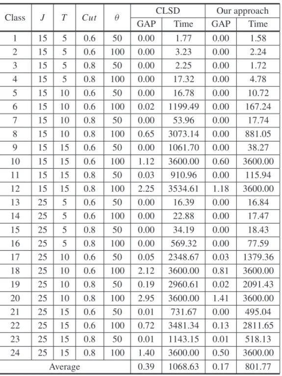
The test instances were grouped into twenty four classes, with 10 test instances each class, ac-cording to the value of parameters J,T,Cut,Cut V arandθ. The values of parameters for each class and the results are given in Table 1 while the results grouped by number of products (J), number of periods (T) and capacity utilization (Cut) are presented in Table 2.
Table 1: Test instances features and computational results.
CLSD Our approach
Class J T Cut θ
GAP Time GAP Time
1 15 5 0.6 50 0.00 1.77 0.00 1.58
2 15 5 0.6 100 0.00 3.23 0.00 2.24
3 15 5 0.8 50 0.00 2.25 0.00 1.72
4 15 5 0.8 100 0.00 17.32 0.00 4.78
5 15 10 0.6 50 0.00 16.78 0.00 10.72
6 15 10 0.6 100 0.02 1199.49 0.00 167.24
7 15 10 0.8 50 0.00 53.96 0.00 17.74
8 15 10 0.8 100 0.65 3073.14 0.00 881.05 9 15 15 0.6 50 0.00 1061.70 0.00 38.27 10 15 15 0.6 100 1.12 3600.00 0.60 3600.00 11 15 15 0.8 50 0.03 910.96 0.00 115.94 12 15 15 0.8 100 2.25 3534.61 1.18 3600.00
13 25 5 0.6 50 0.00 16.39 0.00 16.84
14 25 5 0.6 100 0.00 22.88 0.00 17.47
15 25 5 0.8 50 0.00 34.19 0.00 18.43
16 25 5 0.8 100 0.00 569.32 0.00 77.59
17 25 10 0.6 50 0.05 2348.67 0.03 1379.36 18 25 10 0.6 100 2.12 3600.00 0.81 3600.00 19 25 10 0.8 50 0.19 2960.61 0.02 2091.43 20 25 10 0.8 100 2.95 3600.00 1.41 3600.00 21 25 15 0.6 50 0.01 731.67 0.00 495.04 22 25 15 0.6 100 0.72 3481.34 0.13 2811.65 23 25 15 0.8 50 0.01 1143.15 0.01 518.13 24 25 15 0.8 100 1.40 3600.00 0.50 3600.00
Average 0.39 1068.63 0.17 801.77
Table 2: Results by parameters.
GAP(%) Time (sec) Optimality
CLSD CLSDwB R CLSD CLSDwB R CLSD CLSDwB R
J
15 0.34 0.15 1041.25 703.44 91 100
25 0.62 0.24 1842.35 1518.83 66 76
T
5 0.00 0.00 83.42 17.58 80 80
10 0.75 0.28 2106.58 1468.44 40 54
15 0.69 0.30 2135.40 1847.38 37 42
Cut
0.6 0.34 0.13 1258.64 1011.70 84 91
0.8 0.62 0.26 1624.96 1210.57 73 85
= 0.39 and GAPC L S Dw
B R = 0.17), while the general average time was reduced by around 24% (TimeC L S D =1068.63 and TimeC L S Dw
B R= 801.77).
The average time was reduced by 19 classes, remaining constant in 4 classes and increased in only one class (class 12). The increase is due to an instance from class 12 the random access memory limit (128 GB) was exceeded before reaching the time limit by the traditional CLSD model, and therefore, the running time was slightly reduced. The largest reduction in the average time occurred in classes 6, 11 and 16 where our approach reduces the mean running time by around 86%. In Table 2, it can be observed that our approach could prove optimality in 176 test instances while the traditional approach could prove optimality in 157 test instances.
Table 2 shows that when the number of products or periods increased, then the problem becomes more difficult to solve resulting in longer average deviations and running times, as well as a reduction in the number of instances considering optimality. This fact is not impressive, because the branch-and-cut algorithm grows exponentially when the number of decisions is increased.
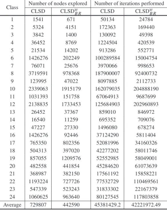
Table 3 presents the number of nodes explored in the search and the number of iterations (in-cluding the cuts applied). We can observe that using our branching rule, the average number of nodes explored was reduced by around 39%, while the average number of iterations was reduced by around 6.9%.
The number of nodes explored in the CLSDwB Rapproach was greater than CLSD approach for classes 13, 17, 19 and 21 and it was smaller for the other classes. Considering only the classes in which all instances were solved to optimality, the number of nodes explored in the CLSDwB R approach was around 76% smaller than the number of nodes explored in the CLSD approach. Considering the classes with residual GAPs, the number of nodes explored in the CLSDwB R approach was around 11% smaller than CLSD approach.
Table 3: Number of nodes and iterations performed.
Number of nodes explored Number of iterations performed Class
CLSD CLSDwB R CLSD CLSDwB R
1 1541 671 50134 24784
2 5324 4151 172363 169440
3 3842 1400 130092 49398
4 36452 8769 1224504 420539
5 21534 14202 913286 552771
6 1426276 202249 100289584 15004754
7 76071 25676 3970066 998653
8 3719591 978368 187900007 92400732
9 123995 47022 8097885 2112733
10 2339063 1915179 162079035 204888190
11 1031393 151758 67064913 9687699
12 2138835 1733453 125684903 202960893
13 26452 37367 859010 846972
14 16540 11259 695352 709076
15 47227 27330 1496080 678274
16 1426276 92446 37124290 5811404
17 765350 802356 52081996 34160326
18 504313 397020 42277202 58011746
19 857055 1209576 52552985 58049001
20 482558 441854 45284620 61073639
21 368987 382150 17561192 15858221
22 1193224 727726 77532729 110469561
23 547339 523243 31833302 22167379
24 1060625 963640 80127545 117803858
Average 729807 442590 45381429.2 42221972.49
4.3 Impact of the proposed branching rule
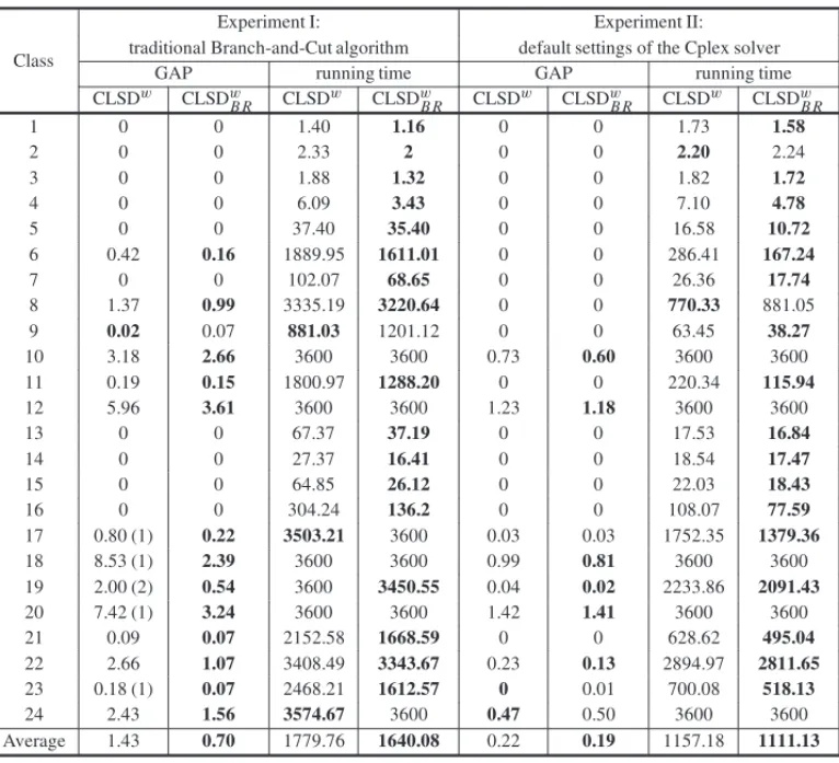
In this section we present some results to try to identify the impact of the branching rule proposed considering the results obtained in Section 4.2. Table 4 presents results with the aim of comparing the performance of the model with the branching rule (CLSDw
Table 4: Studing the impact of the proposed branching rule.
Experiment I: Experiment II:
traditional Branch-and-Cut algorithm default settings of the Cplex solver Class
GAP running time GAP running time
CLSDw CLSDwB R CLSDw CLSDwB R CLSDw CLSDwB R CLSDw CLSDwB R
1 0 0 1.40 1.16 0 0 1.73 1.58
2 0 0 2.33 2 0 0 2.20 2.24
3 0 0 1.88 1.32 0 0 1.82 1.72
4 0 0 6.09 3.43 0 0 7.10 4.78
5 0 0 37.40 35.40 0 0 16.58 10.72
6 0.42 0.16 1889.95 1611.01 0 0 286.41 167.24
7 0 0 102.07 68.65 0 0 26.36 17.74
8 1.37 0.99 3335.19 3220.64 0 0 770.33 881.05
9 0.02 0.07 881.03 1201.12 0 0 63.45 38.27
10 3.18 2.66 3600 3600 0.73 0.60 3600 3600
11 0.19 0.15 1800.97 1288.20 0 0 220.34 115.94
12 5.96 3.61 3600 3600 1.23 1.18 3600 3600
13 0 0 67.37 37.19 0 0 17.53 16.84
14 0 0 27.37 16.41 0 0 18.54 17.47
15 0 0 64.85 26.12 0 0 22.03 18.43
16 0 0 304.24 136.2 0 0 108.07 77.59
17 0.80 (1) 0.22 3503.21 3600 0.03 0.03 1752.35 1379.36
18 8.53 (1) 2.39 3600 3600 0.99 0.81 3600 3600
19 2.00 (2) 0.54 3600 3450.55 0.04 0.02 2233.86 2091.43
20 7.42 (1) 3.24 3600 3600 1.42 1.41 3600 3600
21 0.09 0.07 2152.58 1668.59 0 0 628.62 495.04
22 2.66 1.07 3408.49 3343.67 0.23 0.13 2894.97 2811.65
23 0.18 (1) 0.07 2468.21 1612.57 0 0.01 700.08 518.13
24 2.43 1.56 3574.67 3600 0.47 0.50 3600 3600
Average 1.43 0.70 1779.76 1640.08 0.22 0.19 1157.18 1111.13
The Cplex solver (using default settings) triggers heuristics to identify the nodes that must be explored first, i.e., the Cplex solver can infer branching rules by exploring the structure of the CLSDw model. In this way, with the aim of better understanding the impact of the branching rule, we performed Experiment I turning off all existing heuristics and presolve techniques in the Cplex solver obtaining a traditional Branch-and-Cut algorithm.
We can observe in the results from Experiment I shown in Table 4 that the use of the branching rule causes a reduction in the general average GAP of around 51% (GAPC L S Dw = 1.43 and GAPC L S Dw
B R= 0.70) and a reduction in the average running time of around 7.80% (TIMEC L S Dw = 1779.76 and TIMEC L S DwB R = 1640.08).
seconds, while without the rule, the average running time was around 347 seconds. Therefore, our approach reduces the time needed to solve these instances to optimality by around 8.8%.
We also observe that, without the branching rule, no feasible solutions were found for 6 instances, while using the rule, feasible solutions were found for all test instances. The number of instances that the CLSDw approach could not find a feasible solution is given in parenthesis in the GAP column of Experiment I in Table 4.
In Classes 17 and 24, the running time for CLSDw was less than that for CLSDwB R, because the RAM memory limit was exceeded before the timeout expired for some instances in the CLSDw
model without our branching rule.
Experiment II was performed using default settings of the Cplex solver with the aim of to identify the impact of our branching rule when heuristics are used (in the background) to determine the nodes to be explored. We can observe in Table 4 that the use of our branching rule causes a re-duction of approximately 10% in the average GAP (GAPC L S Dw= 0.22 and GAPC L S Dw
B R = 0.19) and a reduction in the average running time (TIMEC L S Dw= 1157.18 seconds and TIMEC L S Dw
B R = 1111.13 seconds) of around 4%.
It can be observed that, considering only the instances in which the optimal solution was found (from classes 1 to 9, 11, 13 to 16, 21 and 23) in Experiment II, the average running time without the branching rule is 192 seconds and, using the rule, this time is 158 seconds. Therefore, the time needed to solve these instances to optimality was reduced by around 17% when our branching rule was used.
Experiments I and II showed that our branching rule causes a positive impact in the computational performance of the CLSDw model. This impact is more evident when a traditional Branch-and-Cut algorithm is used. However, even using heuristics to determine the nodes that are explored (default settings of the Cplex solver), making our branching rule explicit can significantly accel-erate the computational convergence of the Branch-and-Cut algorithm.
5 CONCLUSIONS AND FUTURE STUDIES
In this paper, we deal with the lot sizing and scheduling problem with sequence dependent setup costs and times. We proposed a simple reformulation for the CLSD model originating the CLSDw model. The CLSDwmodel consists of explicitly specifying the binary variables (w) to indicate if an item is produced in one period or not. This formulation allowed us to define a new branching rule to improve the performance of branch-and-bound algorithms. Our branching rule consists of firstly performing the branching in variableswbefore the other binary variables. We implemented the CLSDw model and our branching rule in the Cplex 12.60 solver, tested
The branching rule proposed in this paper can improve the performance of algorithms that need to partially solve the CLSD model in each iteration, such as the mixed integer programming based heuristics and Lagrangian based heuristics. As future studies, we highlight the investigation of these approaches using the CLSDwmodel with the branching rule proposed in this paper.
ACKNOWLEDGEMENTS
The authors would like to thank the following funding agencies for the financial support: Con-selho Nacional de Desenvolvimento Cient´ıfico e Tecnol´ogico (CNPq), and Fundac¸˜ao de Amparo Pesquisa do Estado de S˜ao Paulo (FAPESP) via CEPID No. 2013/07375-0.
APPENDIX: COMPUTATIONAL IMPLEMENTATION
According to the Cplex User’s Manual, in the search, Cplex makes decisions about which able to branch on at a node and the user can control the order in which Cplex branches on vari-ables by issuing a priority order. Cplex performs branches on varivari-ables with a higher assigned priority number before variables with a lower priority number.
From Concert Technology, the user can set priority for variables using the methodsetPriority. By default, the variables not assigned an explicit priority value by the user are treated as having a priority value of zero. In this way, our branching rule can be implemented setting a higher priority for variableswj t,∀j,t,than the other binary variables. In this paper, we set a priority of
2 for all variableswj t and use the default value (0) for all variablesyj t andzi j t.
We provide the complete code in C++ language including the implementation of the models and the branching rule on the websitehttp://conteudo.icmc.usp.br/pessoas/mari/
Pesquisas.htm.
RESUMO.Neste artigo tratamos do desafiador problema integrado de dimensionamento de
lotes e sequenciamento da produc¸˜ao na existˆencia de tempos e custos de preparac¸˜ao para produc¸˜ao dependentes da sequˆencia. Mais especificamente, nossa atenc¸˜ao ´e fixada no
mo-delo CLSD, proposto em [13]. Prop˜oe-se, neste trabalho, uma reformulac¸˜ao para o momo-delo
CLSD (intitulada CLSDw), bem como, uma nova regra debranchingpara ser utilizada em algoritmos do tipoBranch-and-Boundpara soluc¸˜ao do modelo CLSDw. Por meio de testes
computacionais realizados com base em instˆancias da literatura, foi poss´ıvel observar que a
abordagem de soluc¸˜ao proposta neste artigo ´e bastante promissora, uma vez que proporcionou significante reduc¸˜ao no tempo computacional para soluc¸˜ao problema, elevada reduc¸˜ao no
desvio m´edio (GAP) entre a melhor soluc¸˜ao e o melhor limitante dual conhecidos e uma significante elevac¸˜ao no n´umero de instˆancias resolvidas at´e a otimalidade quando comparado
com a abordagem tradicional.
REFERENCES
[1] B. Almada-Lobo et al. Industrial insights into lot sizing and scheduling modeling.Pesquisa Opera-cional,35(3) (2015), 439–464.
[2] C. Almeder & B. Almada-Lobo. Synchronisation of scarce resources for a parallel machine lotsizing problem.International Journal of Production Research,49(24) (2011), 7315–7335.
[3] S.A. de Araujo, M.N. Arenales & A.R. Clark. Lot sizing and furnace scheduling in small foundries.
Computers & Operations Research,35(3) (2008), 916–932.
[4] H. Chen. Fix-and-optimize and variable neighborhood search approaches for multi-level capacitated lot sizing problems.Omega,56(2015), 25–36.
[5] A.R. Clark & S.J. Clark. Rolling-horizon lot-sizing when set-up times are sequence-dependent. Inter-national Journal of Production Research,38(10) (2000), 2287–2307.
[6] K. Copil et al. Simultaneous lotsizing and scheduling problems: a classification and review of models.
OR Spectrum,39(1) (2017), 1–64.
[7] D. Ferreira, R. Morabito & S. Rangel. Solution approaches for the soft drink integrated production lot sizing and scheduling problem.European Journal of Operational Research,196(2) (2009), 697–706.
[8] D. Ferreira, R. Morabito & S. Rangel. Relax and fix heuristics to solve one-stage one-machine lot-scheduling models for small-scale soft drink plants.Computers & Operations Research,37(4) (2010), 684–691.
[9] B. Fleischmann & H. Meyr. The general lotsizing and scheduling problem. Operations-Research-Spektrum,19(1) (1997), 11–21.
[10] C.H. Glock, E.H. Grosse & J.M. Ries. The lot sizing problem: A tertiary study.International Journal of Production Economics,155(2014), 39–51.
[11] L. Guimaraes, D. Klabjan & B. Almada-Lobo. Pricing, relaxing and fixing under lot sizing and scheduling.European Journal of Operational Research,230(2) (2013), 399–411.
[12] L. Guimar˜aes, D. Klabjan & B. Almada-Lobo. Modeling lotsizing and scheduling problems with sequence dependent setups.European Journal of Operational Research,239(3) (2014), 644–662.
[13] K. Haase. Capacitated lot-sizing with sequence dependent setup costs. Operations-Research-Spektrum,18(1) (1996), 51–59.
[14] R.J.W. James & B. Almada-Lobo. Single and parallel machine capacitated lotsizing and schedul-ing: New iterative MIP-based neighborhood search heuristics.Computers & Operations Research,
38(2011), 1816–1825.
[15] G.M. Kopanos, L. Puigjaner & C.T. Maravelias. Production planning and scheduling of parallel con-tinuous processes with product families.Industrial & engineering chemistry research,50(3) (2010), 1369–1378.
[16] H. Meyr. Simultaneous lotsizing and scheduling by combining local search with dual reoptimization.
European Journal of Operational Research,120(2) (2000), 311–326.
[17] H. Meyr. Simultaneous lotsizing and scheduling on parallel machines.European Journal of Opera-tional Research,139(2) (2002), 277–292.
[19] W. Wei et al. Tactical production and distribution planning with dependency issues on the production process.Omega,67(2017), 99–114.
[20] L.A. Wolsey. MIP modelling of changeovers in production planning and scheduling problems. Euro-pean Journal of Operational Research,99(1) (1997), 154–165.
[21] J. Xiao et al. A hybrid Lagrangian-simulated annealing-based heuristic for the parallel-machine capacitated lot-sizing and scheduling problem with sequence-dependent setup times.Computers & Operations Research,63(2015), 72–82.
[22] S. C¸ a ˘grı & B. Bilgen. Hybrid simulation and MIP based heuristic algorithm for the production and