doi: 10.1590/0101-7438.2015.035.03.0439
INDUSTRIAL INSIGHTS INTO LOT SIZING AND SCHEDULING MODELING*
Bernardo Almada-Lobo
1**, Alistair Clark
2, Lu´ıs Guimar˜aes
1,
Gonc¸alo Figueira
1and Pedro Amorim
1Received October 12, 2015 / Accepted November 30, 2015
ABSTRACT.Lot sizing and scheduling by mixed integer programming has been a hot research topic in the last 20 years. Researchers have been trying to develop stronger formulations, as well as to incorporate real-world requirements from different applications. This paper illustrates some of these requirements and demonstrates how small- and big-bucket models have been adapted and extended. Motivation comes from different industries, especially from process and fast-moving consumer goods industries.
Keywords: lot sizing and scheduling, mixed integer programming, industrial applications, real-world features.
1 INTRODUCTION
Production planning and scheduling seeks to efficiently allocate resources while fulfilling cus-tomer requirements and market demand, often by trading-off conflicting objectives. Lot sizing and scheduling (L&S) is one of the most important and challenging processes within the produc-tion planning of an industrial company, which is done under a hierarchical process with several stages, each containing different aims and planning horizons. According to the Supply Chain Planning (SCP) matrix (e.g. Fleischmann & Meyr, 2003), L&S is of short/medium-term scope and is placed between Master Production Scheduling and Operational Scheduling.
Integrating lot sizing and scheduling is crucial for many companies (Clark et al., 2011). Lot sizing determines the timing and level of production to meet product demand over a finite plan-ning horizon. Sequencing establishes the order in which lots are executed within a time period, accounting for the sequence dependent setup times and costs. The motivation for integrating these two problems may come from:
*Invited paper. **Corresponding author.
1INESC TEC and Faculdade de Engenharia, Universidade do Porto, Porto, Portugal.
– E-mails: [email protected]; [email protected]; [email protected]; [email protected] 2University of the West of England, Department of Engineering Design and Mathematics, Bristol, UK.
a) the optimality point-of-view – creating more cost efficient production plans than those obtained when solving the two problems hierarchically by inducing the solution of the lot sizing problem at the scheduling level;
b) the feasibility point-of-view – in many production environments, due to the extremely tight production capacity, creating implementable production plans is challenging without this integrated approach.
The integration of L&S is required in production environments that usually share the following characteristics (Kallrath, 2002): multi-product equipment, significant sequence-dependent setup times and costs, divergent bill of materials, multi-stage production, typically with a known sta-tionary bottleneck, and combined batch production and continuous operations. This is the case in many process industries. Furthermore, these industries often face strongly seasonal demand, and capacity (usually constant) is insufficient to accommodate these variations. Under the afore-mentioned conditions just-in-time systems can not be implemented and a make-to-stock policy is economically preferable over investments in expanding capacity (Pochet, 2001).
The recent developments in hardware and in the computational efficiency of modern commercial solvers have allowed researchers to propose more complex and realistic mathematical formula-tions for different L&S variants. Furthermore, the trendy and successful research line on mathe-matical programming-based heuristics benefits from stronger formulations. This paper provides an overview of the modeling features and extensions to address different requirements motivated by industrial applications of L&S. Special attention is given to the modeling perspective rather than solution approaches. The paper overviews the main modeling extensions by focusing on setup operations, synchronizing production resources, product features, and planning process characteristics. These extensions are discussed for the two most well-known L&S models: the Capacitated Lot Sizing Problem with sequence-dependent setups (CLSD) – a big bucket model (first proposed by Haase, 1996 and extended by Almada-Lobo et al., 2007) – and the General Lotsizing and Scheduling Problem, a small-bucket model (introduced by Fleischmann & Meyr, 1997). Examples from real world applications that have required extensions of the base models are provided throughout the paper. Computational efficiency of each model is not discussed here (as in Guimar˜aes et al., 2014), but rather each model flexibility to grasp industrial realism.
2 MOTIVATION FROM PRACTICE
Due to changes in the philosophy of production planning and control, along with lean manu-facturing processes and the shift from make-to-stock to make-to-order, the sizing of the lots on discrete manufacturing as a trade-off between setups and stocks is arguable. However, it is well known that just-in-time systems can not be implemented in process industries (Pochet, 2001). Because the production process of these industries is comprised of just a few stages and typically the bottlenecks are usually stationary and known, one could think their production planning to be straightforward. Furthermore, the product complexity is low. Notwithstanding, the significant sequence-dependent setup costs and times that characterize the automatic flow lines, force the simultaneous definition of lot sizes and sequences. Moreover, the tighter capacities (the majority are capital intensive industries) also pose challenges to planning.
L&S in process industries has been a promising research area over the last decade. Fortunately, the authors of this paper participated in a three-year EU Marie Curie FP7 project on “Industrial Extensions to Production Planning and Scheduling” (2010–2013), involving researchers from five institutions in Europe and Brazil. Several novel mathematical models were proposed, effec-tively representing the L&S challenges in a wide variety of two-stage production environment industries: animal nutrition, pulp and paper, beer, soft-drink, foundry, glass container, processed tomato, dairy products and spinning. These models were tested and validated with real-world data from a diversity of companies. It should be noted that the characteristics of the aforemen-tioned industries, are well framed in the definition of the American Production and Inventory Control Society (APICS):
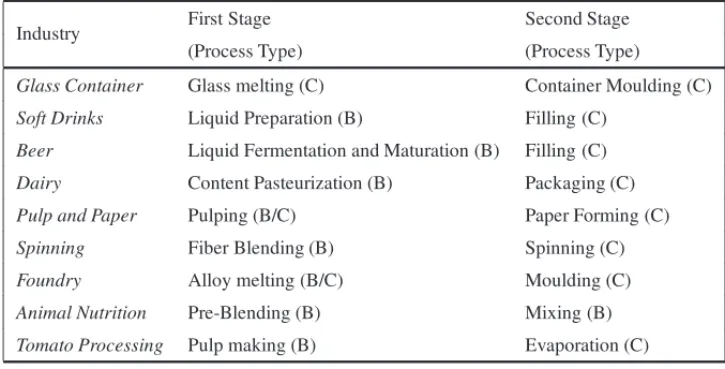
Process industries are businesses that add value to materials by mixing, separating, forming or chemical reactions. Processes may either be continuous (C) or batch (B), and generally require a rigid process control and high capital investment.
discrete, but are produced in very large quantities and therefore are not differentiated individually (Fransoo & Rutten, 1994).
Table 1–Production stages in different industrial environments.
Industry First Stage Second Stage
(Process Type) (Process Type)
Glass Container Glass melting (C) Container Moulding (C)
Soft Drinks Liquid Preparation (B) Filling (C)
Beer Liquid Fermentation and Maturation (B) Filling (C)
Dairy Content Pasteurization (B) Packaging (C)
Pulp and Paper Pulping (B/C) Paper Forming (C)
Spinning Fiber Blending (B) Spinning (C)
Foundry Alloy melting (B/C) Moulding (C)
Animal Nutrition Pre-Blending (B) Mixing (B)
Tomato Processing Pulp making (B) Evaporation (C)
Figure 1–Two-stage production environment of the spinning industry.
3 LOT SIZING AND SCHEDULING MODELS
The generic model considers the dynamic lot sizing and scheduling processes with a discrete time representation, in which the real-world decisions and events that occur continuously have to be translated into decisions and events occurring according to the discrete time scale. The objective is to minimize the total expenditure in inventory and setups to meet demand over a finite planning horizonT divided into a number of time periods. A plan simultaneously defines for every time period the production quantities and sequences forNproducts on a set of parallel capacitated machines. The beginning and ending of production lots are confined to the grid of the time periods. Without loss of generality, the single machine setting is considered in all the models presented in this paper. (External) demand is usually assumed to be known from forecasts and is to be met without backlog at the end of each time bucket. Sequencing decisions are introduced since both the setup times and costs are dependent on the production sequence.
There are two main types of models: big bucket and small bucket. In the former, the planning horizon is partitioned into a small number of lengthy time periods, and several products/setups may be produced/performed per period and machine. Such a period typically represents a time slot of one week or one month (also known as macro-periods). The Capacitated Lot Sizing Prob-lem with sequence-dependent setups (CLSD), which is an extension of the original Capacitated Lot Sizing Problem (CLSP), fits into this category. On the other hand, in small-bucket models, the planning horizon is divided into many short periods (such as days, shifts or hours) – usually referred to micro-periods, in which at most one setup may be performed. Therefore, depending on the models, we are limited to producing a maximum of one or two different products per period. Such models are useful for developing short-term production schedules. Lot-sizing and scheduling decisions are taken simultaneously since here a lot consists of producing the same item over one or more consecutive micro-periods. This is the case of the General Lotsizing and Scheduling Problem (GLSP).
Both CLSD and GLSP are chosen as they are the most studied models of each bucket-type. Their basic formulations are provided below. Both models incorporate common indices and parameters, as follows:
Sets and indices
i,j products,i,j =1, . . . ,N. t time periods,t=1, . . . ,T. Data
dit demand of productiin periodt(units) hit holding cost of one unit of productiin periodt capt machine capacity in periodt(time)
bit upper bound on production quantity of productiin periodt mi minimum lot sizes of producti
sti j time required to perform a changeover from producti to product j sci j cost incurred when performing a changeover from productito product j ¯
si start-up cost for producti
In order to capture the lot sizes and the resulting inventory the following decision variables are required:
Iit stock of productiat the end of periodt Xit quantity of productito be produced in periodt
3.1 Capacitated Lot sizing with sequence-dependent setups
As previously mentioned, the CLSD is considered a big-bucket problem, because several setups may be performed per period. To formulate the basic form of the CLSD problem consider the following additional decision variables to be optimized:
Zbit (=1) if the machine is set up for producti at the beginning of periodt Zeit (=1) if the machine is set up for producti at the end of periodt
Ti j t (=1) if a changeover from productito product j is performed in periodt.
As previously mentioned, the single machine case is presented here. The mixed integer mathe-matical formulation (MIP) for the basic CLSD reads:
min
i,t
hit ·Iit+
t,i,j
sci j·Ti j t+
i,t ¯
si·Zitb (1)
s.t. Ii,t−1+Xit =dit +Iit ∀i,t, (2)
i
pi·Xit+
i,j
sti j ·Ti j t ≤capt ∀t, (3)
Xit ≤bit· ⎛
⎝
j
Tj it +Zitb ⎞
⎠ ∀i,t, (4)
i
Zitb =1 ∀t, (5)
i
Zite =1 ∀t, (6)
Zbit+ j
Tj it =
j
{(i,j):Ti j t >0}does not include disconnected subtours ∀t. (8)
X, I ≥0, Z,T ∈ {0,1}. (9)
The objective function (1) minimizes the sum of holding, setup and start-up costs. It is assumed that production costs are product and time independent and therefore are not included in ex-pression (1). Nevertheless, such extension can be easily incorporated. The demand balancing constraints are described by constraints (2). Production time together with the time lost in setup operations should not exceed the capacity usually available (3). Constraints (4) link production quantities to the machine setup state: production may only occur if a setup is performed in the same period or the product is scheduled to be the first in the period. Constraints (5) and (6) ensure that the machine is set up for a single product in the beginning and at the end of each time period, while constraints (7) keep trace of each machine configuration, balancing the flow of setups as follows. If there are no setups in periodt the machine configuration at the end of the period is the same as in the beginning. If at least one setup is performed, three cases may appear for each producti: (i) more input than output setups, (ii) more output than input setups and (iii) equal number of input and output setups. In the first case the machine has to be set up for producti at the end of the period (Zite =1). The opposite scenario, the second case, forces the initial set up state for producti(Zitb =1). The third case happens when the product is neither the first nor the last in the sequence, or it is not part of the production sequence of the machine in that pe-riod. Note that the current model assumes a complete setup state loss between two time periods, assigning a start-up cost to the first item produced in each period. The domain of variables is defined in constraints (9).
Finally, constraints (8) prevent disconnected subtours, that is, sequences that start and end at the same setup state as long as this setup is not the first. These disconnected subtour elimination constraints are required to ensure the connectivity of the subgraph induced by the setup variables. A similar modelling trick is known in the context of travelling salesman problem. Guimar˜aes et al. (2014) have shown in their study that the CLSD modeling efficiency is directly linked to the selection of the proper subtour elimination constraints.
3.2 The General Lotsizing and Scheduling Problem
In the GLSP, each macro-period of the planning horizon is sub-divided into a number of micro-periods in which only one product can be produced. Therefore, the production sequence “comes for free”. In order to gain more flexibility, the lengths of the micro-periods are variable and determined by the production quantities. To formulate the GLSP model it is necessary to define the following additional variables:
Qis quantity of productiproduced in micro-periods,
Yis =1 if the machine is set up for producti in micro-periods,
Additionally, letAt = {ft, . . . ,lt}be the set of micro-periodssbelonging to time periodt, where ft (lt) refers to the first(last) micro-period of macro-periodt. The expression (lt− ft +1) gives the maximum number of lots allowed in time periodt. The GLSP model is as follows:
GLSP min
i,t
hit ·Iit +
i,j,s
sci j ·Zi j s (10)
s.t. Ii,t−1+
s∈At
Qis =dit+Iit ∀i,t, (11)
i,s∈At
pit·Qis +
i,j,s∈At
sti j ·Zi j s ≤capt ∀t, (12)
Qis ≤bit·Yis ∀i,t,s∈ At, (13)
i
Yis =1 ∀s, (14)
Zi j s ≥Yi,s−1+Yj s−1 ∀i, j,s, (15)
Qis ≥mi·Yis−Yi,s−1 ∀i,s, (16)
Q, I, Z ≥0, Y ∈ {0,1}. (17)
Equivalent to the CLSD, the objective function (10) of the GLSP aims at minimizing holding and setup costs. Demand in a given period is to be met from initial inventory or production within the current period, as stated by constraints (11). The production amounts of each product in a given period are derived from production in the different micro-periods/slots. Available capacity is consumed by production and setup times, as expressed by inequalities (12). The appropriate configuration of the machine to produce in any slot is guaranteed by constraints (13), while (14) enforce a single setup state per micro-period. Constraints (15) trace changeovers throughout the planning horizon, which occur at the beginning of the micro-period. Minimum lotsizes are intro-duced by constraints (16) to prevent phantom slots. Such scenario, which leads to an incorrect evaluation of setup times, will be discussed in the following section.
Figure 2 illustrates two solutions for the same instances of CLSD and GLSP. It is assumed that the start-up times are negligible or occur in between time periods (for instance, during night shifts or weekends). Note that both solutions are equivalent and comprise the same production plan. It entails three productions and two setups. For instance, in the first period, there are two production lots (products 1 and 2) and one setup (from product 1 to 2). The model formulations are translated as follows:
CLSD T1,2,1 =1, X1,1andX2,1are positive. Moreover, the machine is set up to product 2 at the end of period 1 (Ze2,1=1).
slot is used to set up the machine to product 2 (Z1,2,3 = 1) and to produce product 2 (Q2,3 = X2,1). In period 2 there is an idle micro-period (s = 6), with null production quantity. In fact, the lot production quantity of product 2 could be distributed arbitrarily among the micro-periods of period 2 without changing the actual schedule and the objec-tive function value (as scj j = 0, representing a phantom setup). There are well-known constraints (Fleischmann & Meyr, 1997) to avoid such redundancy and reduce the solu-tion space.
2
1 2 2
CLSD
3
1 2 2 2 3
1
t = 1 t = 2 t = 3
GLSP
2 3
s = 1 s = 2 s=3 s = 4 s = 5 s = 7 s = 8 s = 9
Setup
Figure 2–Illustrative example of a production plan.
4 MODELING SETUP OPERATIONS
Switching between production lots of two different products triggers operations, such as machine adjustments and cleansing. These setup operations, which are dependent on the sequence, con-sume scarce production time and may cause additional costs due to, for example, losses in raw materials or intermediate products and equipment wear. Correctly modeling these operations strongly depends on industrial features. We address below the features: a) setup conservation between time periods; b) period-overlapping setups; c) non-triangular setups; d) pre-defined production sequences and e) family setups.
a. Setup conservation between time periods.In some cases, the last machine setup state has to be carried over from one period to the next in order to properly account for the incurred setups. For instance, in process industries working on a 24×7 basis the borders in between periods simply appear for modeling reasons, since no physical separation exists (note that the process is continuous). In other situations, even if the machine gets idle (no production takes place), the setup state might have to be preserved (to correctly account for the setups). Figure 3 depicts a production plan from the soft-drink industry. The configuration of the machine toSodais carried from period 2 to period 3.
lot in the period. By introducing this extension we are not only improving solutions by decreasing the total setup cost but also contributing to creating feasible solutions in in-dustries that face considerable setup times. To introduce this change,Zeit = Zbi,t+1,∀i,t ands¯i =0,∀i(Almada-Lobo et al., 2007) are imposed. In Figure 3,ZeSoda,2 =ZbSoda,3. Note that the setup state is always preserved over idle periods (no shutdown occurs).
GLSP The setup carryover feature “comes for free” with the GLSP model (10)–(17). Addition-ally, after idle periods the machine remains set up for the item produced last. There are other cases where setup costs appear when there is no production over a certain time inter-val. This setting – the so-called loss of setup state (Fleischmann & Meyr, 1997) – can be modelled by introducing a dummy producti =0 to indicate a neutral setup state during idle periods. sc0i refers to the start-up costs incurred to set up the machine to producti after the no-production period.
t = 1 t = 2 t = 3
Orange juice Sparkling
drink Soda Soda
Figure 3–Period overlapping setup and carryover from soft-drink industrial setting.
b. Period-overlapping setups. It allows a continuous process starting and ending anywhere within the planning horizon, not only within the time period boundaries, thus overcoming this discrete time scheme limitation – see Figure 3. In the basic models setups have to be performed entirely within a (macro-)time period. This limitation is driven by the bucket orientation of dis-crete time models. In extremely tight capacity industries or whenever setups are substantially large when compared to the planning period length considering setup carryover may not be enough to provide feasible production plans. For instance, a color changeover in a furnace of a glass container manufacturer may take up to 3 days. In these scenarios allowing setups to over-lap the boundaries of periods forces them to be divided into two or more time periods. If two periods are enough, a setup is partially performed in periodt and concluded in periodt +1, which may deliver feasible valuable solutions in practice. This extension is calledsetup cross-over.
GLSP Here, by default setups are confined to take place within one micro-period. Despite their variable length, each micro-period belongs to a certain macro-period. Introducing period-overlapping setups into GLSP is not straightforward. One could adapt the mod-elling trick of CLSD. Another possibility would be considering micro-periods (slots) of arbitrary lengths again, without taking into consideration the time grid. This means that a slot would not be confined to one period, but could rather cover more periods (see Camargo et al., 2012).
In the soft drink industry example of Figure 3, the setup toSparkling drinkfromOrange juice starts in period 1 and is crossed over to period 2 (BOrange,S parkli ng,1 =1 in CLSD).
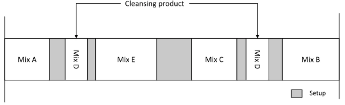
c. Non-triangular setups. In most production environments it is more efficient to change directly between two products than via a third product. This implies that in any optimal solution there is at most one production run for each product per time period. Under these conditions setups are said to obey the triangle inequality. Nevertheless, in some cases contamination occurs when changing from one product to another forcing additional cleansing operations. If a “cleans-ing” or shortcut product (often of lower grade) exists, contamination can be absorbed while pro-ducing such a product. Replacing the cleansing operations by a propro-ducing run often leads to the emmergence ofnon-triangular setups. In the presence of non-triangular setups, models have to allow for more than one production lot of each product per time period as it potentially re-duces setup times and costs. For example, in the animal nutrition industry contamination can occur in specific recipes (Clark et al., 2010). Here, the blending equipment must be cleaned in order to avoid contamination, resulting in substantial setups that require scarce production time. Fortunately, the amount of cleaning can be minimized by effectively sequencing production lots (Clark et al., 2014). Figure 4 depicts a typical plan from the animal feed supplements indus-try. Certain intermediate “cleansing” or shortcut products can cause non-triangular setup times. Producing productMix D– can be a wheat mixture – helps cleansing the machine (first after Mix Ais produced and then afterMix C), contributing to the reduction of overall setup times.
Mix A
Mix
D Mix E Mix C
Mix
D Mix B
Setup
Cleansing product
Figure 4–Production plan for a non-triangular setup instance of the animal feed supplements industry.
GLSP There is no need to adapt the standard GLSP to address the non-triangular requirement. As at most one setup can be performed in each micro-period, the production sequence is implicitly defined from the production lots. Therefore, in GLSP constraints that cut off disconnected subtours do not have to be considered. Note that the number of micro-periods per macro-period imposes an upper bound on the number production runs, and therefore should be large enough to allow for multiple setups of the same product.
Under these circumstances, a minimum lot size has to be imposed in order to eliminate unac-ceptable contamination or due to a modeling necessity to avoid fictitious setups to the shortcut product (as they would reduce setup time and cost). As the production run may overlap more than one period (allowed by means of setup carryover), the calculation of the size of the lots must take into account runs that pass over contiguous periods.
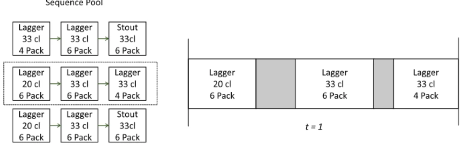
d. Pre-defined production sequences. The motivation for this feature may come from the modeling and industrial perspectives. In the former, whenever the set of products to be produced becomes relatively large, the model tends to be intractable due to the number of variables. The latter, in some industrial applications, requires the sequence to be fixeda priorifor technological, costs or marketing reasons. A modeling alternative is to reformulate the production scheduling by selecting feasible production sequences (Haase & Kimms, 2000). Consider the set of products presented in Figure 5 from the beer industry: {Lagger 20cl 6Pack; Lagger 33cl 4Pack; Lagger 33cl 6Pack; Stout 33cl 6Pack}. The pool of sequences has been defineda prioribased on different criteria: same pack size, same volume, same beer. The second sequence was selected for time period 1. Note that the number of sequences per period is variable and the number of products per sequence does not need to be the same.
Lagger 20 cl 6 Pack Lagger 33 cl 6 Pack Lagger 33 cl 4 Pack Lagger 33 cl 6 Pack Lagger 33 cl 4 Pack Stout 33cl 6 Pack Lagger 20 cl 6 Pack Lagger 33 cl 4 Pack Lagger 33 cl 6 Pack Lagger 20 cl 6 Pack Lagger 33 cl 6 Pack Stout 33cl 6 Pack Sequence Pool
t = 1
Figure 5–Selection of a sequence from a pool for the beer industry.
The set Seqt of all feasible production sequences must be defined to schedule products on the machine in periodt, indexed bys′ =1, . . . ,|Seqt|. Binary decision variablesWt s′ capture whether sequences′is chosen in periodt, whereas parameterseis′ make the link between the product and the sequence, defining whether the machine is ever set up for producti in sequences′.
GLSP While pre-defined sequences may significantly reduce the complexity of the CLSD, it is not the case for the GLSP as by default there is no need to include the complicated subtour elimination constraints. Sequences are hereby selected per micro-period (instead of period for CLSD). Only one sequence can be allocated to each micro-period.
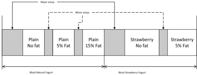
e. Family setups. In some industrial settings, there are important scale differences between the setups performed. Products are grouped into families implying that a changeover between products of the same family is much less costly than a changeover between products of different families. Changing between product families is often referred asjointormajor setup; chang-ing between items of the same family is known asminor setup. Another important difference can be associated with the setup structure, as sequence dependent setups may only apply when changing between families and sequence independent setups are present when changing between items of the same family. This scenario is closely related to the concept of recipe often found in fast moving consumer food goods (which works under a make & pack system). Changing between recipes requires major setups related to cleansing, while changing between items of the same recipe requires minor setups. Recipe related setups are more significant than tuning the size/format of packing devices.
To model these production contexts it is possible to adapt the block planning formulation (G¨unther et al., 2006) where each block is a recipe, and the sequence of products is seta pri-oriinside each recipe. Figure 6 depicts a production schedule from the dairy industry with two blocks,Plain YogurtandStrawberry Yogurt. A major setup occurs between the recipes/blocks due to the need to cleanse the lines and link the packaging lines to the new yoghurt tank. The sequence of products in each block is seta prioridue to natural constraints in this kind of indus-try (increasing percentage of fat).
Plain No fat
Plain 5% Fat
Plain 15% Fat
Strawberry No fat
Strawberry 5% Fat Major setup
Minor setup
Block Natural Yogurt Block Strawberry Yogurt
CLSD Ti j t setup variables have to be redefined and only applied to the changeovers between families. New sequence independent setup variables need to be introduced for the product level.
GLSP Zi j s setup variables refer now to the changeover between families/blocks. One block is scheduled in each micro-period. The time to set up the block and the amount of items produced that belong to the block determines the length of the micro-period.
5 SYNCHRONIZATION OF RESOURCES
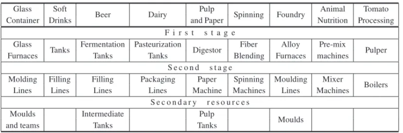
Synchronizing resources may be critical at operational level, where plans need to be more de-tailed. This is particularly important in the presence of shifting bottlenecks or when the schedule of a resource may impact the overall production costs. This can be the case of multi-stage pro-duction environments, where it is mandatory to synchronize the flow between the stages, and also when there are secondary scarce resources. Table 2 depicts the different resources to be synchronized for the subset of process industries mentioned before.
Table 2–Production stages and secondary resources in different industrial environments.
Glass Soft
Beer Dairy Pulp Spinning Foundry Animal Tomato
Container Drinks and Paper Nutrition Processing
F i r s t s t a g e Glass
Tanks Fermentation Pasteurization Digestor Fiber Alloy Pre-mix Pulper
Furnaces Tanks Tanks Blending Furnaces machines
S e c o n d s t a g e
Molding Filling Filling Packaging Paper Spinning Moulding Mixer
Boilers
Lines Lines Lines Lines Machine Machines Lines Machines
S e c o n d a r y r e s o u r c e s
Moulds Intermediate Pulp
Moulds
and teams Tanks Tanks
The impact of batch versus continuous processes, and the presence of scarce resources from a modelling point-of-view will be discussed below. Afterwards, an analysis is provided on how the flexibility given by variable (controllable) production rates of the resources and by intermediate buffers can be incorporated in the models.
a. Batch vs. continuous processes. When considering more than one production stage, it is important to take into account the way process material flows across production resources. As previously mentioned, resources may operate in batches or continuously. Two examples are presented below to illustrate the impact of the different flows in L&S.
prepared, because it is necessary to clean the tank and mix the ingredients). The syrup can only be sent to filling machines (in the second stage, where it is bottled) after its preparation process is fully completed. In case the necessary flavor is not ready, the filling machines must wait for its preparation to guarantee a correct synchronization between both stages.
With regard to continuous processes, the case of the glass container industry is highlighted next. Furnaces produce glass paste that is distributed continuously to a set of molding machines that form the container. Figure 7 presents a production environment with one furnace that feeds two molding machines (M1 and M2). The furnace can only melt one color at a time and, con-sequently, all machines attached to it produce containers of the same color. The Emerald Green (EG) color glass is the first campaign. Products EG1 to EG4 are of the same color EG. During a product changeover in a machine, the furnace keeps feeding the machine, however, the (glass) gobs are discarded and melted down again in the furnace. During the color changeover in the furnace from EG to AM (amber), the associated machines may stop producing (in case the in-termediate glass is of no value). The association between the flow in both stages needs to be properly handled by the models, as will be seen later.
EG1 AM2
Machine Setup
Glass EG Glass AM
EG3 AM4
Furnace
M1
M2
EG2
EG4
Machine Waiting Time Furnace Setup
Setup Operator
t = 1
s = 1 s = 5 s = 7
Figure 7–Synchronizing setup operators and production stages in glass container industry.
To explicitly model synchronization issues triggered by the type of material flow between stages, and because scarce resources need to be scheduled, it is necessary to capture the precise timing of events (any resource state modification), and therefore incorporate a continuous time axis within the discrete time scheme.
CLSD It can be adapted to link the beginning and the end of the usage of each resource in each stage. Variablesµbkt andµekt are added to explicitly trace the beginning and the end of the event related to a given resource to a machine at each period, respectively. It is possible to observe that here the concept of resourcekis wide, and may refer to the color of glass being produced (AM or EG) or to the setup operator’s activities. For some type of scarce resources, decision variablesWt mm′kmay help to indicate whether resourcekis used on machinemafter being used on machinem′in periodt. In Figure 7,W1,2,1,1 = 1. Nevertheless, when different intra-period events have to be captured, it may be very difficult to incorporate various constraints related to the synchronization of resources in the CLSD. In the same example, tracing another event of the setup operator on M1 or M2 is not straightforward.
GLSP It can be easily adapted assuming that at most one resource state modification may take place per micro-period, and that the length for each micro-period is used across all ma-chines and stages (that is, a common time grid). This feature makes synchronization be-tween resources easier, and considers more realistic flows bebe-tween stages (specially in batch production, where additional requirements may emerge as in the case of pulp and paper (P&P) – Figueira et al., 2013). Variablesµbs andµes are necessary to define the start-ing and endstart-ing times of micro-periods. The drawback is the computationally efficiency, as the number of micro-periods to decidea priorihas to be large enough not to cut off optimal solutions. In Figure 7 at least seven micro-periods are necessary to generate the depicted plan.
c. Intermediate buffers. Production stages can be connected directly or have intermediate buffers in between. If they are connected directly, it is necessary to know exactly when the production of each item starts in the second stage, so that it can be synchronized with the material produced in the first stage (see Camargo et al., 2012). When an intermediate buffer exists, the mass balances need to be evaluated whenever a changeover occurs (as different products will consume the input material at different rates), in order to ensure that the buffer limits are never violated.
CLSD Constraints (2) need to be extended (to consider mass balances or intermediate products).
GLSP Constraints (11) need to be extended. Once again, small-bucket models are more flexible for this purpose than big-bucket models.
resources at specific points in time may help to coordinate different stages and resources, espe-cially in environments with shifting bottlenecks. Figure 8 provides an example from the P&P industry (for further details, readers are referred to Figueira et al., 2015). Here, raw materials are first processed and converted into pulp in the digester. The virgin pulp is stocked in silos (inter-mediate buffer), waiting to be pulled from the paper machine where paper products (of different grades) are produced. The goal is to maximize the throughput of the mill. As the bottleneck is non-stationary (shifting from the digester to the pulp tanks to the paper machine), it is necessary to define in each point in time the production rate of the most critical resource, which is the digester. When the machine is producing higher grade paper, even when the digester is at maxi-mum speed, the pulp levels in the tanks decrease. Contrarily, during lower-grade campaigns the output of the digester typically exceeds the amount that needs to be processed, therefore allowing the silos to recover the stock (the rate of the digester is reduced).
Figure 8–Intermediate virgin pulp buffer and digester’s variable throughput in the P&P.
CLSD Considering various production rate changeovers within the same (macro-)period with-out discritisizing the period is not straightforward. We are not aware of any publication addressing it. Note that average production rates per period constrains the solution space. On the other hand, speed changes between time periods are easy to handle.
GLSP This feature may require production rates to be modeled explicitly or just implicitly. In the latter the production quantity is constrained by the maximum and/or minimum rates. The former uses a variable to explicitly model the production rate. This is required for instance in the case where production rates are limited to a maximum change. Often these rates must also be as steady as possible and thus changes in rates should be minimized in the objective function. Nevertheless, an explicit variable for production rates can make the model non-linear (from the need to multiply rates by slot lengths). In that case, the model should be linearized by using a discrete grid of rates or by leaving the rates smoothness to a post-optimization phase. For instance, an additional binary variableYsdigv , equaling 1
6 PRODUCTS’ FEATURES
The properties of some products may also require changes in the model to fit reality.
a. Perishability. One of the most relevant features is perishability. Not accounting for product deterioration over time and/or shelf life can lead to significant spoilage costs. In practice it is necessary to trace the age of inventory over the planning horizon. The simple plant location (SPL) reformulation can be used to capture this age-dependent inventory. The new production decision variables simultaneously define the production and consumption periods, thus making it possible to capture the age of inventory. This extension not only makes it possible to limit the use of stock during shelf life, but also to model delivery freshness and spoilage amounts, which are key features in the dairy industry (for example, Amorim et al., 2013).
CLSD Decision variables Xit are replaced byXextit t′, which define the fraction of demand for producti in periodt′that is produced in periodt. Some families of constraints (related to production) need to be adapted.
GLSP The age of inventory is only tracked on a macro-period basis. Therefore, variablesXextit t′ are added to the model as in CLSD.
b. Manufacturing constraints. Products’ manufacturing constraints can also impact modeling decisions. These constraints may impose bounds for certain products in minimum, maximum or fixed size production runs, and can emerge from multiple reasons: quality assurance, materi-als consumptions, capacity of resources and utilization, and production already released. In the presence of setup carryover production runs can be split in two periods, and therefore additional lot size constraints must address this issue properly (see e.g. Figueira et al., 2015).
CLSD When considering a fixed production run size, besides eliminating theXitvariables from the formulation since the number of setups automatically define the production quantity, multiple production runs for the same product can also occur in the optimal solution. Thus, this extra requirement leads to formulations close to the ones considered for the case of non-triangular setups.
GLSP Because just one run occurs per micro-period, incorporating additional manufacturing constraints is a straightforward process.
7 PLANNING PROCESS
as new information on demand forecasts/orders is available, together with the data coming from the execution of previous plans. This section briefly addresses a few features that should guide the planning process, namely the rolling horizon approach and the underlying key performance indicators (KPIs). No distinction will be made here between CLSD and GLSP, as the majority of these requirements impose adaptations on a (macro-)period structure level.
a. Rolling horizon.Much of the research on lot sizing and scheduling problems has just taken into consideration the optimization of their static version. Better solutions are usually applied on a rolling horizon approach (Araujo & Clark, 2013). Moreover, in practice, planners try to follow this scheme (even if not in a systematic way) to avoid the myopic nature of the static variants (especially in between two planning horizons). The basic idea is to create a plan for a specific planning horizon, but only the first period(s) is(are) executed. The remaining periods can be relaxed (for instance, not sequencing the production lots within each period) as they are re-optimized and updated as the horizon is rolled forward and new data is available. A few key parameters influence the success of the rolling horizon approach, such as the planning horizon length, the planning frequency, the number of frozen periods and the way the decision variables are frozen (for example, fixing setup-related variables and/or quantities). There is naturally a trade-off between the flexibility, cost and stability/nervousness of the plans.
With regards to the KPIs that drive the planning process, the standard goal is to maximize met demand in the most cost-effective manner. The idea is to get the best trade-off between setup costs and holding costs under tight capacities. Notwithstanding, other KPIs may emerge in dif-ferent applications.
b. Demand satisfaction related costs. Demand for individual products is aggregated per time period, and comes from actual orders placed or forecasting systems. In case unmet demand is allowed, costs related to backlog or to lost sales are usually considered in deterministic lot sizing and scheduling (Araujo et al., 2007). Note that in stochastic variants – not covered here – cus-tomer service related measures are explicitly incorporated (e.g. Ramezanian & Saidi-Mehrabad, 2013). In some practical applications, companies can not backlog for more than one planning period, and the respective demand is converted into lost sales. In the case of perishable goods, it is necessary to incorporate discarding costs. Spoilage costs, incurred whenever stock is held be-yond the product’s shelf-life, are usually defined as opportunity costs coming from the potential revenue yielded by the product to be discarded.
d. Production related costs. The trade-off between setup and holding costs is sometimes ex-tended to production costs. This is especially relevant in the presence of an heterogeneous multi-machine environment per production stage (for instance, multi-machines with different technologies and processing rates). In capital intensive industries the main operational driver is to maximize the facilities throughput (for example, the glass tonnage produced in furnaces in the glass con-tainer industry and steam produced in the pulp and paper industry in Almada-Lobo et al., 2010 and Furlan et al., 2015, respectively). In other cases, in order to promote the steadiness of the production resources, it is necessary to minimize the variation of the respective processing rates along the planning horizon.
e. Stock related costs.Stock holding costs, which may be time and product dependent, penalize the production in advance that companies do to cope with scarce capacity. Stocks of interme-diate or final products are differentiated according to the underlying bill-of-materials. In some industrial applications, guaranteing the right balance of attributes of the intermediate products in inventory is as important as minimizing the stock carried at a certain point in time. For in-stance, in the spinning industry, the right combination of different fiber attributes is mandatory to achieve a homogeneous blend. Here, it is necessary to minimize the variation of quality attributes between two consecutive fiber blends (Camargo et al., 2015).
8 DISCUSSION
B
E
RNA
RDO
A
L
M
A
D
A
-L
O
B
O
e
t
a
l.
Table 3–Modeling L&S features in different industrial settings.
Class Features Glass Container Soft Drinks Beer Dairy
Setups
Carryover x x x Crossover x x
Non-triangular
Pre-defined sequences x x Family Setups x x x x
Resources
Interm. Buffers x x x Scarce Resources x
Variable Prod. Rates
Synchron. Between stages x x
Product Perishability x Lot sizes x x
Models CLSD-type GLSP-type
Almada-Lobo et al., 2007 Almada-Lobo et al., 2010
Maldonado et al., 2014 Ferreira et al., 2012 Ferreira et al., 2009 Ferreira et al., 2012 Toledo et al., 2014
Kopanos et al., 2011 Guimar˜aes et al., 2013
Baldo et al., 2014
Kopanos et al., 2011 Marinelli et al., 2007 Amorim et al., 2011
a
O
per
ac
ional,
V
ol.
35(
3)
,
INDUS T R IA L INS IG HT S INT O L O T S IZ ING A N D S CHE DUL ING M O D E L ING
Table 3 (continuation) –Modeling L&S features in different industrial settings.
Class Features Pulp & Paper Spinning Foundry Animal Nutrition Tomato Proc.
Setups
Carryover x x x
Crossover
Non-triangular x
Pre-defined sequences x
Family Setups
Resources
Interm. Buffers x x x
Scarce Resources
Variable Prod. Rates x
Synchron. Between stages x x
Product Perishability
Lot sizes x
Models CLSD-type GLSP-type
Santos and
Almada-Lobo, 2012
Furlan et al., 2015
Camargo et al., 2014
Araujo and Clark, 2013
Araujo et al., 2007
Araujo et al., 2008
Clark et al., 2010
Clark et al., 2014
Toso et al., 2009
The difficulty of incorporating practical requirements depends on the feature to be modelled and on the underlying model. A few applications assume one stationary bottleneck stage. Therefore, only one production stage is explicitly addressed in the model. When the scheduling of both stages needs to be synchronized, GLSP has been the chosen model by researchers. To the best of our knowledge, in short-term L&S, there is no research on CLSD with this feature. The same situation occurs with variable production rates. Morevoer, it seems that significant setup times are a critical issue for the GLSP-type of models with regard to the length of the microperiod.
From Table 3 it is also possible to observe that the community has been quite active in incorporat-ing more complex setup patterns within the models (which naturally comes from the significant setups that characterize those industries). Nevertheless, there are still numerous areas for poten-tial future research. The level of detail on the usage of the resources still has a long way to go. The synchronization between stages needs further work especially in the presence of lead times. This can boost the use of these models in more complex production environments, including those where it is crucial to define the processing times of the resources. In fact, for simplicity reasons, researchers have assumed constant production rates. In order to maximize the through-put, it is important to incorporate the speeds in the set of decision variables to be taken. Intro-ducing uncertainty is also another promising field of future research (e.g. [32]). Despite their operational/tactical nature, many of the model parameters are likely to suffer from variations when executing the plans in practice. Understanding the effects of such variability can help man-agers in their daily planning activities. Industrial applications of stochastic L&S have not been published. Finally, integrating lot sizing and scheduling with other supply chain related problems (especially demand planning) can further leverage the effective use of the tight capacity.
ACKNOWLEDGMENTS
This work is partially funded by the ERDF – European Regional Development Fund through the COMPETE Programme (operational programme for competitiveness) and by National Funds through the FCT – Fundac¸˜ao para a Ciˆencia e a Tecnologia (Portuguese Foundation for Science and Technology) within project “FCOMP-01-0124-FEDER-037281”.
REFERENCES
[1] ALMADA-LOBOB, KLABJAND, OLIVEIRAJF & CARRAVILLAMA. 2007. Single machine multi-product capacitated lot sizing with sequence-dependent setups.International Journal of Production Research,45(20): 4873–4894.
[2] ALMADA-LOBOB, KLABJAND, CARRAVILLAMAANDOLIVEIRAJF. 2010. Multiple machine continuous setup lotsizing with sequence-dependent setups.Computational Optimization and Appli-cations,47(3): 529–552.
[4] AMORIMP, ANTUNESCH & ALMADA-LOBOB. 2011. Multi-objective lot-sizing and scheduling dealing with perishability issues.Industrial & Engineering Chemistry Research,50(6): 3371–3381.
[5] AMORIMP, COSTAAM & ALMADA-LOBOB. 2013. Influence of consumer purchasing behaviour on the production planning of perishable food.OR Spectrum,36(3): 669–692.
[6] ARAUJO SA & CLARKA. 2013. A priori reformulations for joint rolling-horizon scheduling of materials processing and lot-sizing problem.Computers and Industrial Engineering,65(4): 577–585.
[7] ARAUJOSA, ARENALESM & CLARKA. 2007. Joint rolling-horizon scheduling of materials pro-cessing and lot-sizing with sequence-dependent setups.Journal of Heuristics,13(4): 337–358.
[8] ARAUJO SA, ARENALES MN & CLARKAR. 2008. Lot sizing and furnace scheduling in small foundries.Computers and Operations Research,35(3): 916–932. Part Special Issue: New Trends in Locational Analysis.
[9] BALDOTA, SANTOSMO, ALMADA-LOBOB & MORABITOR. 2014. An optimization approach for the lot sizing and scheduling problem in the brewery industry.Computers and Industrial Engi-neering,72: 58–71.
[10] BOONMEEA & SETHANANK. 2015. A glnpso for multi-level capacitated lot-sizing and schedul-ing problem in the poultry industry.European Journal of Operational Research, in press, 2015. 10.1590/0101-7438.2015.035.03.0439http://dx.doi.org/10.1016/j.ejor.2015.09.020.
[11] CAMARGOVC, TOLEDO FM & ALMADA-LOBO B. 2014. Hops – hamming-oriented partition search for production planning in the spinning industry.European Journal of Operational Research,
234(1): 266–277.
[12] CAMARGOVCB, TOLEDOFMB & ALMADA-LOBOB. 2012. Three time-based scale formulations for the two-stage lot sizing and scheduling in process industries.Journal of the Operational Research Society,63(11): 1613–1630.
[13] CAMARGOVCB, ALMADA-LOBOB & TOLEDOFMB. 2015. Integrated lot-sizing, scheduling and blending decisions in the spinning industry.Working paper, University of S˜ao Paulo.
[14] CLARKA, MORABITOR & TOSOE. 2010. Production setup-sequencing and lot-sizing at an animal nutrition plant through atsp subtour elimination and patching.Journal of Scheduling,13(2): 111–121.
[15] CLARKA, ALMADA-LOBOB & ALMEDERC. 2011. Lot sizing and scheduling: industrial exten-sions and research opportunities.International Journal of Production Research,49(9): 2457–2461.
[16] CLARK A, MAHDIEH M & RANGEL S. 2014. Production lot sizing and scheduling with non-triangular sequence-dependent setup times.International Journal of Production Research, 52(8): 2490–2503.
[17] FERREIRAD, MORABITOR & RANGELS. 2009. Solution approaches for the soft drink integrated production lot sizing and scheduling problem.European Journal of Operational Research,196(2): 697–706.
[18] FERREIRAD, CLARKAR, ALMADA-LOBOB & MORABITOR. 2012. Single-stage formulations for synchronised two-stage lot sizing and scheduling in soft drink production.International Journal
of Production Economics,136(2): 255–265.
[20] FIGUEIRAG, AMORIMP, GUIMARAES˜ L, AMORIM-LOPESM, NEVES-MOREIRAF & ALMADA -LOBOB. 2015. A decision support system for the operational production planning and scheduling of an integrated pulp and paper mill.Computers & Chemical Engineering,77: 85–104.
[21] FLEISCHMANNB & MEYRH. 1997. The general lotsizing and scheduling problem.OR Spektrum,
19(1): 11–21.
[22] FLEISCHMANNB & MEYRH. 2003. Planning hierarchy, modeling and advanced planning systems. In S. Graves and A. de Kok, editors,Supply Chain Management: Design, Coordination and Opera-tion, volume 11 ofHandbooks in Operations Research and Management Science, pages 455 – 523. Elsevier.
[23] FRANSOOJC & RUTTENWG. 1994. A typology of production control situations in process indus-tries.International Journal of Operations & Production Managemen,14(12): 47–57.
[24] FURLANM, ALMADA-LOBOB, SANTOSM & MORABITOR. 2015. Unequal individual genetic algorithm with intelligent diversification for the lot-scheduling problem in integrated mills using multiple-paper machines.Computers and Operations Research,59: 33–50.
[25] GUIMARAES˜ L, KLABJAND & ALMADA-LOBOB. 2013. Pricing, relaxing and fixing under lot sizing and scheduling.European Journal of Operational Research,230(2): 399–411.
[26] GUIMARAES˜ L, KLABJAND & ALMADA-LOBOB. 2014. Modeling lotsizing and scheduling prob-lems with sequence dependent setups.European Journal of Operational Research,239(3): 644–662.
[27] G ¨UNTHERH-O, GRUNOWM & NEUHAUSU. 2006. Realizing block planning concepts in make-and-pack production using MILP modelling and SAP APO.International Journal of Production
Research,44(18-19): 3711–3726.
[28] HAASEK. 1996. Capacitated lot-sizing with sequence dependent setup costs.OR Spectrum,18(1): 51–59.
[29] HAASEK & KIMMSA. 2000. Lot sizing and scheduling with sequence-dependent setup costs and times and efficient rescheduling opportunities.International Journal of Production Economics,66(2): 159–169.
[30] KALLRATHJ. 2002. Planning and scheduling in the process industry.OR Spectrum,24(3): 219–250. [31] KOPANOSGM, PUIGJANERL & GEORGIADISMC. 2011. Production scheduling in multiproduct multistage semicontinuous food processes.Industrial & Engineering Chemistry Research,50(10): 6316–6324.
[32] L ¨OHNDORFN, RIELM & MINNERS. 2014. Simulation optimization for the stochastic economic lot scheduling problem with sequence-dependent setup times.International Journal of Production
Economics,157: 170–176.
[33] MALDONADOM, RANGELS & FERREIRAD. 2014. A study of different subsequence elimination strategies for the soft drink production planning.Journal of Applied Research and Technology,12(4): 631–641.
[34] MARINELLIF, NENNIM & SFORZAA. 2007. Capacitated lot sizing and scheduling with parallel machines and shared buffers: A case study in a packaging company.Annals of Operations Research,
[35] MENEZES A, CLARKA & ALMADA-LOBOB. 2011. Capacitated lot-sizing and scheduling with sequence-dependent, period-overlapping and non-triangular setups.Journal of Scheduling, 14(2): 209–219.
[36] MEYRH. 2002. Simultaneous lotsizing and scheduling on parallel machines.European Journal of
Operational Research,139(2): 277–292.
[37] MEYRH & MANNM. 2013. A decomposition approach for the general lotsizing and scheduling problem for parallel production lines.European Journal of Operational Research,229(3): 718–731.
[38] POCHETY. 2001. Mathematical programming models and formulations for deterministic production planning problems. InComputational Combinatorial Optimization, pages 57–111.
[39] RAMEZANIAN R & SAIDI-MEHRABAD M. 2013. Hybrid simulated annealing and mip-based heuristics for stochastic lot-sizing and scheduling problem in capacitated multi-stage production system.Applied Mathematical Modelling,37(7): 5134–5147.
[40] SANTOSMO & ALMADA-LOBOB. 2012. Integrated pulp and paper mill planning and scheduling. Computers and Industrial Engineering,63(1): 1–12.
[41] SEEANNERF & MEYRH. 2013. Multi-stage simultaneous lot-sizing and scheduling for flow line production.OR Spectrum,35(1): 33–73.
[42] TEMPELMEIERH & BUSCHKUHLL. 2008. Dynamic multi-machine lotsizing and sequencing with simultaneous scheduling of a common setup resource.International Journal of Production Eco-nomics,113(1): 401–412.
[43] TEMPELMEIER H & COPIL K. 2015. Capacitated lot sizing with parallel machines, sequence-dependent setups and a common setup operator.Accepted for publication in OR Spectrum.
[44] TOLEDOCFM,DEOLIVEIRAL,DEFREITASPEREIRAR, FRANC¸APM & MORABITOR. 2014. A genetic algorithm/mathematical programming approach to solve a two-level soft drink production problem.Computers and Operations Research,48: 40–52.