DOI: http://dx.doi.org/10.1590/1806-9126-RBEF-2018-0202 Licença Creative Commons
Simple but accurate periodic solutions for the nonlinear
pendulum equation
Fábio M. S. Lima
∗11Universidade de Brasilia, Instituto de Fisica, Brasilia, DF, Brasil
Received on July 08, 2018; Revised on July 18, 2018; Accepted on July 23, 2018.
Despite its elementary structure, the simple pendulum oscillations are described by a nonlinear differential equation whose exact solution for the angular displacement from vertical as a function of time cannot be expressed in terms of an elementary function, so either a numerical treatment or some analytical approximation is ultimately demanded. Such solutions have been thoroughly investigated due to the abundance of distinct pendular systems in nature and, more recently, due to the availability of automatic data acquisition systems in undergraduate laboratories. However, it is well-known that numerical solutions to differential equations usually loose accuracy (due to accumulation of roundoff errors) and polynomial approximations diverge after long time intervals. In this work, I take a few terms of the Fourier series expansion of the elliptic function sn(u;k) as a source of accurate
periodicsolutions for the pendulum equation. Interestingly, these approximations remain accurate for arbitrarily long time intervals, even for large amplitudes, which shows its adequacy for the analysis of experimental data gathered in classical mechanics classes.
Keywords:Simple pendulum, Nonlinear oscillations, Fourier series, Jacobi elliptic functions.
“For the simple pendulum does not naturally provide an accurate and equal measure of time, since its wider motions are observed to be slower than its narrower motions.”
C. Huygens,Horologium oscillatorium(1673)
1. Introduction
The simple pendulum is a prototype for the study of nonlinear systems and their stability [1]. In fact, pendu-lar oscillations arise in distinct fields of physical science and technology, e.g. acoustic vibrations [2], molecular oscillations [3], optically torqued nanorods [4], Joseph-son superconducting junctions [3, 5], elliptic filters in electronics [6], gravitational lensing [7], smetic C liquid crystals [8], advanced field theory [9], oscillations of build-ings in earthquakes [10], etc. In the small-angle regime, the approximation sinθ≈θ works and the equation of motion can be linearized, becoming solvable in terms of a sinusoidal function of time. Beyond this regime, the nonlinear nature of the pendulum motion becomes apparent: (i) the period increases with the amplitude; and (ii) the function θ(t) departs more and more from a harmonic behavior. In the nonlinear regime, the sim-plicity of the sinusoidal solution is lost and the equation of motion becomes unsolvable in terms of elementary functions, so either a direct numerical solution or some analytical approximation is demanded. However, numeri-cal solutions for the pendulum equation loose accuracy
for long time intervals due to the accumulation of round-off errors (inherent to numerical routines) [11], whereas polynomial approximations (including truncated Taylor series) have an intrinsic defect, namely the divergence for very long time intervals, as follows from the fact that limt→∞Pn(t) = ± ∞ for any polynomial with degree n >0. Here in this work, I show how these limitations can be circumvented by taking a few terms of the Fourier series expansion of the elliptic function sn(u;k) as the basis to build a simple periodicapproximation for θ(t) which is accurate for allt >0, even for amplitudes near πrad.
2. Equation of motion and exact solution
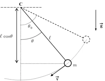
A simple pendulum consists of a small bob of mass m suspended by a weightless, thin rigid rod of length ℓ fixed at the upper end and free to rotate around the suspension point C, as indicated in Fig. 1. Its oscillatory motion can be studied by applying Newton’s second law of motion for rotations, which, in the absence of dissipative forces and taking the counterclockwise direction of motion as positive, readsFigure 1:The simple pendulum motion. At t= 0, it is released
at rest from a position that forms an angle 0< θ0< πrad with the vertical, then passing by an angleθ, for some 0< t < T /4,
with a scalar velocity v=ℓθ˙.
wheregis the local acceleration of gravity and I=m ℓ2
is the pendulum’s moment of inertia. This simplifies to thenonlinear pendulum equation [12, Sec. 4.4]:
¨ θ+ω2
sinθ= 0, (2)
where ω≡pg/ℓ.
In thesmall-angle regime |θ| ≪π/2rad the approx-imation sinθ ≈ θ works, which linearizes Eq. (2) to ¨
θ+ω2
θ= 0. For the usual initial conditions θ(0) =θ0
and θ˙(0) = 0, the solution is [12, Sec. 3.2]
θ(t) =θ0 cos (ωt), (3)
which reveals asimple harmonic motion whose period is T0 = 2π/ω = 2π
p
ℓ/g. As shown in Ref. [13], this formula is accurate to less than 0.5% for amplitudes below10◦. Then, in the small-angle regime the period is
practically independent of amplitudeθ0 (isochronism).
Beyond this regime, one should retake the nonlinear differential equation in Eq. (2). Alternatively, an expres-sion for the inverse function t(θ) can be derived for any 0 < θ0 < π rad from the conservation of mechanical
energy, without a deeper discussion on differential equa-tions [12–14]. On taking the zero level of the potential energy at the lowest point, one finds [13]
m g ℓ(1−cosθ0) =
1 2m ℓ
2 ˙
θ2
+m g ℓ(1−cosθ). (4)
On isolatingθ, one has˙
˙ θ=±
r
2g
ℓ (cosθ−cosθ0) , (5)
where the ‘+’ sign is for the counterclockwise motion and the ‘−’ sign is for the clockwise one. The integration
fromθ0 to any θ(t) with 0< t≤T /2 (hence using the
‘−’ sign) yields
t= √1 2 ω
Z θ0
θ
1 √
cosβ−cosθ0
dβ . (6)
This improper integral becomes a proper one making cosβ = 1−2 sin2
(β/2), followed by the substitution sin (β/2) =k sinφ, wherek≡sin(θ0/2). This yields
t= 1 ω
Z π/2
ϕ
1
p
1−k2sin2φdφ=
K(k)−u(ϕ;k)
ω , (7)
where sinϕ= sin (θ/2)/k,
K(k)≡
Z π/2
0
1
p
1−k2 sin2φ dφ (8)
is the complete elliptic integral of the first kind, and
u(ϕ;k)≡
Z ϕ
0
1
p
1−k2sin2
φ dφ (9)
is the incomplete one [15]. The parameterkis the elliptic modulusand ϕ= arcsin [sin(θ/2)/k] is theamplitude of u(ϕ;k). Though these integrals cannot be expressed in a closed-form in terms of elementary functions only [16], a formula for the exact pendulum periodT can be de-rived by taking t=T /4 and ϕ= 0 in Eq. (7), which corresponds to θ(T /4) = 0. This yields
T = 4 ω
Z π/2
0
1
p
1−k2sin2
φ dφ= 4 ω K(k)
= 2
π T0K(k), 0< k <1. (10) The computation of the exact period T then demands the numerical evaluation ofK(k), which is usually done via numerical integration or some recursive iterations in a computer [6]. Alternatively, one can use some of the practical approximate formulae available in literature (see, e.g., Refs. [17–20]). Anyway, Eq. (10) shows that the pendulum period increases from T0 to infinity as
the amplitude θ0 goes from 0to π, as expected since
the top vertical positionθ0=πis a point of (unstable)
equilibrium [14]. This increase ofT withθ0 makes the
harmonic solution in Eq. (3) inappropriate for large-angle oscillations.
Though the exact solution of Eq. (2), for any 0 < θ0< πrad, cannot be expressed as a finite combination
of elementary functions, it can be written in terms of elliptic functions, as proved independently by Abel and Jacobi in 1827 [21,22]. For a given k,k2<1, the three
basic Jacobi elliptic functions are defined as inverses of the elliptic integralu(ϕ;k)[15]:
sn(u;k) ≡ sinϕ , cn(u;k) ≡ cosϕ ,
dn(u;k) ≡
q
1−k2 sin2
For real values of u, these functions are smooth and periodic [23]. From Eq. (9), it promptly follows that
du dϕ=
1
dn(u;k), which allows us to apply the chain rule to get the derivatives of the above functions with respect to u. The results are [11,15]:
sn′
= cn(u;k) dn(u;k), cn′
= −sn(u;k) dn(u;k), dn′
= −k2
sn(u;k) cn(u;k). (12)
With these derivatives in hands, it is easy to show that [11]
sn′′ = 2k2
sn3
− 1 +k2
sn. (13)
The connection with the pendulum equation arises by making the change of variables z= sinϕ= sin(θ/2)/k directly in Eq. (2), which yields
¨ z+ω2
1 +k2
z−2k2
z3
= 0. (14)
A comparison of Eqs. (13) and (14) promptly leads to the general solution [14,17]:
z(t) =Csn (ωt+ϕ0;k). (15)
For the initial conditions adopted in Eq. (3), which now read z(0) = 1 and z˙(0) = 0, one finds C= 1 and ϕ0=
K(k), so z(t) = sn (ωt+K(k);k). The exact solution θ(t) then reads:
θ(t) = 2 arcsin[ksn(ωt+K;k)], (16)
where, for simplicity,K denotesK(k), as will be done hereafter.
3. Periodic approximate solutions
In order to overcome the disadvantages of numerical solutions and polynomial approximations in describing the pendulum motion, let us restrict ourselves toperiodic analytical approximations only. As a first approximation of this kind, I modify the small-angle solution in Eq. (3) to
˜
θ(t) =θ0 cos 2π
T t
, (17)
where T is the exact pendulum period, as given in Eq. (10). This approximation is slightly better than a naive cosine approximation I did propose a decade ago [17, Eq. (16)]. There in that work, I did show that such harmonic approximation is practically indistinguish-able from the exact solution θ(t)for amplitudes below π/4rad, deviating significantly from it only for ampli-tudes aboveπ/2 rad. This ‘loss of harmonicity’ has been confirmed by numerical Fourier analysis in a very recent work [24].
On searching for better periodic approximations, I have noted that the elliptic function sn(u;k) which com-poses the exact solution established in Eq. (16), is a
continuous, periodic function for real values ofu, with period 4K [16, 23], so it satisfies the Dirichlet’s con-ditions for convergence, being natural to investigate its Fourier seriesexpansion. On making u= 2K x/π in the odd function sn(u;k), one gets sn(2K x/π;k), an odd function with period2πto which the Fourier sine-series
∞
X
n=1
bn sin (n x), (18)
with Fourier coefficients
bn= 1 π
Z +π
−π
sn(u(x);k) sin (n x)dx
= 1
i π
Z +π
−π
sn(u(x);k) ei n x dx , (19)
converges for all real values of x. This last integral can be solved analytically using a contour integral in the complex plane, as shown in Ref. [25]. The main steps of this procedure are shown in the Appendix. The final result is:
sn(u;k) = 2π kK
∞
X
n=1
qn−1/2
1−q2n−1 sin
n−1 2 π K u ! , (20)
where q=e−π K′/K
and K′
≡K(k′
) =K √1−k2 .
The fast convergence of this Fourier series suggests that its truncation
snN(u;k)≡ N
X
n=1
b2n−1 sin
n−1 2 π K u ! (21)
to a few terms N ≥1 can approximate sn(u;k) accu-rately enough for
b
θ(t) = 2 arcsin [ksnN(ωt+K;k)] (22)
to be a good approximation for the exact solutionθ(t). In the next section, this possibility will be investigated.
4. Results and discussions
Let us check the effectiveness of the above periodic ap-proximations in representing the exact solution θ(t) established in Eq. (16). A general feature can be antici-pated: the maximum error for the Fourier-based approxi-mation always occurs at the extremes t= 0 and t=T. This occurs because
b
θ(0) =θb(T) = 2 arcsin[ksnN(K;k)]
= 2 arcsin 2π K
N
X
n=1
(−1)n−1 qn −1/2
1−q2n−1 !
6
=θ0 (23)
for any finite N ≥1 and 0< θ0< πrad. However, when
N → ∞ the above sum becomes P∞
n=1(−1)
n−1 qn−1/2
limN→∞bθ(0) = 2 arcsin (k) = 2 arcsin [sin (θ0/2)] =θ0,
as expected. Note that the harmonic approximation, Eq. (17), yields the exact result at the extremes:θ˜(0) = ˜
θ(T) =θ0.
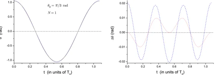
For a not-so-large amplitude such as θ0 = π/3 rad,
the exact solutionθ(t)(black, solid curve), the harmonic approximation (red, dotted curve), our Eq. (17), and the Fourier-based approximation (blue, dashed curve), our Eq. (22), are plotted in Fig. 2. As may be seen, both ap-proximations work well, the harmonic one (relative error <1%) being somewhat better than the Fourier-based approximation taken withjust one term, whose relative error reaches2%. However, the harmonic approximation is much poorer than the Fourier one with N = 2(not included in Fig. 2), whose maximum relative error is only 0.04%.
For θ0=π/2rad, which is the largest amplitude for
smooth oscillations of a pendulum sustained by a flexible
wire, the results are shown in Fig. 3. As seen in the upper panel, the harmonic approximationθ˜(t)seems to remain accurate, but the error graph in the lower panel reveals a maximum relative error of2.3%, much larger than0.2% obtained with N = 2 in the Fourier-based approximation.
For larger amplitudes, a rigid rod is demanded for producing smooth oscillations and the loss of harmonicity is more striking.1 For instance, for θ
0 = 45πrad, the
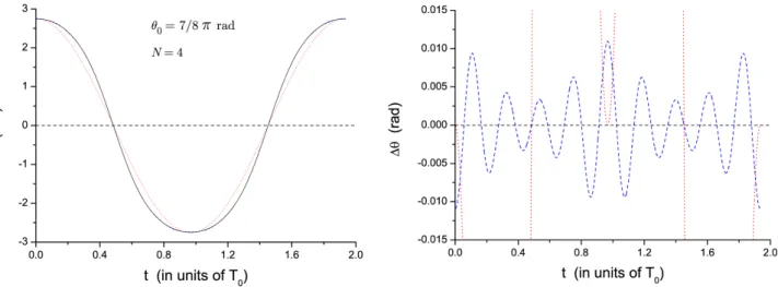
harmonic approximation is highly inaccurate, whereas the Fourier-based approximation withN = 3is accurate to a 0.6% level. Even for amplitudes as large as θ0 =
7
8πrad (i.e., 157.5
◦), as shown in Fig. 4, the Fourier
approximation withN= 4presents a maximum relative 1When the mass of the rod is not negligible in comparison to the
mass of the bob one has aphysical pendulum, for which both the length (i.e., the distance between the center of mass and the suspension point) and the moment of inertia in Eq. (1) must be reconsidered. See Ex. 11.2 of Ref. [12].
Figure 2:Periodic approximations for the exact solutionθ(t)of the pendulum equation, for θ0=π/3rad. Upper panel: the solid
curve (black) is for the exact solution, Eq.(16); the dotted curve (red) is for the harmonic approximationθ˜(t), Eq.(17); and the
dashed curve (blue) is for the Fourier-based approximationθb(t), our Eq.(22), withN = 1only. Note that the solid and dotted
curves are almost indistinguishable, whereas the dashed (blue) curve departs somewhat from that set. Lower panel: deviations from θ(t)withθ˜(t)(dotted curve) andθb(t)(dashed curve).
Figure 4:The same of the previous figures, for θ0= 7
8πrad. The Fourier approximation was taken withN = 4. Again, the solid and dashed curves are practically indistinguishable, whereas the dotted (red) curve departs much from them.
error of only0.4%. Even for very large amplitudes such as θ0= 0.95πrad (i.e.,171◦), the Fourier approximation
withN = 6attains a 0.3%accuracy.
5. Conclusion
In this note, periodic analytical approximations for the exact solution of the pendulum equation of motion are proposed. As a first approximate solution, I have modi-fied theharmonicapproximation proposed in Ref. [17], which resulted in an accurate approximation for ampli-tudes up toπ/3rad. However, due to the unavoidable loss of harmonicity with the increase of amplitude, the harmonic approximation soon becomes poor. In fact, for amplitudes aboveπ/2rad, which are of interest for some experiments [4, 8, 26–28], the deviations are significant, as shown in Fig. 3. Then, I have found it natural to take the periodicity of the exact solution into account to derive an analytical Fourier series expansion, giving continuity to a numerical treatment I have developed (with co-authors) in a very recent work [24]. This task re-vealed many complexities due to the inverse sine function present in the exact solution, our Eq. (16), so I decided to expand only the (periodic) Jacobi elliptic function sn(u;k), rather than the whole functionθ(t). The trunca-tion of this series to only a few terms has revealed itself as a good approximation technique, yielding relative er-rors smaller than 0.4%even for amplitudes as large as
7
8πrad with four terms only, as shown in Fig. 4. A
pre-vious treatment of this sort is not found in the literature and the advantages of the periodic approximate formulae derived here are certainly their simplicity and accuracy, which makes them useful for analysing large-amplitude oscillations in experiments, working well for arbitrarily long time intervals. This kind of periodic approximations may be of general interest for science and engineering applications in which the natural modes of oscillatory structures must be determined accurately, e.g. avoiding
dangerous resonances of buildings in earthquakes [10]. In most real oscillatory systems the inclusion of dissipative effects (e.g., friction and air resistance) is necessary for a more realistic modelling, so the extension of the approach put forward here to dissipative pendular systems is left as a suggestion to the more interested readers.
Acknowledgments
The author wishes to thank M. R. Javier for checking computationally all results in this work.
Supplementary material
The following online material is available for this article: Appendix
References
[1] G. Nicolis,Introduction to nonlinear science(Cambridge University Press, Cambridge, 1995).
[2] P. Amore and A. Aranda, J. Sound Vib. 283, 1115 (2005).
[3] G.L. Baker and J.A. Blackburn,The pendulum: a case study in physics(Oxford, New York, 2005).
[4] W.A. Shelton, K.D. Bonin and T.G. Walker, Phys. Rev. E71, 036204 (2005).
[5] A. Marchenkov, R.W. Simmonds, A. Loshak, J.C. Davis and R.E. Packard, Phys. Rev. B61, 4196 (2000). [6] J.A. Crawford, Text U11610, available in http://
www.am1.us/wp-content/Protected_Papers/ U11610_ Pendulums_and_Elliptic_Integrals_new.pdf
[7] P. Amore, M. Cervantes, A. de Pace and F.M. Fernández, Phys. Rev. D75, 083005 (2007).
[8] G.J. Barclay and I.W. Stewart, J. Phys. A 33, 4599 (2000).
[9] V.E. Grishin and V.K. Fedyanin, Theor. Math. Phys.
[10] A.C. Lazer and P.J. McKenna, SIAM Rev. 32, 537 (1990).
[11] T.H. Fay, Int. J. Math. Educ. Sci. Technol. 34, 527 (2003).
[12] S.T. Thornton and J.B. Marion,Classical Dynamics of Particles and Systems(Brooks/Cole, New York, 2004), 5th ed.
[13] F.M.S. Lima and P. Arun, Am. J. Phys.74, 892 (2006). [14] F.M.S. Lima, Am. J. Phys.78, 1146 (2010).
[15] I.S. Gradshteyn and I.M. Rhyzik, Table of Integrals, Series, and Products(Academic Press, New York, 2007), p. 859, 7th ed.
[16] V. Prasolov and Y. Solovyev, Elliptic functions and integrals(AMS, Providence, 1991), p. 25.
[17] F.M.S. Lima, Eur. J. Phys.29, 1091 (2008).
[18] F.S. Lopes, R.N. Suave and J.A. Nogueira, Rev. Bras. Ens. Fis.40, e3313 (2018).
[19] A. Belendez, E. Arribas, A. Marquez, M. Ortuno and S. Gallego, Eur. J. Phys.32, 1303 (2011).
[20] T.G. Douvropoulos, Eur. J. Phys.33, 207 (2012). [21] N.H. Abel, Journal für die Reine und Angewandte
Math-ematik2, 101 (1827).
[22] C.G.J. Jacobi,Fundamenta nova theoriae functionum ellipticarum(Sumtibus Fratrum, Königsberg, 1829). [23] A.R. Chouikha, J. Nonlinear Math. Phys.12, 162 (2005). [24] I. Singh, P. Arun and F.M.S. Lima, Rev. Bras. Ens. Fis.
40, e1305 (2018).
[25] E.T. Whittaker and G.N. Watson,A Course of Modern Analysis(Cambridge University Press, Cambridge, 1927), 4th ed.
[26] T. Lewowski and K. Wozmiak, Eur. J. Phys. 23, 461 (2002).
[27] S. Gil, A.E. Legarreta and D.E. di Gregorio, Am. J. Phys.
76, 843 (2008).