Asymptotic soliton train solutions of the defocusing nonlinear Schro¨dinger equation
A. M. Kamchatnov,1,2R. A. Kraenkel,2and B. A. Umarov2,3 1
Institute of Spectroscopy, Russian Academy of Sciences, Troitsk 142190, Moscow Region, Russia
2Instituto de Fı´sica Teo´rica, Universidade Estadual Paulista–UNESP, Rua Pamplona 145, 01405-900 Sa˜o Paulo, Brazil 3Physical-Technical Institute, Uzbek Academy of Sciences, 700084 Tashkent-84, G. Mavlyanov Street, 2-b, Uzbekistan
~Received 23 October 2001; revised manuscript received 21 February 2002; published 20 September 2002!
Asymptotic behavior of initially ‘‘large and smooth’’ pulses is investigated at two typical stages of their evolution governed by the defocusing nonlinear Schro¨dinger equation. At first, wave breaking phenomenon is studied in the limit of small dispersion. A solution of the Whitham modulational equations is found for the case of dissipationless shock wave arising after the wave breaking point. Then, asymptotic soliton trains arising eventually from a large and smooth initial pulse are studied by means of a semiclassical method. The parameter varying along the soliton train is calculated from the generalized Bohr-Sommerfeld quantization rule, so that the distribution of eigenvalues depends on two functions—intensityr0(x) of the initial pulse and its initial
chirpv0(x). The influence of the initial chirp on the asymptotic state is investigated. Excellent agreement of
the numerical solution of the defocusing NLS equation with predictions of the asymptotic theory is found.
DOI: 10.1103/PhysRevE.66.036609 PACS number~s!: 42.65.Tg
I. INTRODUCTION
Nonlinear Schro¨dinger ~NLS! equation is a universal equation that describes the evolution of envelopes of linear waves under the influence of weak dispersion and nonlinear effects in a variety of physical systems. Depending on the sign of the nonlinear term in this equation, the focusing and defocusing cases with quite different properties are distin-guished. In particular, the focusing NLS equation has bright soliton solutions propagating on the zero background, whereas defocusing NLS equation does not support bright solitons and instead has dark soliton solutions on the nonzero plane wave oscillating background@1#.
We shall consider here the defocusing NLS equation with initial conditions in the form of a large and smooth pulse described by the intensityr0(x) and chirpv0(x). It is known that in the limit of negligible dispersion a general enough initial dark pulse governed by the defocusing NLS equation evolves at some critical time to the formation of the wave breaking point and taking into account the small dispersion leads to the onset of oscillations just after the wave breaking point @2,3#. The region of oscillations arising here can be presented as a modulated periodic solution of the NLS equa-tion. This permits one to apply to this problem the Whitham theory of modulations@4,5#which was used previously in the solution of similar problems about the evolution of large pulses described by the Korteweg–de Vries ~KdV!equation @6 –9#. Generalization of the Whitham theory on the defocus-ing NLS equation case was developed in Refs.@10–13#. In a general case the solution of the Whitham equations is quite complicated. However, in the vicinity of the wave breaking point the pulse can be described by simplified approximate formulas which admit an exact analytical solution of the Whitham equations in a closed form. For the case of the KdV equation such a solution was found in Refs.@14,15#. Here we shall find a similar solution of Whitham equations for the NLS equation case that describes the so-called dissipation-less shock wave arising after the wave breaking point.
Further evolution of the pulse leads to the stage when
oscillations occupy the whole pulse and they evolve eventu-ally into a train of solitons. As was noticed in Refs.@16,17# for the KdV equation case, the parameters of these asymptotic solitons can be calculated from a semiclassical treatment of the quantum mechanical Schro¨dinger operator associated with the KdV equation in the framework of the inverse scattering transform method with a potential deter-mined by the initial data. Then, for a large pulse leading to a great number of solitons at the final stage, the spectrum can be found with the use of the semiclassical ~Bohr-Sommerfeld!quantization rule that gives a full description of the asymptotic stage of the evolution. The theory developed in Refs. @12# shows that a similar approach applies also to the defocusing NLS equation. Here we shall obtain the nec-essary generalization of the Bohr-Sommerfeld quantization rule by a simple method @18,19#which applies also to many other integrable wave equations. The results obtained permit us to estimate the influence of initial chirp on the evolution of large pulses in optical fibers @2,11,20,21# and other non-linear materials, e.g. magnetic films @22,23#.
II. PERIODIC AND DARK SOLITON SOLUTIONS OF THE DEFOCUSING NLS EQUATION
We shall consider the defocusing NLS equation in the standard dimensionless form
i«ut1«2uxx22uuu2u50, ~1!
where u(x,t) is the envelope amplitude evolving with time t during the propagation of the pulse along x axis and small parameter«!1 controls the relative magnitude of the disper-sion effects. This equation is completely integrable, that is, it can be presented as a compatibility condition of two linear systems @24# cx5Uc, ct5Vc, where U and V are 232
matrices. However, for the investigation of a semiclassical limit it is more convenient to use a scalar representation @19,25#in the form
«2c
xx5Ac, ct5221Bxc1Bcx, ~2!
where
A52
S
l1i« 2ux
u
D
21uuu2
2«
2
2
S
uxxu 2 ux2
u2
D
,B522l1i«ux
u , ~3!
which was first obtained in Ref.@26#. The transition to semi-classical limit is achieved by means of the substitution
u~x,t!5
A
r~x,t!expS
i «E
x
v~x
8
,t!dx8
D
, ~4!so that NLS Eq.~1!transforms into a system of equations for intensityr(x,t) and chirpv(x,t):
1
2rt1~rv!x50, 12vt1v vx1rx1«2~rx2/8r22rxx/4r!x50. ~5!
Thus, in the semiclassical limit «→0 the initial pulse at t
50 is determined by smooth distributions of r0(x) and v0(x), whereas u0(x) may be a fast oscillating function if v0(x)Þ0. We are interested in finding solutions at typical stages of pulse evolution.
As was noticed above, we suppose that arising after the wave breaking point, the regions of oscillations can be pre-sented as modulated periodic waves—soliton trains. Such periodic solutions of Eq.~1!can be obtained as follows. It is easy to check that the functions
c65
A
gexpS
6i«
E
x
A
P~ l !g dx
D
~6!satisfy the first part of Eq.~2!provided that g(x,t) satisfies the equation
«2 ~1
2ggxx2
1 4gx
2
!2Ag25P~ l !, ~7!
where the constant on the right-hand side can only depend on the spectral parameter l. The periodic solution is distin-guished by the condition that P(l) be a polynomial in l, and the one-phase periodic solution corresponds to the fourth degree polynomial
P~ l !5
)
i51 4
~ l2li!5l42s1l31s2l22s3l1s4. ~8!
Then g(x,t) is the first degree polynomial
g~x,t!5m~x,t!2l, ~9!
and by taking l5m in Eq. ~7! we obtain the equation for
m(x,t),
«mx52
A
2P~m!. ~10!From the second part of Eq.~2!we find that g(x,t) satisfies also the equation
gt5Bgx2Bxg, ~11!
which in a similar way yields
mt52s1mx, ~12!
where we have used the identity
m~x,t!5s1/21i«ux/2u ~13!
following from Eq. ~7! after equating coefficients ofl3 on both sides of this formula. Thus,m(x,t) depends only on the phase j5x2s1t and obeys the equation
«dm
dj52
A
2P~m!, j5x2s1t. ~14!The variable m(x,t) is complex and moves along a certain curve in the complex plane determined by the so-called ‘‘re-ality conditions’’~see Ref.@5#!. These conditions distinguish physically meaningful solutions of Eq. ~14!and lead to the following expression for the intensity of the nonlinear peri-odic wave:
r~x,t!5uu~x,t!u2
5 14~ l12l22l31l4!2
1~ l12l2!~ l32l4!
3sn2@
A
~ l12l3!~ l22l4!j/«,m#, ~15! where the zeros li,i51,2,3,4, are ordered according tol1>l2>l3>l4, ~16!
the parameter m of the elliptic function is defined by
m5~ l12l2!~ l32l4! ~ l12l3!~ l22l4!
, ~17!
and
j5x2Vt, V5s15
(
i51 4
li, ~18!
V being the phase velocity of the nonlinear wave.
In a weakly modulated nonlinear periodic wave the pa-rameters li,i51,2,3,4, become slow functions of x and t
which change little in one wavelength and one period. The evolution of li is governed by the Whitham modulation equations ~obtained for the NLS equation case in Refs. @27,28#!
]li
]t 1vi~ l !
]li
]x 50, i51,2,3,4, ~19!
where the Whitham velocities are equal to
vi~ l !5
S
12 L]iL
]i
D
V, ]i[]/]li, i51,2,3,4,and L(l) is a wavelength
L5 K~m!
A
~ l12l4!~ l22l3!, ~21!
K(m) being the complete elliptic integral of the first kind. Substitution of Eq. ~21! into Eq. ~20! gives the Whitham velocities in the form
v15
(
li12~ l12l2!~ l12l4!K ~ l12l4!K2~ l22l4!E
,
v25
(
li22~ l12l2!~ l22l4!K ~ l22l3!K2~ l12l3!E
, ~22!
v35
(
li12~ l22l3!~ l32l4!K ~ l22l3!K2~ l22l4!E
,
v45
(
li22~ l12l3!~ l32l4!K ~ l12l4!K2~ l12l3!E
,
where K5K(m) and E5E(m) are complete elliptic inte-grals of the first and second kind, respectively. In this case the parameters li are called Riemann invariants of the
Whitham equations and our first task is to find their solution corresponding to the region of oscillations arising after the wave breaking point. At one edge of this region we have m
51 orl35l2, so that the intensity distribution is given by
rs~x,t!5
1
4~ l12l4! 2
2 ~ l12l2!~ l22l4!
cosh2@
A
~ l12l2!~ l22l4!j/«# , ~23!where j5x2(l112l21l4)t, and at the other side with m50 wherel25l1 we obtain a smooth solution
r~x,t!514~ l32l4!2. ~24!
Thus, in the problem of the evolution of dissipationless shock wave we have to find boundaries of the region of oscillations and the dependence of the parameters li on x
and t within it.
At the asymptotically large values of time the pulse evolves into a train of dark soliton solutions with m51 @Eq. ~23!#. The values ofl1 andl4 are determined by the back-ground wave and hence are constant, so that the parameters of solitons in the train are determined by the values of l2. Our second task is to find how l2 varies along the soliton train arising from the initial pulse with given distributions of
r0(x) andv0(x).
III. DISSIPATIONLESS SHOCK WAVE
For smooth pulses, when we can neglect higher space derivatives in Eqs. ~5!, we arrive at equations of hydrody-namical type,
1
2rt1~rv!x50,
1
2vt1v vx1rx50, ~25!
which correspond to the dispersionless limit of the NLS equation ~1!. It is convenient to introduce variables called Riemann invariants,
l651
2v6
A
r, ~26!so that Eqs.~25!take a convenient symmetric form
]l1
]t 1~3l11l2!
]l1
]x 50,
]l2
]t 1~ l113l2!
]l2
]x 50. ~27!
Initial data are given by two functionsl1(x,0) andl2(x,0) determined by the initial distributions r0(x) andv0(x). The system~27!leads to two families of characteristics, i.e. lines in the (x,t) plane along which one of the two Riemann in-variants ~either l1 or l2) is constant. The wave breaking point corresponds to the moment when characteristics of one of the families begin to intersect each other, so that the cor-responding Riemann invariant becomes a three-valued func-tion of the space coordinate. Let such an intersecfunc-tion occur for the characteristics with constant l1. Then at the wave breaking point the profile of l1 as a function of x has a vertical tangent line and, hence, in the vicinity of this point it varies very fast, whereas the second Riemann invariant var-ies with x much slower and may be considered here as a constant parameter,
l25l05const. ~28!
Thus, the second part of Eq.~27! is solved by Eq.~28!and the first part of Eq.~27!has a well-known solution
x2~3l11l0!t5f~ l1!.
Since at the wave breaking time moment t50 the function x5f (l1) must have an inflection point with a vertical tan-gent line, in the vicinity of this point f (l1) can be approxi-mated by a cubic function,
x2~3l11l0!t52C~ l12l¯1!
3. ~29!
Equations~28!and~29! ~at t50) may be considered as ini-tial data for the Riemann invariants in the vicinity of the wave breaking point.
The ‘‘shallow water equations’’ ~25! are invariant with respect to the Galileo transformation,
x
8
5x22v0t, t8
5t, r5r8
, v5v8
1v0,l65l6
8
11 2v0, and scaling transformationx5ax
8
, t5t8
, r5a2r8
, v5av8
, l65al6
8
,which allow us to transform Eqs. ~28!and~29! to a simple form
x2~3l11¯l!t52l
1
3 , l
where we use the previous notation~without primes!for the Riemann invariants and space and time coordinates. Thus, in the dispersionless limit the solution of Eqs.~27!has the form ~30!in the vicinity of the wave breaking point~see Fig. 1!.
The formation of a multivalued region of l1(x) shows that we cannot neglect dispersion in the vicinity of this point. The dispersion effects lead to the formation of the region of oscillations where the solution of the NLS equation ~1! can be approximated by a modulated periodic wave. In our ap-proximation we suppose thatl4 is constant within the region of oscillations and l1, l2, andl3 vary so that at one of its boundaries we havel25l3 (m51) and at the other bound-ary l25l1 (m50). Correspondingly, the Whitham veloci-ties~22!are equal at these limits to
v153l11l4, v25v35
(
li, v45l113l4 ~31!atl25l3(m51), and to
v15v25
(
li14~ l12l3!~ l12l4!
2l12l32l4 , v353l31l4,
v45l313l4 ~32!
at l25l1(m50). Hence, two of the four Whitham equa-tions~19!reduce to Eqs.~27!at the boundaries of the region of oscillations, and therefore the corresponding Riemann in-variants have to coincide withl6 at these boundaries,
l15l1 at m51, l35l1 at m50,
and l45l2 in both cases. ~33!
Thus we have to find such a solution of Eqs. ~19! which gives
x2~3l11l4!t52l13 at m
51, ~34!
x2~3l31l4!t52l33 at m
50.
In the generalized hodograph method@29#the solution is looked for in the form
x2vi~ l !t5wi~ l !, i51,2,3,4, ~35!
wherevi(l) are the Whitham velocities ~20!and wi(l) are velocities of a flow
]li
]t 1wi~ l !
]li
]x 50, i51,2,3,4, ~36!
commuting with Eqs.~19!. If we represent wi(l) in the form
analogous to Eqs. ~20!,
wi~ l !5
S
12 L]iL
]i
D
W, i51,2,3,4, ~37!then the condition of commutativity of flows ~19!and ~36! reduces to the Euler-Poisson equations@10#
]i]jW2
1 2~ li2lj!
~]iW2]jW!50, iÞj. ~38!
It is easy to check that this equation has a particular solution W5const/
A
P(l), P(l)5)(l2li), which is sufficient forour aim. We choose the normalization factor so that the co-efficient before l21 in the series expansion of W in powers of l21 be equal to s
1 and, hence, the corresponding wi
co-incide with the Whitham velocities ~20!. Thus, we obtain a sequence of W5W(k) defined by the generating function
W5 2l 2
A
P~ l !5(
W(k)lk 521 s1
l 1
3 8s1
2
221s2
l2
~39!
1 5 16s1
3
234s1s2112s3
l3 1• • •,
where P(l) coincides with the polynomial in Eq.~8!. Thus, a sequence of velocities of the commuting flows is given by
wi(k)5W(k)1~vi2s1!]iW(k). ~40!
Then a simple calculation shows that the solution~35! satis-fying the boundary conditions~34!has the form
x2vi~ l !t52 8
35wi
(3)
~ l !1354 l¯ wi
(2)
1351 l¯
2v
i~ l !1
1 35¯l
3,
i51,2,3; ~41!
l45¯l5const.
These formulas give the solution of our problem in an im-plicit form.
Let us find the laws of motion of the boundaries of the oscillatory region. At m51 Eqs. ~41! with i51 and i53 give
x2~3l11l¯!t52l1 3 ,
x2~ l112l31l¯!t52
1 35~5l1
3
16l12l318l1l3 2
116l33!,
and their difference gives the relation
t5351 ~15l1 2
112l1l318l3 2
!. ~42!
The other two equations of Eq.~41!expanded into series in powers of l2
8
5l22l3 yield after subtraction another rela-tiont5351 ~3l1 2
18l1l3124l3
2!. ~43!
Equating~42!and~43!to each other, we find at this bound-ary the relation
l352
3
4l1, ~44!
which coincides with an analogous relation in the KdV equa-tion case@5,14#. Then from Eqs.~42!or~43!we obtain at the left boundary t5103l1
2
and hence the left boundary of the region of oscillations moves according to the law
x2~t!5~3l
11¯l!t2l1 3
5¯ tl 213
A
10 3t
3/2. ~45!
Analogous calculation at m50 (l25l1) yields the relations
t5~8l127l ¯!~8l
1 2
14l1l313l32
!215l33 35~4l12l323l¯!
, ~46!
21l¯2
~4l11l3!210l¯~20l1 2
12l1l31l3 2
!116l1~8l12
2l1l32l3 2!
19l33
50. ~47!
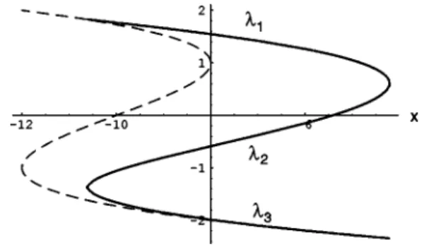
In the limit ul¯u→`, these equation reproduce the relations for the KdV equation case@5,14#, in particular,l15214l3. However, in the NLS equation case the solution ~41!is not self-similar and depends on the parameter¯ . An example ofl the dependence of the Riemann invariantsl1,l2,l3on x at a fixed value of t is shown in Fig. 2. Substitution of these functionsli(x) into Eq.~15!gives the dependence of
inten-sity on x shown in Fig. 3. This plot illustrates the process of the formation of a shock for the NLS equation case.
IV. ASYMPTOTIC STAGE OF EVOLUTION
In the asymptotic stage of the evolution the pulse decays into a set of solitons which can be presented as modulated one-phase periodic soliton trains. Each separate soliton is described by Eq.~23!and parametersl1andl4are constant along the train, whereas the parameterl2 changes its value from one soliton to another. Thus, the properties of the train
are determined by the spectrum of values l2. It is known that this spectrum coincides with the eigenvalues of the first part of Eq. ~2! for given r0(x) and v0(x) and it does not change during the evolution of u(x,t) governed by the NLS equation. In the case of large and smooth pulses with large number of eigenvalues, the spectrum can be determined, in principle, by means of a semiclassical treatment of the eigen-value problem. The corresponding generalization of semi-classical quantization rules can be found with the use of a matrix ~Zakharov-Shabat! spectral problem associated with the NLS equation~see, e.g., Refs.@12,30–32#!. Here we shall show that it follows very simply from the scalar form ~2!, and this method of derivation can be generalized on many other integrable equations~see Refs. @19,25#!.
For strictly periodic case, the solution of the second-order Eq.~2!is given by Eq.~6!with constant P(l). For a slowly modulated wave the zeroslibecome slow functions of x and t, and for this reason we inserted P(l) under the integration sign in Eq.~6!. With the use of Eqs.~7!,~9!, and~13!, we can present c6 in the form
c6;exp
S
6i«
E
x1
g$@~ l1i«ux/2u! 2
2uuu2
1«2
~uxx/2u2ux
2/2u2
!#g21«2
~ggxx/22gx
2
/4!%1/2dx
D
,~48!
FIG. 2. The dependence of Riemann invariantsl1,l2,l3on x
at fixed value of time t51. The fourth Riemann invariantl45l¯
5210 is not depicted. The dashed line shows the corresponding dependence ofl1for the solution of equations in the dispersionless limit.
FIG. 3. Dissipationless shock wave for the NLS equation case. The plot corresponds to the time t51 and l45l¯5210, and «
where
g5s1/21i«ux/2u2l. ~49!
We suppose that this expression holds approximately for all moments of time including the initial state. Then, since the initial distributions of r0(x)5uu(x,0)u2 and v0(x)5
2i«ux/u are supposed to be smooth functions of x, we can
neglect the derivatives ofv0(x) in the weak dispersion limit «2
!1 to obtain the WKB wave function of the initial state,
cWKB;exp
S
6 i «E
x
A
@l212v0~x!#22r0~x!dx
D
. ~50!The eigenvalues l are determined in this approximation by the well-known Bohr-Sommerfeld quantization rule@33#
1
«
R
p~x!dx52p~n11
2!, n50,1,2, . . . ,N,
p~x!5
A
@l212v0~x!#22r0~x!, ~51!
where the integration is taken over the cycle around two turning points where the integrand function vanishes. Eigen-values found in this way are equal to the Eigen-values of the pa-rameter l2 in soliton solution ~23! when solitons are well separated from each other in the asymptotic soliton train.
It is instructive to note that the rule ~51! corresponds to the semiclassical quantization of a mechanical system with the Hamiltonian
H~p,x!5@
A
p21r0~x!21
2v0~x!#2, ~52! where x is a coordinate and p a momentum. At the turning points the momentum p vanishes. Equation ~51! states that the area inside the contour H( p,x)5const in the phase plane (x, p) can only take half-integer values in units of 2p«.
The regions of the possible values ofl are determined by the condition that the expression under the square root in Eq. ~51! is positive and has two real turning points. Thus the plots of the ‘‘potentials’’ ~Riemann invariants in the zero dispersion limit!
l6~x!51
2v0~x!6
A
r0~x! ~53!permit one to find a qualitative picture of the spectrum. In particular, if the chirp vanishes at infinity, v0(x)→0 at uxu
→`, the greatest absolute value of l2 is approximately equal to
ul2umax5
A
r~ ` !512~ l12l4!. ~54!On the other hand, the smallest absolute values of ul2u for large initial pulse must be very close to the absolute local minima of the potentialsul6(x)u and at the same time coin-cide with the amplitudes of the deepest solitons
A
rs@see Eq.~23!# in the trains produced by this pulse. This gives the relation
1
4~ l12l4!
2
2~ l12l2!~ l22l4!5l2 2,
which is satisfied by
l25
1
4~ l11l4! or l11l450.
Here the first solution is nonphysical because for symmetri-cal pulses we always have l452l1 but ul2umin must vary
depending on the initial data. Thus, we conclude that in the asymptotic trains of solitons the constant parameters satisfy the relation
l452l1, ~55!
and hence the possible values of l2 are located inside the intervals
2lmax,l2,lmin
8
, lmin9
,l2,lmax, ~56!wherelmax5
A
r(`) andl8
,l9
(l8
,l9
) correspond to theminima of the potentials ul6(x)u. Solitons in the arising
trains have the intensity given by
rs~x,t!5l1 2
2
l12
2l22
cosh2@
A
l122l22
~x22l2t!/«#
. ~57!
Since the velocity of solitons ~57! is equal to the values of 2l2 and at this asymptotic stage of the evolution we can neglect the ‘‘initial positions’’ of solitons, then the coordinate of the nth soliton at the moment t is given by
x52l2(n)t, ~58!
where l2(n) is the nth eigenvalue determined by Eq. ~51!. Hence, at the moment t the soliton trains occupy the intervals
22lmaxt,x,2lmin
8
t and 2lmin9
t,x,2lmaxt.~59!
Differentiation of Eq. ~51! with respect to l yields the number of eigenvalues in the interval (l,l1dl),
dn5f~ l !dl5
S
1 2p«R
l2v0~x!/2
A
@l2v0~x!/2#22r0~x!dx
D
dl. ~60!This formula has a simple interpretation in terms of semi-classical quantization rules for the Hamiltonian ~52!. Namely, the ‘‘velocity of motion’’ between two turning points is given by
x˙5]H
]p5
2l
A
~ l2v0~x!/2!22r0~x! l2v0~x!/2 ,and the calculation of the period of this oscillatory motion T5rdx/x˙ and of the corresponding frequency v52p/T shows that Eq. ~60!can be written in the form
dl2
dn 5«v~ l !52p«
S
R
dxx˙
D
21
which means that the distance between neighboring eigen-values of l2 is equal to the ‘‘quantum’’«v proportional to the frequencyv of the classical motion. The rule~61! coin-cides with the quantum mechanical rule of semiclassical quantization with the Planck constant \ replaced by« @33#. The number of solitons in the interval (x,x1dx) is given by
dn5~1/2t!f~x/2t!dx, ~62!
where f (l) is determined by Eq. ~60!. The amplitudes of these dark solitons are equal to l12
2(l2(n))2, and positive eigenvalues l2(n).0 correspond to solitons moving to the right and negative eigenvaluesl2(n),0 to solitons moving to the left. Thus, the formulas obtained give the complete de-scriptions of the soliton trains arising from an initially large and smooth pulse.
Let us illustrate this theory by concrete examples and compare the theoretical predictions with the results of the direct numerical solution of the defocusing NLS equation ~1!.
At first we choose the initial distribution of intensity
r0(x) in the form
r0~x!5
S
22 1 cosh xD
2
~63!
and the initial distribution of v0(x) as
either v0~x!50 ~64a! or
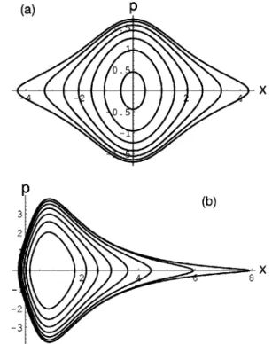
v0~x!524sinh x/cosh2x. ~64b! The parameter « controlling the dispersion effects is chosen equal to «50.2. In Fig. 4 the plots of potentials ~53! are shown for zero ~a!and nonzero ~b!initial velocities v0(x). The possible values ofl are located inside the intervals~56! and they must satisfy the quantization rule ~51! that selects contours H( p,x)5const5l2 in the phase plane (x, p). These contours corresponding to the even values of n and l.0 are depicted in Fig. 5 for zero ~a! and nonzero ~b! initial chirp. The dependence of n on l.0 is shown in Fig. 6, where the lower curve corresponds to zero chirp and the
FIG. 4. Plots of initial potentialsl6@see Eq.~53!#as functions of x forr0(x) andv0(x) given by Eqs.~63!and~64!,~a!and~b!,
respectively. The turning points x6corresponding to the eigenvalue
l51.2 are shown. The possible values ofl are given by Eq.~65!.
FIG. 5. Contours H( p,x)5const5l2in the phase plane (x, p)
of the mechanical system described by Hamiltonian~52!withr0(x)
and v0(x) given by Eqs. ~63! and ~64a,b! and for values of l
determined by the quantization rule~51!with even n.
FIG. 6. The dependence of n on l.0 defined by Eq.~51!for
r0(x) and v0(x) given by Eqs. ~63! and ~64!. The lower curve
corresponds to zero chirp~a!and the upper curve to nonzero chirp
upper curve to nonzero chirp. As we see, the chosen chirp diminishes the values of the eigenvalues l2(n), so that soli-tons arising in this case move slower than in the case of zero chirp.
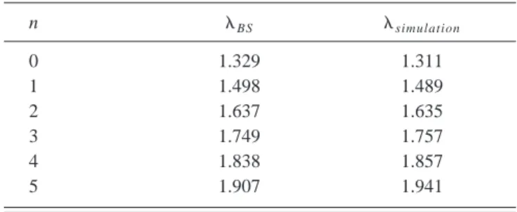
We have solved the NLS equation~1!with the initial con-ditions~63! and~64!numerically and the results are shown in Fig. 7 again for zero~a!and nonzero~b!chirp. As one can see, the results are in excellent agreement with the predicted intervals. To make a comparison of the theory with numeri-cal results clearer, we have numeri-calculated velocities of solitons in the trains and, according to Eq.~58!, have taken halves of
these velocities as values of l2 calculated numerically. We give in Table I the values of l2[lBS calculated from the Bohr-Sommerfeld quantization rule ~51! and of l2 [lsimulation calculated from velocities of the soliton trains.
The agreement between the two methods of calculation is quite good. The difference does not exceed 3% and is maxi-mal at very smaxi-mall n, where the accuracy of the semiclassical calculation of the eigenvalues cannot, generally speaking, be extremely high, and at large n, where the numerical estimate has poor accuracy because solitons here are not separated well enough from each other and their motion does not obey the formula ~58! yet. The accuracy of asymptotic formulas increases with the decrease of «. The number of solitons formed from a pulse with a given intensity is proportional to«.
FIG. 7. Soliton trains obtained by numerical solution of the NLS equation ~1!with«50.2 and initial conditions~63! and~64! with zero ~a! and nonzero ~b! initial chirp. Asymptotic distributions of intensity are shown as functions of space coordinate x at the mo-ment t525.
FIG. 8. The potentialsl6(x) @see Eq.~53!#for the initial con-ditions~63!and~65!.
FIG. 9. Soliton trains obtained by numerical solution of the NLS equation ~1! with«50.2 and initial conditions~63! and~65!. The asymptotic distribution of intensity is shown as a function of space coordinate x at the moment t520. The train of usual solitons moves to the left and corresponds to negative eigenvalues in the potential
l2(x) and the train of twin solitons moves to the right and corre-sponds to positive slightly split eigenvalues in two-well potential
l1(x).
TABLE I. Eigenvalues for the initial conditions~63!and~64!.
n v50
v52
4sinh x cosh2x
lBS lsimulation lBS lsimulation
As a second example we shall consider the initial pulse with intensity~63!and more complicated chirp
v0~x!5 d
dx
S
2sinh x cosh2xD
532cosh~2x!
cosh3x ~65!
when the potentials~53!have the form shown in Fig. 8. The potentiall2(x) has usual one-well form with nondegenerate negative eigenvalues which can be calculated according to the semiclassical rule~51!. However, the semiclassical eigen-values of the two-well potentiall1(x) are double degenerate and by analogy with quantum mechanics they must be split into two very close levels with splitting proportional to the barrier penetration coefficient @33#,
Dl2(n)}exp
S
21«
E
2x1 x1
U
p~x!U
dxD
, ~66!so that the eigenvalues are given by l2(n)65l
2 (n)
612Dl2 (n)
, ~67!
wherel2(n)correspond to the rule~51!and the integral in Eq. ~66! is calculated atl5l2(n). These close to each other ei-genvalues must lead to the formation of ‘‘twin’’ solitons with very close values of their parameters. The intensity of the pulse obtained by the numerical solution of the NLS equa-tion ~1! with initial data ~63! and ~65! is shown in Fig. 9. Solitons moving to the left correspond to the nondegenerate eigenvalues and their velocities 2l2(n) agree quite well with ones calculated according to Eq. ~51!; see Table II. Twin
solitons moving to the right correspond to slightly split ei-genvalues of the spectral problem with two-well potential l1(x) and the mean velocity of each couple agrees well
enough with the semiclassical rule ~51!; see Table III.
V. CONCLUSION
The semiclassical approach developed in this paper per-mitted us to consider in some detail the evolution of pulses governed by the defocusing NLS equation. Two characteris-tic stages of evolution have been considered—the formation of the dissipationless shock after the wave breaking point and asymptotic soliton trains formed eventually from a large initial pulse. It has been shown that the semiclassical ap-proach to the calculation of the eigenvalues of the problem ~2! yields a simple and effective description of the asymptotic stage of the evolution of an initially large and smooth pulse in the weak dispersion limit. The results show that the arising solitons can be slowed down by the initial chirp, but it cannot prevent the formation of solitons from a large pulse due to dispersion effects. As typical examples, the usual soliton trains and twin soliton trains are considered. Their characteristic features are controlled by the initial con-ditions, what may occur useful for applications. The theoret-ical predictions are confirmed by numertheoret-ical simulations.
ACKNOWLEDGMENTS
A.M.K. and B.A.U. are grateful to the staff of Instituto de Fı´sica Teo´rica, UNESP ~where this work was started! for kind hospitality. The authors were partially supported by FAPESP~Brazil!. A.M.K. thanks also RFBR~Grant No. 01-01-00696!, R.A.K. thanks CNPq~Brazil!, and B.A.U. thanks CRDF ~Grant No. ZM2–2095!for partial support.
@1#Yu.S. Kivshar and B. Luther-Davies, Phys. Rep. 298, 81
~1998!.
@2#M.G. Forest and K.T.-R. McLaughlin, J. Nonlinear Sci. 7, 43
~1998!.
@3#O.C. Wright, M.G. Forest and K.T.-R. McLaughlin, Phys. Lett. A 257, 170~1999!.
@4#G.B. Whitham, Linear and Nonlinear Waves ~ Wiley-Interscience, New York, 1974!.
@5#A.M. Kamchatnov, Nonlinear Periodic Waves and Their
Modulations—An Introductory Course~World Scientific, Sin-gapore, 2000!.
@6#A.V. Gurevich and L.P. Pitaevskii, Zh. E´ ksp. Teor Fiz. 65, 590
~1973! @Sov. Phys. JETP 38, 291~1973!#.
@7#P.D. Lax and C.D. Levermore, Commun. Pure Appl. Math. 36, 253~1983!; 36, 571~1983!; 36, 809~1983!.
@8#A.V. Gurevich, A.L. Krylov and G.A. El, Zh. E´ ksp. Teor. Fiz TABLE II. Negative eigenvalues for the initial conditions~63!
and~65!.
n lBS lsimulation
0 20.2278 20.2280
1 20.6073 20.6052
2 20.9175 20.9155
3 21.1775 21.1774
4 21.39684 21.3998
5 21.58083 21.5875
6 21.73217 21.7432
7 21.85163 21.8695
8 21.93821 21.9647
9 21.98889
TABLE III. Positive eigenvalues for the initial conditions~63!
and ~65!;lsimulation are calculated as arithmetic mean values for
each couple of twin solitons.
n lBS lsimulation
0 1.329 1.311
1 1.498 1.489
2 1.637 1.635
3 1.749 1.757
4 1.838 1.857
101 1797~1992! @Sov. Phys. JETP 74, 957~1992!#.
@9#F.R. Tian, Commun. Pure Appl. Math. 46, 1093~1993!.
@10#G.A. El and A.L. Krylov, Phys. Lett. A 203, 77~1995!.
@11#Y. Kodama, SIAM~Soc. Ind. Appl. Math.!J. Appl. Math. 59, 2162~1999!.
@12#S. Jin, C.D. Levermore, and D.W. McLaughlin, Commun. Pure Appl. Math. 52, 613~1999!.
@13#F.-R. Tian and J. Ye, Commun. Pure Appl. Math. 52, 655
~1999!.
@14#G.V. Potemin, Usp. Matem. Nauk, 43 211~1988! @Russ. Math. Surveys 43, 252~1988!#.
@15#O.C. Wright, Commun. Pure Appl. Math. 46, 423~1993!.
@16#V.I. Karpman, Phys. Lett. A25, 708~1967!.
@17#V.I. Karpman, Nonlinear Waves in Dispersive Media ~ Perga-mon, Oxford, 1975!.
@18#M.S. Alber, G.G. Luther, and J.E. Marsden, Nonlinearity 10, 223~1997!.
@19#A.M. Kamchatnov, R.A. Kraenkel, and B.A. Umarov, Phys. Lett. A 287, 223~2001!.
@20#Y. Kodama and S. Wabnitz, Opt. Lett. 20, 2291~1995!.
@21#D. Kro¨kel, N.J. Halas, G. Giuliani, and D. Grischkowsky, Phys. Rev. Lett. 60, 29~1988!.
@22#M. Chen, M.A. Tsankov, J.M. Nash, and C.E. Patton, Phys. Rev. Lett. 70, 1707~1993!.
@23#A.N. Slavin, Yu.S. Kivshar, E.A. Ostrovskaya and H. Benner, Phys. Rev. Lett. 82, 2583~1999!.
@24#V.E. Zakharov and A.B. Shabat, Zh. Eks. Teor. Fiz. 64 1627
~1972! @Sov. Phys. JETP 37, 823~1973!#.
@25#A.M. Kamchatnov and R.A. Kraenkel, J. Phys. A 35, L13
~2002!.
@26#S.J. Alber, in Nonlinear Processes in Physics, edited by A.S. Fokas et al.~Springer, Berlin, 1993!, p. 6.
@27#M.G. Forest and J.E. Lee, in Oscillation Theory, Computation,
and Methods of Compensated Compactness, edited by C.
Da-fermos, J.L. Erickson, D. Kinderleher, and M. Slemrod, IMA Volumes on Mathematics and its Applications 2 ~Springer, New York, 1986!.
@28#M.V. Pavlov, Teor. Mat. Fiz. 71, 351 ~1987! @Theor. Math. Phys. 71 584~1987!#.
@29#S.P. Tsarev, Izv. Akad. Nauk SSSR Ser. Matem. 54, 1048
~1990! @Math. USSR Izv. 37, 397~1991!#.
@30#J.C. Bronski, Physica D 97, 376~1996!.
@31#P.D. Miller, Physica D 152-153, 145~2001!.
@32#J.C. Bronski, Physica D 152-153, 163~2001!.