Calibration methods for the Hargreaves-Samani equation

2018 | Lavras | Editora UFLA | www.editora.ufla.br | www.scielo.br/cagro

http://dx.doi.org/10.1590/1413-70542018421017517

Calibration methods for the Hargreaves-Samani equation

Métodos de calibração para a equação de Hargreaves-Samani

Lucas Borges Ferreira1*_{, Fernando França da Cunha}1_{, Anunciene Barbosa Duarte}2_, Gilberto Chohaku Sediyama1_{, Paulo Roberto Cecon}3

1_{Universidade Federal de Viçosa/UFV, Departamento de Engenharia Agrícola, Viçosa, MG, Brasil} 2_{Universidade Federal de Viçosa/UFV, Departamento de Fitotecnia, Viçosa, MG, Brasil} 3_{Universidade Federal de Viçosa/UFV, Departamento de Estatística, Viçosa, MG, Brasil} *_{Corresponding author: contato.lucasbf@gmail.com}

Received in June 22, 2017 and approved in September 6, 2017

ABSTRACT

The estimation of the reference evapotranspiration is an important factor for hydrological studies, design and management of irrigation systems, among others. The Penman Monteith equation presents high precision and accuracy in the estimation of this variable. However, its use becomes limited due to the large number of required meteorological data. In this context, the Hargreaves-Samani equation could be used as alternative, although, for a better performance a local calibration is required. Thus, the aim was to compare the calibration process of the Hargreaves-Samani equation by linear regression, by adjustment of the coefficients (A and B) and exponent (C) of the equation and by combinations of the two previous alternatives. Daily data from 6 weather stations, located in the state of Minas Gerais, from the period 1997 to 2016 were used. The calibration of the Hargreaves-Samani equation was performed in five ways: calibration by linear regression, adjustment of parameter “A”, adjustment of parameters “A” and “C”, adjustment of parameters “A”, “B” and “C” and adjustment of parameters “A”, “B” and “C” followed by calibration by linear regression. The performances of the models were evaluated based on the statistical indicators mean absolute error, mean bias error, Willmott’s index of agreement, correlation coefficient and performance index. All the studied methodologies promoted better estimations of reference evapotranspiration. The simultaneous adjustment of the empirical parameters “A”, “B” and “C” was the best alternative for calibration of the Hargreaves-Samani equation.

Index terms: Evapotranspiration; irrigation; temperature; agrometeorology.

RESUMO

A estimativa da evapotranspiração de referência é um importante fator para estudos hidrológicos, projeto e manejo de sistemas de irrigação, dentre outros. A equação de Penman Monteith apresenta elevada precisão e acurácia na estimativa desta variável. No entanto, o uso desta se torna limitado devido ao grande número de dados meteorológicos requeridos. Neste contexto, a equação de Hargreaves-Samani pode ser utilizada como alternativa, contudo, requer uma calibração local para a obtenção de melhores performances. Assim, objetivou-se comparar o processo de calibração da equação de Hargreaves-Samani via regressão linear, via ajuste dos coeficientes (A e B) e expoente (C) da equação e via combinações das duas alternativas anteriores. Foram utilizados dados diários de 6 estações meteorológicas, situadas no estado de Minas Gerais, do período de 1997 a 2016. A calibração da equação de Hargreaves-Samani foi realizada de cinco formas: calibração via regressão linear, ajuste do parâmetro “A”, ajuste dos parâmetros “A” e “C”, ajuste dos parâmetros “A”, “B” e “C” e ajuste dos parâmetros “A”, “B” e “C” seguido de calibração por regressão linear. As performances dos modelos foram avaliadas com base nos indicadores estatísticos erro absoluto médio, erro de viés médio, índice de concordância de Willmott, coeficiente de correlação e índice de desempenho. Todas as metodologias estudadas promoveram melhores estimativas da evapotranspiração de referência. O ajuste simultâneo dos parâmetros empíricos “A”, “B” e “C” foi a melhor alternativa para calibração da equação de Hargreaves-Samani.

Termos para indexação: Evapotranspiração; irrigação; temperatura; agrometeorologia.

INTRODUCTION

The estimation of the reference evapotranspiration (ET_o) is an important factor for hydrological studies, design and management of irrigation systems, agricultural planning, among others. Although exists several equations for ET_o estimation, the Penman-Monteith equation (PM) was proposed by the Food and Agriculture Organization (FAO) as the standard method to be used in any region of the world (Allen et al., 1998).

In places with low availability of meteorological data it is possible to use alternative equations, which require a smaller number of input parameters. In this context, Allen et al. (1998) recommend the use of the Hargreaves-Samani (HS) equation, proposed by Hargreaves and Samani (1985), when only air temperature data is available.

The HS equation is recognized for presenting reasonable performance in several parts of the world (Allen et al., 1998; Almorox; Quej; Martí, 2015). However, as it is an empirical equation, it presents performance varying according to the climatic characteristics of the region where it is used (Sentelhas; Gillespie; Santos, 2010; Maestre-Valero; Martínez-Álvarez; González-Real, 2013). Thus, to better estimate ET_o, the local calibration is recommended (Borges Júnior et al., 2012; Feng et al., 2017). In Brazil, several authors calibrated HS equation for different locations (Arraes et al., 2016; Lima Junior et al., 2016; Borges Júnior et al., 2017).

Many studies were developed aiming the calibration of the HS equation. Among the main techniques used for this purpose, the most commons are the calibration using simple linear regression (Allen et al., 1998; Cobaner, 2011)

and the adjustment of the coefficients and exponent of the

equation (Fernandes et al., 2012; Bogawski; Bednorz, 2014; Martí et al., 2015).

Despite the existence of several studies dealing with calibration of equations for ET_o estimation, there is

still a gap about the efficiency of the calibration methods

used. This is due to the fact that, in most cases, the authors use only one or at most two calibration methods in the

same study, making it difficult to establish comparisons

between them.

The use of more appropriate calibration techniques can lead to better results. In this sense, this study had the objective to compare the calibration process of the HS equation by linear regression, by adjustment of the coefficients and exponent of the equation and by combinations of the two previous alternatives.

MATERIAL AND METHODS

For the development of the study daily data from 6 weather stations of the period 1997 to 2016 were used. The data were obtained from the Banco de Dados Meteorológicos para Ensino e Pesquisa (BDMEP), a meteorological database of the National Institute of Meteorology (INMET) of Brazil. The selected weather stations are located in the municipalities of Januária, Lavras, Paracatu, Sete Lagoas, Uberaba and Viçosa, all in the state of Minas Gerais, Brazil (Figure 1). The geographic coordinates and altitude of each

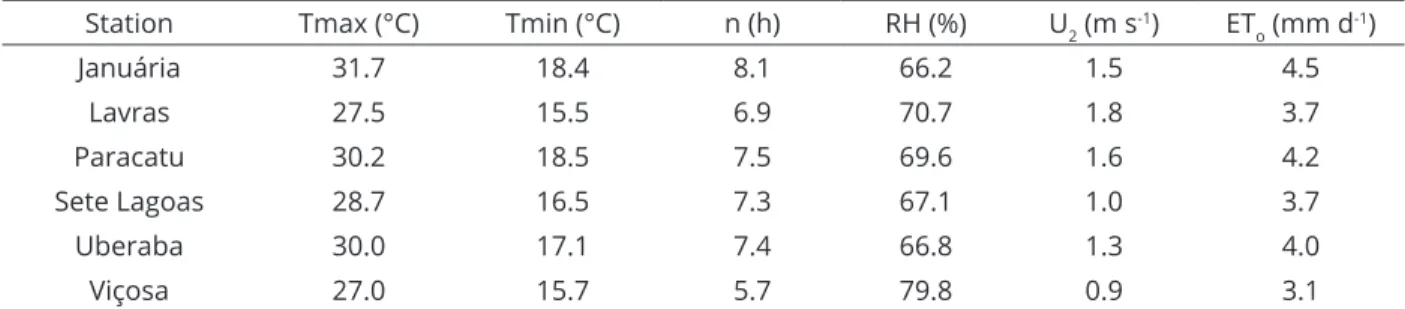
station, as well as the mean values of the weather elements are shown in Tables 1 and 2, respectively.

The used data include maximum and minimum air temperatures (°C), relative humidity (%), sunshine duration (h) and wind speed (m s-1_{). The wind speed,} measured at 10 m height, was subsequently converted to 2 m, as recommended by Allen et al. (1998). Was also performed, with the aid of an algorithm written in the Java programming language, a preprocessing of the data, eliminating days with missing or inconsistent data. Inconsistent data in this work were: minimum temperature greater than the maximum temperature, negative sunshine duration or greater than the maximum possible sunshine duration, negative relative humidity or greater than 100% and negative wind speed (10 m height) or greater than 20 m s-1_{. Given the data conditions, none} additional approach was necessary to overcome quality problems.

For calibration of the Hargreaves-Samani (HS) equation, the daily reference evapotranspiration (ET_o) obtained by the Penman-Monteith (PM) method (Allen et al., 1998) was adopted as standard and calculated according to Equation 1. All the calculation procedures were performed following the recommendations proposed by Allen et al. (1998).

Where:

ET_oPM - reference evapotranspiration calculated by Penman Monteith, mm d-1_;

R_n - net solar radiation, MJ m-2 _d-1_;

G - soil heat flux, MJ m-2 _d-1 _{(considered as null for daily} estimates);

t - daily mean air temperature, °C; u₂ - wind speed at 2 m height, m s-1_; e_s - saturation vapour pressure, kPa; e_a - actual vapour pressure, kPa;

s - slope of the saturation vapour pressure function, kPa ºC-1_;

γ - psychometric constant, kPa ºC-1_.

Once the meteorological data was obtained, the daily ET_o values were calculated by the PM equation and by the HS equation (Equation 2). The extraterrestrial radiation (Ra), required in the HS equation, was calculated according to Allen et al. (1998). After that, the calibration process was started for each weather station. In this step, data of the period 1997 to 2011 (15 years) were used. The used calibrations ways were based

Station Latitude (°) Longitude (°) Altitude (m)

Januária 15.45 S 44.00 W 474

Lavras 21.75 S 45.00 W 919

Paracatu 17.24 S 46.88 W 712

Sete Lagoas 19.46 S 44.25 W 732

Uberaba 19.73 S 47.95 W 737

Viçosa 20.76 S 42.86 W 712

Station Tmax (°C) Tmin (°C) n (h) RH (%) U2 (m s

-1) _ET o (mm d

-1)

Januária 31.7 18.4 8.1 66.2 1.5 4.5

Lavras 27.5 15.5 6.9 70.7 1.8 3.7

Paracatu 30.2 18.5 7.5 69.6 1.6 4.2

Sete Lagoas 28.7 16.5 7.3 67.1 1.0 3.7

Uberaba 30.0 17.1 7.4 66.8 1.3 4.0

Viçosa 27.0 15.7 5.7 79.8 0.9 3.1

Table 1: Geographic coordinates and altitude of the weather stations.

Table 2: Mean values of the weather elements for the study sites.

Tmax - maximum temperature; Tmin - minimum temperature; n - sunshine duration; RH - relative humidity; U2 - wind speed at 2 m height, ETo - reference evapotranspiration estimated by Penman-Monteith.

(1)

n 2 s a

oPM

2 900

0.408 s (R - G) + γ u (e - e ) t+273

ET =

on simple linear regression and on the adjustment of empirical parameters of the HS Equation.

Where:

MAE - mean absolute error, mm d-1_;

HS_i - ET0 calculated by Hargreaves-Samani, mm d-1_; PM_i - ET0 calculated by Penman Monteith, mm d-1_; n - number of data pairs.

Five methods for calibration of the HS equation were evaluated: calibration using simple linear regression; calibration of the parameter “A” keeping the other parameters (“B” and “C”) with the original values; calibration of the parameters “A” and “C” keeping the parameter “B” with the original value; calibration of the parameters “A”, “B” and “C”; and calibration of parameters “A”, “B” and “C” followed by calibration using simple linear regression.

The performance of the equation not calibrated and calibrated by the different previously mentioned methodologies were accessed using data from 2012 to 2016. The performance evaluation with independent data makes the results more reliable (Shiri et al., 2015).

For the performance evaluation, the statistical indices mean absolute error (MAE), mean bias error (MBE), Willmott’s index of agreement (d), correlation

coefficient (r) and performance index (PI) were used,

according to the Equations 5, 6, 7, 8 e 9, respectively. The d, proposed by Willmott (1981), ranges from 0, that indicates no agreement, to 1, for the perfect agreement.

The PI was classified according to the criteria proposed

by Camargo and Sentelhas (1997) (Table 3). The MAE, MBE, d and r were chosen due to its widely adoption in world literature for ET_o methods evaluation (Shahidian et al., 2013; Todorovic; Karic; Pereira, 2013; Feng et al.,

2017). The PI and its classification are very common in

Brazilian literature (Borges Júnior et al., 2012; Cunha; Magalhães; Castro 2013; Silva et al., 2017).

(2)

C o HS a max min ET = A*R (t + B) (t - t )

Where:

ET_oHS - reference evapotranspiration calculated by Hargreaves-Samani, mm d-1_;

A, B and C - empirical parameters, original values: 0.0023, 17.8 e 0.5, respectively;

R_a - extraterrestrial radiation, mm d-1_; t_max - maximum air temperature, °C; t_min - minimum air temperature, °C; t - mean air temperature, °C.

The calibration by simple linear regression was performed according to Allen et al. (1998). Thus, a linear regression was fitted with the ET_o values calculated by the PM as dependent variable and the calculated by HS as the independent variable. The intercept (a) and the slope (b) were used as calibration parameters (Equation 3).

(3)

o oHS

ET = a + b(ET )

Where:

ET_o - reference evapotranspiration calculated by the calibrated equation, mm d-1_;

a e b - adjustment parameters obtained by linear regression; ET_oHS - reference evapotranspiration calculated by Hargreaves-Samani, mm d-1_.

The calibrations based on different combinations of adjustment of the empirical parameters described in the Equation 2 (parameters A, B and C) were performed using the Solver tool from Microsoft Excel, which employs the nonlinear optimization algorithm generalized reduced gradient (GRG). In the calibration process the original values of the equation parameters, proposed by Hargreaves and Samani (1985), were used as initial values for the adjusting process. Thus, through an iterative process, the Solver tool changes the parameters values aiming to reduce the distance from the ET_o calculated by PM and HS. This distance is measured by the mean absolute error (MAE) (Equation 4). So, this

process aims to find the values of the parameters that

promotes the minimum possible MAE. The MAE index was chosen following the recommendations of Willmott and Matsuura (2005), that suggested this index is the most natural measure of average error magnitude.

i i

1 n

MAE = ₁ HS - PM

n



(5)

(6)

(7)

1

MAE = |Pi - Oi|

n



1

MBE = (Pi - Oi)

n







P - O O - O

Where:

MAE - mean absolute error, mm d-1_; MBE - mean bias error, mm d-1_; d - Willmott’s index of agreement;

r - correlation coefficient;

PI - performance index;

Pi - value predicted by the model, mm d-1_; Oi - observed value, mm d-1_;

P - mean of values predicted by the model, mm d-1_;

Ō - mean of observed values, mm d-1_; n - number of data pairs.























i i

2 2

i i

P - P O - O P - P O - O

r







PI = r d ₍₉₎

Value of “PI” Performance

> 0.85 Great

0.76 a 0.85 Very Good

0.66 a 0.75 Good

0.61 a 0.65 Medium

0.51 a 0.60 Not Good

0.41 a 0.50 Bad

≤ 0.40 Terrible

Table 3: Classification criteria of the performance index (PI).

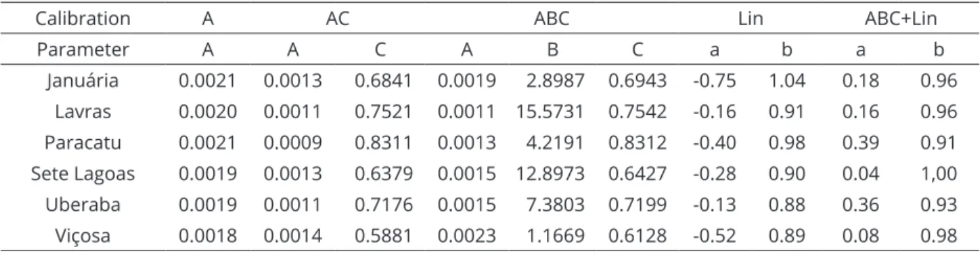
Calibration A AC ABC Lin ABC+Lin

Parameter A A C A B C a b a b

Januária 0.0021 0.0013 0.6841 0.0019 2.8987 0.6943 -0.75 1.04 0.18 0.96

Lavras 0.0020 0.0011 0.7521 0.0011 15.5731 0.7542 -0.16 0.91 0.16 0.96

Paracatu 0.0021 0.0009 0.8311 0.0013 4.2191 0.8312 -0.40 0.98 0.39 0.91

Sete Lagoas 0.0019 0.0013 0.6379 0.0015 12.8973 0.6427 -0.28 0.90 0.04 1,00

Uberaba 0.0019 0.0011 0.7176 0.0015 7.3803 0.7199 -0.13 0.88 0.36 0.93

Viçosa 0.0018 0.0014 0.5881 0.0023 1.1669 0.6128 -0.52 0.89 0.08 0.98

RESULTS AND DISCUSSION

When only the parameter “A” was calibrated (calibration A), its value varied from 0.0018 (Viçosa) to 0.0021 (Januária and Paracatu), values lower than the original

Table 4: Empirical parameters of the calibrated Hargreaves-Samani equation (A, B and C) and calibration

parameters obtained by linear regression (a, b).

(0.0023), which indicate that the original equation has a tendency to overestimate reference evapotranspiration (ET_o) in the studied sites (Table 4). The present values of parameter “A” are close to those obtained by Sentelhas, Gillespie and Santos, (2010), that found variation from 0.0017 to 0.0022.

For the calibration of parameters “A” and “C” simultaneously (calibration AC) a variation from 0.0009 (Paracatu) to 0.0014 (Viçosa) for the parameter “A” and from 0.5881 (Viçosa) to 0.8311 (Paracatu) for the parameter “C” were observed (Table 4). It is important to draw attention to the fact that these parameters are strongly correlated, when one increases the other decreases and vice versa. Subsequently, a linear correlation analysis was performed and a value of -0.97 was obtained. Similar behavior was reported by Berti et al. (2014).

When the parameters “A”, “B” and “C” was simultaneously calibrated (calibration ABC), the values of parameters “A”, “B” and “C” ranged from 0.0011 to 0.0023, 1.1669 to 15.5731 and 0.6128 to 0.8312, respectively. Bogawski and Bendroz (2014) found values of 0.001, 17.0 and 0.724 for the parameters “A”, “B” and “C”, respectively (Table 4).

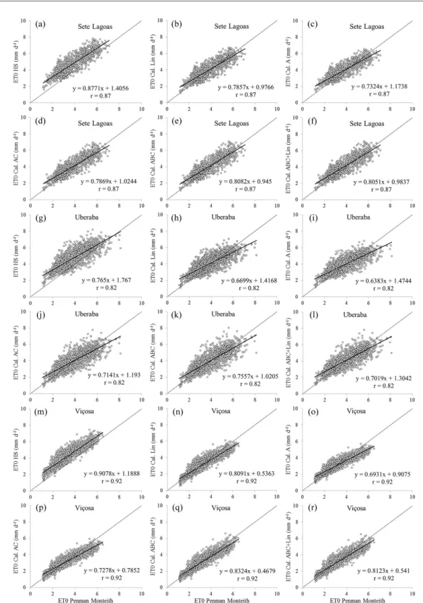
In order to facilitate the visualization of the calibrations effect, scatter plots with the ET_o values predicted by the HS equation before and after the calibrations in respect to those predicted by the PM equation were elaborated (Figures 2 and 3).

The analyzing of the Figures 2 and 3 also showed that the HS equation has a tendency to overestimate the ET_o in the studied sites, corroborating the reducing of the parameter “A” value occurred in the calibration of this parameter alone.

Analyzing the above mentioned figures could be

The performances of the Hargreaves-Samani equation (HS) not calibrated and calibrated by the different methodologies under study were evaluated also

based on the statistical indicators and classification of the

performance index presented in Table 5.

The not calibrated HS equation showed performance

classified as “good” for Januária, Paracatu, Sete Lagoas

and Uberaba and as “very good” for Lavras and Viçosa. After the calibrations, it was possible to obtain better

classifications for Lavras, Paracatu, Sete Lagoas and

Viçosa. The others (Januária and Uberaba) remained with

the same classification. Although the not calibrated HS

equation had presented a good performance the calibration is important to make the ET_o estimates even more accurate.

From the evaluation of the performance index (PI) and Willmott’s index of agreement (d) it was observed that all calibrations under study promoted an increasing of these indexes, with exception only for Paracatu with calibration A, where respectively values equal and less than those found for the not calibrated equation were obtained. It should be noted that, in most literature records, local calibration, performed in several ways, promotes better performances (Cobaner, 2011; Arraes et al., 2016; Borges Júnior et al., 2017).

Municipality Index HS Lin A AC ABC ABC+Lin

Januária MAE (mm d-1) _{0.74 0.62 0.64 0.61 0.61 0.61}

MBE (mm d-1) _{0.45 -0.08 -0.06 -0.09 -0.03 -0.03}

d 0.85 0.88 0.86 0.88 0.90 0.89

r 0.81 0.81 0.81 0.82 0.82 0.82

PI 0.69 0.72 0.70 0.72 0.74 0.73

Classification Good Good Good Good Good Good

Lavras MAE (mm d-1) _{0.62 0.47 0.48 0.44 0.44 0.44}

MBE (mm d-1) _{0.50 -0.06 -0.04 -0.12 -0.12 -0.08}

d 0.91 0.94 0.93 0.95 0.95 0.95

r 0.89 0.89 0.89 0.91 0.91 0.91

PI 0.81 0.84 0.83 0.86 0.86 0.86

Classification V. Good V. Good V. Good Great Great Great

Paracatu MAE (mm d-1) _{0.67 0.67 0.66 0.57 0.57 0.57}

MBE (mm d-1) _{0.30 -0.18 -0.13 -0.18 -0.18 -0.16}

d 0.87 0.87 0.86 0.90 0.91 0.90

r 0.80 0.80 0.80 0.84 0.85 0.85

PI 0.69 0.70 0.69 0.76 0.77 0.77

Classification Good Good Good V. Good V. Good V. Good

Sete Lagoas MAE (mm d-1) _{0.98 0.50 0.51 0.52 0.52 0.53}

MBE (mm d-1) _{0.94 0.17 0.16 0.22 0.22 0.25}

d 0.82 0.92 0.92 0.92 0.92 0.92

r 0.87 0.87 0.87 0.87 0.87 0.87

PI 0.71 0.80 0.80 0.81 0.81 0.80

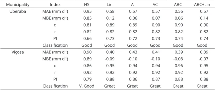
Classification Good V. Good V. Good V. Good V. Good V. Good Table 5: Statistical indexes and classification for the Hargreaves-Samani equation not calibrated (HS) and

calibrated by linear regression (Lin), adjustment of parameter “A” (A), adjustment of parameters “A” and “C” (AC), adjustment of parameters “A”, “B” and “C” (ABC) and adjustment of parameters “A”, “B” and “C” followed by calibration by linear regression (ABC+Lin).

In general, the highest values of PI and d were obtained for the calibration ABC. However, all the other calibrations also produced close values for these indexes, especially the calibrations ABC+Lin and the calibration AC. The calibration A obtained the lowest values.

As observed for the PI and d, for the mean absolute error (MAE), it was verified that all the calibrations promoted better values (lower values), leading to more

efficient ETo estimates. The calibrations AC, ABC and

ABC+Lin were, overall, the most efficient in the reducing

of this error.

Lima Junior et al. (2016), working with calibration of parameter “A” alone and parameters “A” and “C” simultaneously, concluded that the second option promoted better results. Lee (2010) concluded that the calibration of parameters “A”, “B” and “C” simultaneously is, in general, better than the calibration of parameter “A” alone. Both aforementioned results corroborate with the present study.

In relation to the correlation coefficient (r), it was verified that the linear calibration and the calibration

A cannot change its value. This occurs because the proceeded mathematical operations affect the model linearly, changing the values of ET_o without change the correlation. On the other hand, the calibrations AC, ABC and ABC+Lin were capable to produce slight improvements in the r, highlighting Paracatu, where the two last calibrations promoted an increase from 0.80 to 0.85. Thus, in cases of low correlation, even after a calibration by linear regression, good results cannot be found (Cunha; Magalhães; Castro 2013).

Analyzing the mean bias error (MBE) it was

observed that all the calibrations promoted a significant

reduction in its value in module, reducing the tendency to overestimate or underestimate reference evapotranspiration (ET_o). According to Shahidian et al. (2013) the MBE is an important indicator because it represents a systematic under or overestimation of the predicted values. The most

efficient calibration to reduce MBE varied among the

studied municipalities. However, all the methods had a

close efficiency.

In view of the found results, the calibration ABC presented a greater potential for calibration of the HS equation, since it promoted ET_o estimates closer to those estimated by the PM equation. However, the others evaluated calibrations methods also had a near performance.

Was also verified that the calibration by linear regression performed after the calibration ABC did not improve the performance in respect to the calibration ABC.

The calibration by linear regression and the calibration A showed very close results, with a slight better performance for the first alternative. It happens because the calibration by linear regression works similar to the calibration A, given that the

multiplication of the ET_o calculated by HS by the

parameter of linear calibration “b” is equivalent to the calibration of the empirical parameter “A”. However, the calibration by linear regression also have the intercept term “a”, what can contribute to achieve a better calibration.

Municipality Index HS Lin A AC ABC ABC+Lin

Uberaba MAE (mm d-1) _{0.95 0.58 0.57 0.57 0.56 0.57}

MBE (mm d-1) _{0.85 0.12 0.06 0.07 0.06 0.14}

d 0.81 0.89 0.89 0.90 0.90 0.90

r 0.82 0.82 0.82 0.82 0.82 0.82

PI 0.66 0.73 0.72 0.73 0.74 0.74

Classification Good Good Good Good Good Good

Viçosa MAE (mm d-1) _{0.90 0.40 0.43 0.41 0.39 0.39}

MBE (mm d-1) _{0.89 -0.09 -0.10 -0.10 -0.08 -0.07}

d 0.86 0.95 0.94 0.94 0.96 0.95

r 0.92 0.92 0.92 0.92 0.92 0.92

PI 0.79 0.88 0.86 0.87 0.88 0.88

CONCLUSIONS

The original Hargreaves-Samani equation presented a variable performance among the studied sites and presented a tendency to overestimate reference evapotranspiration. After its calibration, with any of the studied methodologies, better performances were observed. The simultaneous adjustment of all the empirical parameters (A, B and C) was the best alternative for calibration of the Hargreaves-Samani equation. However, the simultaneous adjustment of the parameters A and C presented almost the same performance. The calibration by simple linear regression performed after calibrate the empirical parameters A, B e C simultaneously did not promote performance gains.

ACKNOWLEDGEMENTS

To the National Council for Scientific and Technological Development (CNPq) for granting scholarship for the first authorship and to the State Research Support Foundation of Minas Gerais State

(FAPEMIG) for the financial support.

REFERENCES

ALLEN, R. G. et al. Crop Evapotranspiration: Guidelines for computing crop water requirements.Rome:FAO Irrigation and Drainage Paper 56, 1998. 300p.

ALMOROX, J.; QUEJ, V. H.; MARTÍ, P. Global performance ranking of temperature-based approaches for evapotranspiration estimation considering Köppen climate classes. Journal of Hydrology, 528(1):514-522, 2015.

ARRAES, F. D. D. et al. Parametrização da equação de Hargreaves-Samani para o estado do Pernambuco-Brasil. Revista Brasileira de Agricultura Irrigada, 10(1):410-419, 2016.

BERTI, A. et al. Assessing reference evapotranspiration by the Hargreaves method in north-eastern Italy. Agricultural Water Management, 140(1):20-25, 2014.

BOGAWSKI, P.; BEDNORZ, E. Comparison and validation of selected evapotranspiration models for conditions in Poland (Central Europe). Water Resources Management, 28(14):5021-5038, 2014.

BORGES JÚNIOR, J. C. F. et al. Métodos de estimativa da evapotranspiração de referência diária para a microrregião de Garanhuns, PE. Revista Brasileira de Engenharia Agrícola e Ambiental, 16(4):380-390, 2012.

BORGES JÚNIOR, J. C. F. et al. Equação de Hargreaves-Samani calibrada em diferentes bases temporais para Sete Lagoas,

MG. Engenharia na Agricultura, 25(1):38-49, 2017.

CAMARGO, Â. P. de; SENTELHAS, P. C. Avaliação do desempenho de diferentes métodos de estimativa da evapotranspiração potencial no estado de São Paulo. Revista Brasileira de Agrometeorologia, 5(1):89-97, 1997.

COBANER, M. Evapotranspiration estimation by two different

neuro-fuzzy inference systems. Journal of Hydrology,

398(3):292-302, 2011.

CUNHA, F. F. da; MAGALHÃES, F. F.; CASTRO, M. A. de. Métodos para estimativa da evapotranspiração de referência para Chapadão do Sul, MS. Engenharia na Agricultura,

21(2):159-172, 2013.

FENG, Y. et al. Calibration of Hargreaves model for reference evapotranspiration estimation in Sichuan basin of southwest China. Agricultural Water Management, 181(1):1-9, 2017.

FERNANDES, D. S. et al. Calibração regional e local da equação de Hargreaves para estimativa da evapotranspiração de referência. Revista Ciência Agronômica, 43(2):246-255, 2012.

HARGREAVES, G. H.; SAMANI, Z. A. Reference crop evapotranspiration from temperature. Applied Engineering in Agriculture, 1(2):96-99, 1985.

LEE, K. H. Relative comparison of the local recalibration of the temperature-based evapotranspiration equation for the Korea Peninsula. Journal of Irrigation and Drainage Engineering, 136(9):585-594, 2010.

LIMA JUNIOR, J. C. et al. Parametrização da equação de Hargreaves e Samani para estimativa da evapotranspiração de referência no Estado do Ceará, Brasil. Revista Ciência Agronômica, 47(3):447-454, 2016.

MAESTRE-VALERO, J. F.; MARTÍNEZ-ÁLVAREZ, V.;

GONZÁLEZ-REAL, M. M. Regionalization of the Hargreaves coefficient

to estimate long-term reference evapotranspiration series in SE Spain. Spanish Journal of Agricultural Research,

11(4):1137-1152, 2013.

MARTÍ, P. et al. Parametric expressions for the adjusted Hargreaves coefficient in Eastern Spain. Journal of Hydrology, 529(1):1713-1724, 2015.

SHAHIDIAN, S. et al. (2013). Parametric calibration of the Hargreaves-Samani equation for use at new locations. Hydrological Processes, 27(4):605-616, 2013.

SHIRI, J. et al. Independent testing for assessing the calibration of the Hargreaves-Samani equation: New heuristic alternatives for Iran. Computers and Electronics in Agriculture,

117(1):70-80, 2015.

SILVA, R. D. da et al. Reference evapotranspiration for Londrina,

Paraná, Brazil: Performance of different estimation methods. Semina: Ciências Agrárias, 38(4):2363-2374, 2017.

TODOROVIC, M.; KARIC, B.; PEREIRA, L. S. Reference evapotranspiration estimate with limited weather data across a range of Mediterranean climates. Journal of Hydrology, 481(1):166-176, 2013.

WILLMOTT, C. J. On the validation of models. Physical Geography, 2(2):184-194, 1981.

WILLMOTT, C. J.; MATSUURA, K. Advantages of the mean