Ordered Response Models for Sovereign
Debt Ratings
*António Afonso,
$ #Pedro Gomes,
+and Philipp Rother
#$ UECE – Research Unit on Complexity in Economics; Department of Economics, ISEG/TULisbon -
Technical University of Lisbon, R. Miguel Lupi 20, 1249-078 Lisbon, Portugal.
# European Central Bank, Directorate General Economics, Kaiserstraße 29, D-60311 Frankfurt am Main,
Germany
+ London School of Economics & Political Science.
Abstract
Using ordered logit and probit plus random effects ordered probit approaches, we study the determinants of sovereign debt ratings. We found that the last procedure is the best for panel data as it takes into account the additional cross-section error.
JEL: C25; E44; F30; G15
Keywords: ordered probit; ordered logit; random effects ordered probit; sovereign rating
* The opinions expressed herein are those of the authors and do not necessarily reflect those of the ECB or
1. Introduction
Sovereign debt ratings are forward-looking qualitative measures of the probability of default, given in the form of a code. As they are a qualitative ordinal measure, the most suitable approach to understand their determinants is an ordered response framework (see for example Hu et al., 2002; Bissoondoyal-Bheenick, 2005). However, this framework is not optimal in that its properties are only valid asymptotically, so if we estimate the determinants of the ratings using a cross-section of countries, we would have too few observations. Therefore, it is imperative to try to maximize the number of observations by using a panel data set. This poses its own difficulties as there is a country-specific error which makes the generalization of ordered probit and ordered logit to panel data is not completely straightforward.
We compare three possible estimation procedures suitable for panel data: ordered probit and ordered logit with a robust variance-covariance matrix, and random effects ordered probit. Although the three procedures are valid, the latter should be considered the best one for panel data as it considers the existence of an additional normally distributed cross-section error. In order to solve the possible problem of correlation of the errors and the regressors, we model the country-specific error, which in practical terms implies adding time averages of the explanatory variables as additional time-invariant regressors. Moreover, our panel data set includes information on rating notations for two of the main rating agencies (Standard & Poor’s and Moody’s), covering 66 countries between 1996 and 2005.
2. Methodology
The setting is the following. Each rating agency makes a continuous evaluation of a country’s credit worthiness, embodied in an unobserved latent variable R*
*
it it i i it
R =βX +λZ + +a µ . (1)
This latent variable has a linear form and depends on Xit, which is a vector containing
time-varying explanatory variables, and Zi, a vector of time-invariant variables.
In (1) the index i (i=1,…,N) denotes the country, the index t (t=1,…,T) indicates the period, and ai stands for the country-specific error. Additionally, it is assumed that the
disturbances µit are independent across countries and across time. To deal with possible
correlation between the variables in Xit we model the error term ai, as described in
Wooldridge (2002) and used by Hajivassiliou and Ioannides (2006). The idea is to express explicitly the correlation between the error and the regressors, stating that the expected value of the country-specific error is a linear combination of the time averages of the regressorsXi:
( | , ) i it i i
E a X Z = ηX . (2)
If we modify our initial equation (1) with ai =ηXt +εi we obtain
*
i X
it it i i it
whereεi is an error term by definition uncorrelated with the regressors. In practical terms, we eliminate the problem by including a time average of the explanatory variables as additional time-invariant regressors. We can write our full model as1
* ( X ) ( )X
i i
it it i i it
R =β X − + η β+ +λZ + +ε µ . (4)
Because there is a limited number of rating categories, the rating agencies will have several cut-off points that draw up the boundaries of each rating category. The final rating will then be given by2
* 16 * 16 15 * 15 14 * 1 it it it it it AAA if R c AA if c R c R AA if c R c CCC if c R ⎧ > ⎪ + > > ⎪⎪ =⎨ > > ⎪ ⎪ ⎪< + > ⎩ # . (5)
The parameters of equation (4) and (5), notably β, η , λ and the cut-off points c1 to c16
are estimated using maximum likelihood. Since we are working in a panel data setting, the generalization of ordered probit and ordered logit is not straightforward, because instead of having one error term, we now have two. Wooldridge (2002) describes two approaches that can be followed to estimate this model. One “quick and dirty” possibility is to assume we only have one error term that is serially correlated within countries. Under that assumption, one can either do the normal ordered probit
1 By estimating this specification one can interpret β as the short-run impact of the variable on the rating,
while (β+ η) gives the long-run effect of a change in the variable on the rating.
2 We grouped the ratings in 17 categories, by assigning linearly a value of 17 to the best rating, AAA, a
value of 2 to B- and a value of 1 to all observations below B-. If we used a specific number for each existing rating notch, it might be hard to efficiently estimate the threshold points between CCC+ and
estimation, using a robust variance-covariance matrix estimator to account for the serial correlation, or alternatively we can assume a logistic distribution. The second possibility is to use a random effects ordered probit model, which considers both errors εi and µit to
be normally distributed, and accordingly maximizes the log-likelihood. Of the two approaches, the second is the best one, although a drawback the quite cumbersome calculations involved. In what follows, we use the procedure created for STATA by Rabe-Hesketh et al. (2000) and substantially improved by Frechette (2001a, 2001b).
3. Estimation results
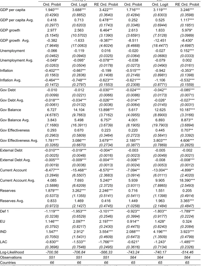
We identify the following relevant determinants of sovereign ratings: GDP per capita, real GDP growth, inflation, unemployment, government debt, the fiscal balance, government effectiveness, external debt, foreign reserves, the current account balance, default history, regional dummies and a European Union dummy. Fiscal and external stock and flow variables are used as GDP ratios. The variables of inflation, unemployment, GDP growth, the fiscal balance and the current account entered as a three-year average, reflecting the rating agencies’ approach of removing the effects of the business cycle when deciding on a sovereign rating. “Government effectiveness” is a World Bank indicator that measures the quality of public service delivery. The external debt variable was taken from the World Bank and is only available for non-industrial countries, so for non-industrial countries the value 0 has been used, which is equivalent to using a multiplicative dummy. As for the dummy variable for the European Union, the variable enters with two leads. Default history is assessed by a dummy if the country has defaulted since 1980. We also included a dummy for industrialised countries and another for Latin America and Caribbean countries. Regarding the ratings data, we use the sovereign foreign currency rating attributed by
the two main rating agencies between 1996 and 2005. Data sources comprise the rating agencies and the International Monetary Fund, the World Bank and the Inter-American Development Bank for the explanatory variables.
Table 1 reports the estimation results. In the random effects ordered probit, more variables show up as significant: seven for Moody’s, and nine for S&P. This is because the standard deviations are considerably smaller in these methods, in comparison to the other two approachs. The signs of the coefficients are consistent across the estimations.
[Insert Table 1 here]
We evaluate the performance of the three models by focusing on two elements: the prediction for the rating of each individual observation in the sample, and the prediction of movements in the ratings through time. Table 2 presents an overall summary of the prediction errors.
[Insert Table 2 here]
For Moody’s we see that the three models are quite similar in predicting the level of rating. Roughly, 45 per cent of the observations are predicted correctly, 80 per cent are predicted within a notch and 95 per cent within 2 notches. For S&P the models perform quite similarly in correctly predicting the rating, but with a higher percentage of predictions within a notch.
Let us now turn to how the models perform in predicting changes in ratings. Table 3 presents the total number of sample upgrades (downgrades), the predicted number of upgrades (downgrades) and the number of upgrades (downgrades) that were correctly predicted by the three models.
[Insert Table 3 here]
Generally, the models correctly predict half of both upgrades and downgrades in the period they actually occurred, and a third more in the following period. The most noticeable difference between the models is not the number of corrected predicted changes, but the total number of predicted changes. In fact, the ordered probit and ordered logit predict more changes than the random effects ordered probit. For instance, for Moody’s the first two models predict around 120 upgrades, whereas the random effects ordered probit only predicts 95, the actual number being 58.
4. Conclusion
We have compared three procedures to estimate the determinants of sovereign ratings under an ordered response framework: ordered probit, ordered logit and random effects ordered probit. Of the three, the most efficient method is the random effects ordered probit estimation is the more efficient method, since a considerable number of variables show up as significant that are not picked up using the other two methods. Even though in terms of predicting the ratings, all three methods show similar performance in anticipating changes in ratings, nevertheless the random effects ordered probit slightly outperforms the other two specifications.
Acknowledgements
Pedro Gomes would like to thank the Fiscal Policies Division of the ECB for its hospitality, and acknowledges the financial support of the FCT (Fundação para a Ciência e a Tecnologia, Portugal). UECE is also supported by the FCT.
References
Bissoondoyal-Bheenick, E. (2005). An analysis of the determinants of sovereign ratings. Global Finance Journal 15 (3), 251-280.
Frechette, G. (2001a). sg158: Random-effects ordered probit, Stata Technical Bulletin 59, 23-27. Reprinted in Stata Technical Bulletin Reprints 10, 261-266.
Frechette, G. (2001b). sg158.1: Update to random-effects ordered probit, Stata Technical Bulletin 61, 12. Reprinted in Stata Technical Bulletin Reprints 10, 266-267. Hajivassiliou, V. and Ioannides, Y. (2006). Unemployment and liquidity constraints. Journal of Applied Econometrics (forthcoming).
Hu, Y.-T.; Kiesel, R. and Perraudin, W. (2002). The estimation of transition matrices for sovereign credit ratings. Journal of Banking & Finance 26 (7), 1383-1406.
Rabe-Hesketh, S.; Pickles, A. and Taylor, C. (2000). sg120: Generalized linear latent and mixed models. Stata Technical Bulletin 53, 47-57. Reprinted in Stata Technical Bulletin Reprints 9, 293-307.
Wooldridge, J. (2002). Econometric Analysis of Cross Section and Panel Data. MIT Press.
Table 1 – Estimation results
Moody’s S&P
Ord. Probit Ord. Logit RE Ord. Probit Ord. Probit Ord. Logit RE Ord. Probit GDP per capita 1.940*** 3.688*** 3.422*** 1.716*** 3.119*** 3.246***
(0.4290) (0.8852) (0.3640) (0.4284) (0.8303) (0.3598)
GDP per capita Avg. 0.418 0.713 0.478*** 0.252 0.525 1.117***
(0.2977) (0.6203) (0.1743) (0.3346) (0.6944) (0.1851) GDP growth 2.977 2.563 6.464** 2.613 1.833 5.979* (5.1545) (10.5702) (3.1390) (3.6591) (7.5128) (3.0989) GDP growth Avg. -0.382 -1.633 -9.387** -8.511 -12.451 -8.430* (7.9649) (17.0063) (4.6024) (8.4668) (18.4477) (4.6987) Unemployment -0.066 -0.119 0.016 -0.020 -0.027 0.152*** (0.0462) (0.0940) (0.0325) (0.0364) (0.0680) (0.0333) Unemployment Avg. -0.049* -0.095* -0.078*** -0.038 -0.079 0.002 (0.0263) (0.0504) (0.0178) (0.0273) (0.0490) (0.0161) Inflation -0.402*** -0.667** -0.199 -0.515*** -0.942 -0.353** (0.1563) (0.2836) (0.1408) (0.2149) (0.8981) (0.1398) Inflation Avg. -0.464*** -0.748*** -0.623*** -0.621*** -1.106 -0.532*** (0.1472) (0.2797) (0.1553) (0.2308) (0.8771) (0.1559) Gov Debt -0.010 -0.012 -0.030*** -0.024*** -0.042** -0.085*** (0.0099) (0.0221) (0.0066) (0.0086) (0.0173) (0.0071)
Gov Debt Avg. -0.018*** -0.034*** -0.026*** -0.014** -0.026* -0.027***
(0.0061) (0.0132) (0.0036) (0.0064) (0.0145) (0.0031)
Gov Balance 6.727 14.104 13.898*** 5.617 12.625 10.187***
(4.6787) (9.7663) (3.7162) (4.0955) (8.8900) (3.3166)
Gov Balance Avg. 3.843 5.498 6.757* 4.001 6.893 8.873**
(7.1680) (16.3911) (3.6739) (8.1905) (19.7903) (3.6894)
Gov Effectiveness 0.293 0.670 0.223 0.220 0.445 0.707**
(0.2963) (0.5809) (0.3464) (0.2723) (0.5641) (0.3392)
Gov Effectiveness Avg. 1.781*** 3.086*** 3.679*** 2.185*** 3.803*** 4.606***
(0.3265) (0.6670) (0.2734) (0.3877) (0.7869) (0.2825)
External Debt -0.010*** -0.019*** -0.004** -0.003 -0.005 -0.002
(0.0025) (0.0048) (0.0016) (0.0023) (0.0049) (0.0021)
External Debt Avg. -0.005*** -0.009*** -0.004*** -0.006** -0.008 -0.008***
(0.0019) (0.0036) (0.0013) (0.0024) (0.0053) (0.0012)
Current Account -8.477*** -15.468** -8.570*** -7.094** -13.004** -4.899**
(3.2849) (6.5507) (2.3683) (3.0914) (6.0111) (2.4020)
Current Account Avg. 4.085 7.693 5.240** 5.939 9.905 18.390***
(3.5886) (6.6209) (2.3725) (3.9311) (7.8865) (2.5493) Reserves 1.879*** 3.262*** 2.246*** 0.716 1.551 0.205 (0.5373) (1.1355) (0.5141) (0.5411) (1.1398) (0.4914) Reserves Avg. 0.833 1.469 0.416 1.449 1.963 3.365*** (0.9723) (2.1427) (0.4745) (1.0258) (2.1484) (0.4847) Def 1 -1.119*** -1.953*** -3.101*** -0.923** -1.803** -1.789*** (0.3238) (0.6529) (0.2546) (0.3994) (0.9177) (0.2224) EU 1.146*** 2.097** 2.197*** 0.914** 1.428* 0.324 (0.3792) (0.8217) (0.2430) (0.4475) (0.8240) (0.2084) IND 1.547** 2.912* 3.554*** 2.088*** 4.196*** 3.923*** (0.7050) (1.5431) (0.4609) (0.6473) (1.3509) (0.4799) LAC -0.830** -1.533** -1.766*** -0.621* -1.243* -1.485*** (0.3696) (0.7548) (0.2495) (0.3616) (0.7134) (0.2326) Log-Likelihood -700.56 -706.84 -566.33 -743.24 -740.17 -514.46 Observations 551 551 551 564 564 564 Countries 66 66 66 65 65 65
Notes: The standard deviations are in parentheses. *, **, *** - statistically significant at the 10, 5, and 1 per cent. When estimating (4) the variables enter the estimation as differences from the country average. An additional regressor for each variable, which represents the time-average within a country, is represented with Avg.
Table 2 – Summary of prediction errors
Notes: * prediction error within +/- 1 notch. ** prediction error within +/- 2 notches.
Table 3 – Upgrades and downgrades prediction Prediction error (notches)
Estimation
Procedure Obs. 5 4 3 2 1 0 -1 -2 -3 -4 -5 % Correctly predicted % Within 1 notch * % Within 2 notches ** Ordered Probit 551 1 5 12 39 92 259 88 50 5 0 0 47.0% 79.7% 95.8% Ordered Logit 551 5 2 13 35 98 259 90 45 4 0 0 47.0% 81.1% 95.6% Moody’s RE Ordered Probit 551 0 8 20 43 104 258 74 28 15 1 0 46.8% 79.1% 92.0% Ordered Probit 564 0 4 18 25 110 251 117 28 11 0 0 44.5% 84.8% 94.1% Ordered Logit 564 0 6 18 17 115 257 116 26 9 0 0 45.6% 86.5% 94.1% S&P RE Ordered Probit 564 1 3 19 38 111 204 147 35 6 0 0 36.2% 81.9% 94.9% Upgrades correctly predicted at time Downgrades correctly predicted at time Sample Upgrades Predicted Upgrades t t+1 Sample Downgrades Predicted Downgrades t t+1 Ordered Probit 58 119 25 18 34 70 17 10 Ordered Logit 58 122 25 21 34 73 17 11 Moody’s RE Ordered Probit 58 95 25 16 34 61 16 8 Ordered Probit 79 105 34 16 41 72 18 16 Ordered Logit 79 105 38 20 41 71 20 14 S&P RE Ordered Probit 79 102 35 20 41 66 18 12