Combustion analysis on a CFM56-3 engine

UNIVERSIDADE DA BEIRA INTERIOR

Engenharia

Combustion analysis on a CFM56-3 engine

Kevin Azevedo das Neves

Dissertação para obtenção do Grau de Mestre em

Engenharia Aeronáutica

(Ciclo de estudos integrado)

Orientador: Prof. Doutor Francisco Miguel Ribeiro Proença Brojo

Dedication

To my beloved parents, Patrocínia and Fernando Neves, who have always been an inspiration and to whom I owe everything.

To my brother and sister, Lucas and Melisa, who I unconditionally love and to whom I wish the brightest future.

A smooth sea never made a skilled sailor.

Acknowledments

I would like to thank my family who have always supported me and gave me freedom to persue my dreams. All the goals I have accomplished so far and the person I stand today are due to your inconditional care.

A big thank you to my supervisor, Professor Francisco Brojo, who have always kept me in the right path during this challenging time. I will always be grateful for your guidance and constant support. I can not describe how grateful I am for the availability and promptitude when I needed help.

I am deeply grateful to my Executive Board of AIESEC in Covilhã UBI, who I can not be more honored to have had the opportunity to lead during the last year. Patrícia, Alexandre and Maria, you embraced this huge challenge with me and I can not thank you enough for helping me evolving our committee to a whole new level. With you, I learned so much and I spent some of the greatest moments of this year.

For all AAUBI 2017 team, I want to thank you for all the opportunities I had with you and for each memorable moment I will never forget. Thank you for being able to really take an active role in the improvement of our students community.

I am profoundly grateful to my dearest friend Robert Gonçalves, who have raised this passion for aeronautics in me, and who was always a great companion to talk to during the last five years.

Last but not least, I would like to thank all my friends from Pombal, Belo Horizonte and Covilhã, specially to Rafael, who made my academic experience unique.

Resumo

Quanto mais eficiente um motor é, menos combustível é necessário para ir de um ponto A para um ponto B e menos gases de efeito estufa são produzidos. Apesar de serem uma fonte de dióxido de carbono significante, os motores de turbina de gás lideram os sistemas de propulsão aeronáutica e provavelmente assim vão continuar nas próximas décadas. Portanto, uma das formas mais rápidas de procurar ser sustentável nos céus é melhorando a sua

performance. Todavia, estes motores representam um dos mais complexos problemas de

engenharia, uma vez que dependem de centenas de diferentes parâmetros que ao variarem podem levar a que surja uma configuração melhor. No entanto, disponibilizamos de computadores e softwares capazes de testar diferentes conceitos. Este trabalho consistiu em uma análise numérica da combustão de Jet-A no combustor anular do CFM56-3, através de dois modelos de turbulência diferentes. A geometria utilizada foi ¼ do motor construído pelo Jonas Oliveira, ao realizer um scan 3D a um combustor real. Esta geometria foi importada para um software de CFD, CONVERGE Studio, onde todos os parâmetros dos ensaios foram configurados. A simulação em sim foi realizada no software principal CONVERGE, instalado num computador de alto desempenho. O objetivo final deste estudo passou pela comparação do comportamento de cada modelo de turbulência, enquanto estudamos a performance de um dos mais populares motores turbofan. Os modelos de turbulência escolhidos foram o

standard 𝑘-𝜀 e o standard 𝑘-𝜔, para além de ter sido selecionado um conjunto de modelos

para simular a injeção de combustível através de vaporização, de modo a prever melhor o comportamento do escoamento dentro do combustor. De forma a comparar estes modelos, seis parâmetros principais foram analisados: a enregia cinética turbulenta (𝑘); a taxa de dissipação da energia cinética turbulenta (𝜀); a dissipação da energia cinética turbulenta

específica (𝜔); o comprimento característico dos turbilhões (𝑙); a velocidade de fricção (𝑢∗_);

e a distãncia adimensional à parede (𝑦+_{). Ambos os modelos mostraram um comportamento}

semelhante ao longo do tempo para todos os parâmetros. Todos os resultados encontram-se na mesma ordem de grandeza, apesar apresentarem uma diferença considerável no seu valor absoluto. Os mesmos foram considerados aceitáveis, após uma comparação quantitativa com parâmetros à saída do combustor e uma comparação qualitativa de um perfil de temperaturas e de um perfil de energia cinética turbulenta com dois estudos de configurações similares. Por fim, nenhum modelo foi classificado melhor que o outro, devido à complexidade envolvida num estudo deste tipo, mas apenas considerados diferentes.

Palavras-chave

Combustão; Turbulência; Modelo; CFM56-3; Jet-A; CFD; CONVERGE.

Abstract

The more fuel efficient an engine is, the less fuel is needed to get from point A to point B and the less Greenhouse gases will be produced. In spite of being a major source of carbon dioxide, gas turbine engines lead the aircraft propulsion systems globally and will probably continue for the next decades. Thus, one of the most immediate ways to go green on the skies is by advancing their performance. Nontheless, GTE’s are one of the most complex engineering problems, as they rely on hundreds of parameters that can be tweaked and result in a better configuration. However, we have computers and softwares that allow us to test engine concepts. This study consisted in a numerical analyses of the combustion of Jet-A in the annular combustor of the CFM56-3 engine, through two different turbulence models. The geometry used was ¼ of the engine constructed by Jonas Oliveira by performing a 3D scan on a real size combustor. This geometry was imported and prepared in a CFD software, CONVERGE Studio, where the case setup was configured. The simulation itself was run on the main software CONVERGE installed on a multi-core high performance machine. The final goal of this study was to compare the behavior of each turbulence model when studying the performance of annular combustors similar to the most popular turbofan engine’s. The turbulence models chosen were the standard 𝑘-𝜀 and the standard 𝑘-𝜔 and also a set of models were defined to simulate the injection of fuel through a parcel spray and, therefore, better predict the flow inside the combustor. To compare the simulation results, six main parameters were analysed: Turbulent Kinematic Energy (𝑘); Turbulence Dissipation Rate (𝜀); Specific Turbulence Dissipation Rate (𝜔); Turbulent Length Scale (𝑙); Friction Velocity (𝑢∗_);

and the dimensionless wall distance (𝑦+_{). Both models demonstrated a similar behavior in all}

the parameters, along the runtime. The results were all within the same order of magnitude, although the absolute values have shown a considerable difference. The simulation outputs were considered acceptable after comparing quantitatively the exhaust parameters, and qualitatively a temperature and TKE contour with two previous works with similar setup conditions. Any turbulence model was judged better than the other, due to the complexity involved in such a study, but only considered different.

Keywords

Contents

2 Two equation Models 17

2.1 𝑘-𝜀 Model 17

2.2 𝑘-𝜔 Model 19

2.3 Comparisation of the Two-equation Models in diverse applications 20

3 Combustion Considerations 21

3.1 Stoichiometry 23

3.2 Absolute Enthalpy, Enthalpy of Formation and Enthalpy of Combustion 23

3.3 Adiabatic Flame Temperature 24

3.4 Combustion Modeling 25

4 CFM56-3 27

4.1 The Combustion Chamber 28

4.2 Fuel Injection 30

4.2.1 Fuel Spray Nozzle 30

4.3 Ignition System 32 4.3.1 Spark Igniters 32 5 Problem Modeling 35 5.1 Surface Preperation 36 5.2.1 Importing .stl files 37 5.2.2 Defining Boundaries 37 5.2.3 Geometry Defects 38 5.2 Case Setup 39 5.2.1 Materials 39 5.2.2 Simulation Parameters 40 5.2.3 Boundary Conditions 40

5.2.4 Regions and Initialization 42

5.2.6 Grid Control 44

5.2.7 Output/Post Processing 45

6 Results 47

6.1 Results Validation 48

6.2 Turbulence Models Analysis 49

6.3 Conclusion 53

6.4 Future Studies 55

Bibliography 57

List of Figures

Figure 1.1 – Turbulence modelling approaches and their applications 7

Figure 1.2 – Energy cascade spectrum 13

Figure 1.2 – Typical turbulent boundary layer velocity profile 16

Figure 3.1 – Primary energy Comsumption in 2015 21

Figure 3.2 – Flame mode of combustion in a spark-ignition engine 22

Figure 3.3 – Non flame mode of combustion in a spark-ignition engine 22

Figure 4.1 – CFM56-3 schematic 28

Figure 4.2 – Combustion Chamber 29

Figure 4.3 – Flows in the Combustion Chamber 30

Figure 4.4 – Fuel Nozzle installation 31

Figure 4.5 – Fuel Nozzle cross section 31

Figure 4.6 – Dual orifice spray tip 32

Figure 4.7 - Spark Plug 33

Figure 5.1 – CONVERGE workflow 36

Figure 5.2 – Detailed view of triangles assigned to different boundaries 37

Figure 5.3 – Triangles assigned to different boundaries distinguished by colors 38

Figure 5.4 – Example of defects arisen by conflict between two boundaries 39

Figure 5.5 - Injector with a single nozzle spraying a solid 10 degree cone shape 43

Figure 5.6 - Spray rate of fuel throughout the simulation runtime in each injector 44

Figure 6.1 - Average exhaust flow temperature 48

Figure 6.2 - Temperature contours 49

Figure 6.3 – Turbulent Kinetic Energy contours 50

Figure 6.4 - Turbulent Kinetic Energy (𝑘) results from 𝑘-𝜀 and 𝑘-𝜔 models 51

Figure 6.5 - Turbulent Dissipation Rate (𝜀) results from 𝑘-𝜀 and 𝑘-𝜔 models 51

Figure 6.6 – Specific Turbulent Dissipation Rate (𝜔) results from 𝑘-𝜀 and 𝑘-𝜔 models 52

Figure 6.7 - Length Scale (𝑙) results from 𝑘-𝜀 and 𝑘-𝜔 models 52

Figure 6.8 - Friction Velocity near the walls (𝑢∗_{) from 𝑘-𝜀 and 𝑘-𝜔 models 52}

Figure 6.9 - Dimensionless wall distance (𝑦+_{) results 53}

List of Tables

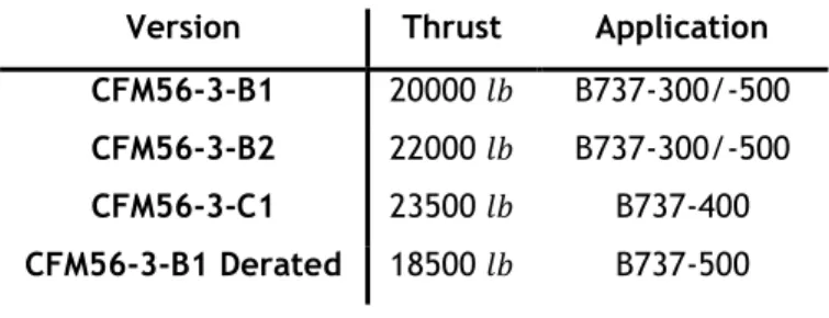
Table 4.1 – CFM56-3 versions, thrust and application 27

Table 5.1 – Type and number of defects found on the geometry surface 38

Table 5.2 – Global transport parameters 40

Table 5.3 – Simulation parameters 40

Table 5.4 – Input values for air mass flow of each boundary, while burning Jet-A at full

power 41

Table 5.5 – Output variables chosen 45

Table 5.6 – CONVERGE frequency of writing data files 46

Table A.1 - Relevant data form Pedro’s work 61

List of Acronyms

AFR Air to Fuel Ratio

AMR Adaptive mesh Refinment

ASCII American Standard Code for Information Interchange

ASM Algebraic Stress Model

CEQ Chemical EQuilibrium

CFD Computational Fluid Dynamics

CTC Characteristic Time Combustion

DNS Direct Numerical Simulation

ECFM Extended Coherent Flame Model

FGM Flamelet Generated Manifold

GHG Green House Gases

GTE Gas Turbine Engine

HPC High Pressure Compressor

HPT High Pressure Turbine

ICAO International Civil Aviation Organization

LES Large Eddy Simulation

PZ Primary Zone

RAM Random Access Memory

RANS Reynolds-Averaged Navier-Stokes

RIF Representative Interactive Flamelet

RNG Re-Normalisation Group

RSM Reynolds Stress Model

SAS Scale-Adaptive Simulation

SGS Sub Grid Scale

SST Shear Stress Transport

SZ Secondary Zone

TAP Transportes Aéreos de Portugal

TKE Turbulent Kinetic Energy

Nomenclature

𝐴 Area [𝑚2]

𝐵 Wall roughness constant [−]

𝐶𝜀1 𝑘-𝜀 model constant [−] 𝐶𝜀2 𝑘-𝜀 model constant [−] 𝐶𝜇 𝑘-𝜀 model constant [−] 𝐶𝜀1 𝑘-𝜀 model constant [−] 𝐶𝑆 Smagorinsky constant [−] 𝑓𝛽 𝑘-𝜔 model constant [−] 𝑓𝛽∗ 𝑘-𝜔 model constant [−] ℎ Absolute enthalpy [𝐽/𝑘𝑔] ℎ𝑓 Enthalpy of formation [𝐽/𝑘𝑔] Δℎ𝑟 Enthalpy of combustion [𝐽/𝑘𝑔] 𝑚 Mass [𝑘𝑔]

𝑚̇ Mass flow rate [𝑘𝑔/𝑠]

𝑘 Turbulent kinematic energy [𝑚2/𝑠2_]

𝑙 Lenghtscale [𝑚]

𝑙0 Lenghtscale of the largest eddies [𝑚]

𝑙𝐸𝐼

Demarcation lengthscale between the

energy-containing and smaller eddies [𝑚]

𝑝 Pressure [𝑃𝑎]

𝑃 Time-averaged pressure [𝑃𝑎]

𝑞 Heat [𝐽]

𝑅𝑒 Reynolds number [−]

𝑠 Strain-rate tensor [𝑁 𝑚⁄ 2. 𝑠]

𝑆 Mean strain-rate tensor [𝑁 𝑚⁄ 2. 𝑠]

𝑡 Time [𝑠]

𝑇 Temperature [K]

𝑢 Velocity [𝑚/𝑠]

𝑢+ _{Dimensionless Velocity [−]}

𝑢∗ Friction velocity [𝑚/𝑠]

𝑢𝜂 Kolmogorov velocity scale [𝑚/𝑠]

𝑈 Time-averaged velocity [𝑚/𝑠]

𝑦+ _{Dimensionless Wall distance} [−]

Greek letters 𝛼 𝑘-𝜔 model constant [−] 𝛽 𝑘-𝜔 model constant [−] 𝛽∗ _{𝑘-𝜔 model constant} [−] 𝛽𝑜 𝑘-𝜔 model constant [−] 𝛽𝑜∗ 𝑘-𝜔 model constant [−] 𝛿 Boundary-layer thickness [𝑚]

𝜀 Turbulent dissipation rate [𝑚2/𝑠3_]

𝜅 Karman constant [−]

𝜇 Absolute viscosity [𝑃𝑎. 𝑠]

𝜇𝑡 Molecular eddy viscosity [𝑃𝑎. 𝑠]

𝜈 Kinematic viscosity [𝑚2/𝑠]

𝜈𝑇 Kinematic eddy viscosity [𝑚

2_/𝑠] 𝜌 Density [𝑘𝑔/𝑚3] 𝜎 𝑘-𝜔 model constant [−] 𝜎∗ _{𝑘-𝜔 model constant} [−] 𝜎𝑘 𝑘-𝜀 model constant [−] 𝜎𝜀 𝑘-𝜀 model constant [−] 𝜏𝜂 Kolmogorov timescale [𝑠] 𝜏𝑖𝑗 Stress tensor [𝑁/𝑚 2_]

𝜔 Specific turbulent dissipation rate [1/𝑠]

Upper-case Greek Δ Filter width [𝑚] Subscripts a Air ad Adiabatic f Fuel prod Products reac Reactants ref Reference t Turbulent i, j Coordinate directions

Chapter 1

Introduction

1.1 Motivation

The most popular and commode way to go from point A to point B, if we are speaking about long distances, is by airplane. Today, most of the aircrafts use combustion to power its engines. Combustion has been present on aviation almost since the beginning of its history. It was in 1903, after four years of experimental work with gliders, that the Wright brothers flew for the first time with their heavier-than-air craft, which was powered by a 12 ℎ𝑝 (8.9 𝑘𝑊) engine [1]. It was a four-cylinder, water-cooled, internal-combustion and first gasoline engine to fly designed by themselves. The aircraft propulsion has come a long way since then, and the current state-of-the-art CFM56 turbofan engine family is the proof of the disruptive evolution. And not only it has the potential to go further, but also need to go further, once gas engines will be in our airplanes for next decades. The World Energy Council states on its 2016 Resources Report that oil remained the world’s leading fuel, accounting for 32.9% of global energy consumption; roughly 63% of oil consumption is from the transport sector. Oil substitution is not yet imminent and is not expected to reach more than 5% for the next five years [2]. Hence, one of the most immediate ways to go green on the skies is by advancing gas turbine engines. Carbon dioxide is one of the major sources of Greenhouse Gases.

Besides, CO2, along with water vapor is also the product of a complete combustion. So, the

more fuel efficient our engine is, the less fuel is needed to get from point A to point B and the less carbon dioxide will be produced.

We have made significant strides in fuel efficiency, the average fuel burn of a new aircraft fell by about 45% from 1968 to 2014 [3] and we will keep improving in order to keep up with regulations and ICAO’s technology goals. We have been able to reduce emissions and improve fuel efficiency by innovating. However, before we discuss how we can innovate in gas turbine engines, we need to understand how such engines work. A jet engine keeps an aircraft moving forward using a very simple principle. The same that makes an air filled balloon move: Newton’s 3rd law of motion. Just like the reaction force produced by the air moves the balloon, the reaction force produced by the high speed jet at the tail of the engine makes it move forward. Thus, the working of a jet engine is all about a high speed jet at the exit. The higher the speed of the jet, the greater the thrust force. Such high-speed exhaust is achieved by a combination of techniques. By heating the incoming air to a high temperature, it will

expand tremendously and will create the high velocity jet. For this purpose, a combustion chamber is used where an atomized form of the fuel is burnt inside. Effective combustion requires air to be at moderately high temperature and pressure. To bring the air to this condition, a set of compressor stages is used. The rotating blades of the compressor add energy to the fluid and its temperature and pressure rise to a level suitable to sustain combustion. A compressor receives the energy for the rotation from a turbine, which is placed right after the combustion chamber. The compressor and turbine are attached to same shaft. The high-energy fluid that leaves the chamber makes the turbine blades turn. As the turbine absorbs energy from the fluid, its pressure drops. Also, the engine case becomes narrower towards the outlet, which results in even greater jet velocity. In short, the synchronized of the compressor, combustion chamber and turbine makes the aircraft move forward. A revolutionary improvement was made by fitting a large fan with a low pressure spool and a low pressure turbine, giving rise to the what we call today turbofan engines. Almost every commercial aircraft runs on them nowadays, being the CFM56 family, a popular example. In these engines, some of the incoming air passes through the fan and continues on into the core compressor and then the burner, where it is mixed with fuel and combustion occurs. The hot exhaust passes through the core and fan turbines and then out the nozzle, as in a basic turbojet. The rest of the incoming air passes through the fan and bypasses, or goes around the engine, just like the air through a propeller. The ratio of the air that goes around the engine to the air that goes through the core is called the bypass ratio. In an engine with a bypass ratio of 5:1, for every 6 units of air drawn into the engine, 5 will bypass the engine core and 1 will go through it. In a turbofan engine, the majority of the thrust force comes from the fans reaction force. The fan greatly improves airflow in the system by absorbing more air, improving the thrust. This means, high thrust creation with an expense of slightly more fuel is the reason why turbofan engines are highly fuel economical. This better fuel economy, together with quieter exhaust, are responsible for the domination of the aircraft propulsion systems by these engines. Gas turbine engines are one of the most complex engineering problems out there. It relies on turbulent flow, fuel injection, fuel properties, fuel chemistry, fuel spray, combustion chamber, among many others. There are literally hundreds of parameters that can be tweaked in an engine to come up with an optimal configuration. Although, the greenest engine, which is our goal, is this optimal combination and we need to find it.

Finding that is not easy, once we can not build and test engines for all the combination of parameters. However, we have computers and softwares that allow us to test engine concepts before we build them. And we have optimization software that allow us to run a reduced set of designs in order to find an optimum. These tools, along with experiments have helped to meet emissions and fuel economy mandates throughout regulation history. The engines keep improving, partly because airlines want to fill up their tanks less often, but also because the regulations are forcing engine makers to find solutions in order to keep selling

aircrafts. The computer softwares we have to simulate these engines before building them are really advanced, but far from perfect under a lot of conditions and it takes a long time to run. Computer methods and speeds both need to improve significantly to get us better answers quicker, but it is worth the effort as it is an important key to allow us to go greener.

1.2 Main Goal

The present work consists in a numerical analyses of the combustion of Jet-A in the annular combustor of the CFM56-3 engine, through two different turbulence models. The geometry used was ¼ of the engine constructed by Jonas Oliveira [4] by performing a 3D scan on a real size combustor, gently provided by TAP, in which all the measurements were extracted to conduct a Computer Assisted Design with the commercial software CATIA V5. This geometry was imported to a Computer Fluid Dynamics software, CONVERGE Studio, where the case setup was configured. Then, the simulation was run on the main software CONVERGE installed on a multi-Core High Performance computer. After the simulation, the results were visualized and post-processed in CONVERGE Studio.

The turbulence models chosen were the Standard 𝑘-𝜀 and the Standard 𝑘-𝜔. As we can not

claim that any model is better than another, once it depends on the case, the author decided to use the first one giving the fact that it is the most commonly used in engineering problems and which presents better behaviours for a bigger variety of flows [5]. The second choice is also popular in performing CFD computations, once this model can be integrated near a wall without the aid of wall functions [5].

The final goal of this study is to compare the behavior of each turbulence model when studying the performance of annular combustors similar to the most popular turbofan engine’s.

1.3 Task Overview

In the first chapter, the author introduces his work by manifesting his motivation behind the development of a study with the CFM56-3 annular combustor chamber. Current issues are presented and how they are tending for the next decades, as well as the present-day resources that can be exploited to leverage this tendencies. The fundamental goals are proposed, as well as the main drivers that will conduct the study. Historical and bibliographic data is reviewed in order to have a context about the subject and its relevance nowadays. The second chapter approaches the main topics needed to better understand this work. The author introduces the combustion notions, the CFM56-3 engine and the Standard 𝑘-𝜀 and the

Standard 𝑘-𝜔 turbulence models, as they are the fundamental concepts needed to develop

the present analysis.

In the third chapter, the author presents the case setup. Here, all the parameters used on the simulations are set: applications, materials, boundary conditions, initial conditions, physical models and grid control.

The final chapter presents the numerical results of the CFD simulation. Outputs are described in detail and discussed. The chapter ends with the conclusions of this study and possible future work proposals.

1.4 Historical Review

Boussinesq performed the first attempts to develop a mathematical description of the turbulent stresses back in 1877, by introducing the eddy viscosity concept [6]. Later, in 1895, Reynolds published his research on turbulence with the time-averaged Navier-Stokes equations [7]. However, neither of the authors tried to solve this equations in any type of systematic way. In 1904, Prandtl discovers the boundary layer, which brought much more information regarding the physics of viscous flow [8]. Later, he presents the concept of the mixing-length model that established an algebraic relation for the turbulent stresses [9]. This model is now also known as zero-equation model.

Twenty years later, Prandtl came out with the first one-equation model by considering the effects of flow history, stating that the eddy viscosity depended on the turbulent kinetic energy, 𝑘 [10]. This was a more realistic mathematical model, in which a differential equation was solved to approximate the exact equation for 𝑘. Also, in 1942, Kolmogorov proposed the first complete turbulence model, taking into account the turbulent kinetic energy, 𝑘, and considering a new parameter, regarding the rate of dissipation of energy per unit volume and time, 𝜔. This model consisted in solving a differential equation for 𝜔, similarly to the solution for k. Named 𝑘-𝜔, it used reciprocal of 𝜔 as the turbulence time scale and the quantity 𝑘1/2_{⁄𝜔 as the turbulence length scale [11]. This model remained}

virtually until the emergence of computing capacity, due to the complexity required to solve nonlinear differential equations.

In 1951, Rotta used a new approach named second-order or second-moment closure, which took the Boussinesq approximation in turbulence models to solve for the Reynolds stresses, incorporating non-local and history effects, such as streamline curvature and body forces. It was a seven-equation model, using one equation for turbulence length scale and six for the Reynolds stresses. Once again, its use remained not practical until the computer technology evolved [12].

By the 1960’s, along with the computer capabilities development, these four classes of turbulence models evolved. Regarding zero-equation models, Van Driest introduced in 1956 a viscous damping correction for the mixing-length model, which is still used in the majority of the modern models [13]. In 1974, Cebeci and Smith refined the concept of mixing-length when used with attached boundary layers [14]. By 1978, Baldwin and Lomax also suggested a different algebraic zero-equation model which allowed to define a turbulence length scale from the shear-layer thickness more easily [15].

Concerning the one-equation models, they didn’t have much success, despite being much simpler than two-equation models. Bradshaw, Ferriss, and Atwell, however, formulated a model [16] which was tested against the latest experimental data at the 1968 Turbulent Boundary Layers Conference, in Stanford and is still used as it can be easily solved numerically. In turn, after Kolmogorov’s 𝑘-𝜔 model, Daly and Harlow, in 1970 [17], and Launder and Spalding, in 1972 [18], extended the study in two-equation models, giving rise to the 𝑘-𝜀 model in 1974, in which 𝜀 is the dissipation rate of turbulent kinetic energy [19]. Also, in 1970, Saffman proposed a 𝑘-𝜔 model, which revealed some advantages by integrating through the viscous sublayer and in flows with adverse pressure gradients [20]. Regarding second-order closure models, they do not have the same popularity because of their complexity. Notable studies for this class of models have been done though. For instance, Donaldson and Rosenbaum in 1968 [21] and Launder, Reece and Rodi in 1975 [22]. Also, other authors such as Lumley in 1978 [23], Speziale in 1985 [24] and 1987 [25] and Reynolds in 1987 [26] brought more mathematical rigor to the model formulation.

1.5 Bibliographic Review

Turbulence

Almost all fluid flows present in our daily life are turbulent. We can find them around cars, airplanes, buildings or in the locomotion of water, land and air living beings. Flows in rivers, oceans and atmosphere are large scale examples. Even the blood in the aorta is occasionally turbulent. A technical example is the flow and combustion of piston engines and gas turbine, which are highly turbulent and is used as a plus to help the mixing of fuel with oxidant for a more efficient combustion. There is no specific definition for turbulence. Peter Bradshaw, in

An introduction To turbulence and its Measurements states that “Turbulence is a

three-dimensional time-dependent motion in which vortex stretching causes velocity fluctuations to spread to all wavelengths between a minimum determined by viscous forces and a maximum determined by the boundary conditions of the flow. It is the usual state of fluid motion except at low Reynolds numbers” [27]. Although we can not have a concrete definition for turbulence, it has a number of characteristic features:

 Irregularity - One of its characteristics is about disorder, randomness. Turbulent flow is chaotic and consists of a spectrum of different scales. Their size can be found by the order of the flow geometry. It’s in the end of the spectra, that the smallest scales are found, which are by viscous forces (stresses) dissipated into internal energy. Even though turbulence is chaotic it is deterministic and is described by the Navier-Stokes equations [28];

 Diffusivity - The diffusivity of the turbulence provokes rapid and efficient mixing and

increases the exchange of momentum, heat and mass [29];

 Large Reynolds numbers - Turbulent flow occurs at high-Reynolds number. This is

also a necessary condition for the transition from a laminar to turbulent flow. However, it is not the only one, once it is needed a perturbation, which can be amplified to trigger the turbulence;

 Three-Dimensional vorticity fluctuations - Turbulent flow is rotational and three-dimensional, characterized for its high levels of fluctuating vorticity [29];

 Dissipation - Turbulent flow is always dissipative. The mean flow transfers energy to

the larger scales, which transfer their kinetic energy to the smaller ones, and so on, until it is transformed into internal energy. This process is called energy cascade. Turbulence needs a continuous supply of energy to compensate this viscous losses. Turbulence decays as soon as energy is not supplied;

 Continuum - Even the smaller scales occurring in a turbulent flow flow are ordinarily

far larger than any molecular length scale. Turbulence is a continuum phenomena and is governed by the equations of fluid mechanics.

“Turbulence is not a feature of fluids, but of fluid flows” [29]. The molecular properties of the fluid do not control most of its turbulent flow characteristics. Giving the fact that the equations of motions are non-linear, each individual flow pattern has different characteristics, associated with its initial and boundary conditions. No general solution of Navier-Stokes equations is known, thus turbulence is considered an unsolved phenomena of physics. This means that there is no model that describes the emergence and behaviour of turbulence for every situation. Because of the technical importance of turbulence, models based on correlations of particular experimental data have been developed to a large extent [28].

Turbulence Modeling

The study of computational fluid dynamics (CFD), specifically the theoretical analysis and prediction of turbulence, has been the fundamental problem of fluid dynamics in the past decades. Due to its chaotic nature and unpredictability, time averaged forms of the governing equations have been applied. Besides, for most of engineering applications, it is unnecessary to resolve the details of the turbulent fluctuations, however, it is important to know how

turbulence affect the mean flow. Turbulence modeling give use to semi-empirical mathematical models for the calculation of unknown correlations [5]. Nowadays, there is a wide scope of turbulence models, although, CFD turbulence analysis can be performed through three different approaches:

1) Direct Numerical Simulation (DNS);

2) Large Eddy Simulation (LES);

3) Reynolds-Averaged Navier-Stokes (RANS).

All approaches have their own applications (see Fig. 1.1) and limitations, as will be described in detail further ahead in this work. For example, Large Eddy Simulation models have failed to provide solutions for most flows of engineering relevance due to excessive computing power requirements for wall-bounded flows [5]. On the other hand, despite RANS models showing their strength for wall-bounded flows, the performance is much less uniform for free shear flows [30]. With the intention of overcoming the shortcomings of both, hybrid RANS/LES approaches are also currently under development, which incorporate aspects of both forms of turbulence modeling [31]. With this approach, large eddies are only resolved away from walls and the wall boundary layers are entirely covered by a RANS model (e.g. Detached Eddy Simulation – DES or Scale-Adaptive Simulation – SAS) [30].

Figure 1.1: Turbulence modelling approaches and their applications [32].

Direct Numerical Simulation

In DNS, no modelling is required besides de Navier-Stokes equations, as it consists in solving them numerically by resolving all scales down to the scale of viscous dissipation. DNS data is

considered to be an excellent substitute for exact, analytic solutions of the Navier-Stokes equations, although, in order to obtain solutions for moderately high Reynolds numbers, it requires weeks of computing time on today’s largest supercomputers. For example, to achieve the Reynolds numbers of a typical atmospheric boundary layer flow (𝑅𝑒 = 10,000), it

would require a 108_{-fold increase in computing power over today’s largest computers [33].}

Large Eddy Simulation (LES)

As mentioned above, the Navier-Stokes equations can be used to simulate turbulent flows. However, for high Reynolds numbers, the computational grid needed to allow the smallest

turbulent length scales to be realized (Kolmogorov Scales1_{) and the computational time step}

to simulate the highest frequencies of the turbulent spectrum, would be prohibitive. Large eddy simulations (LES) were developed to extend the simulation of unsteady flows beyond DNS [31]. LES computation main goal is to resolve a DNS equivalent solution for the large-scale turbulence on a much coarser grid than is required for DNS. In LES the large large-scale motions (large eddies) of turbulent flow are computed directly and only small scale motions (sub-grid scale) are modelled, which results in a significant reduction in computational cost compared to DNS [34]. In order to directly compute large eddies, LES applies a low-pass spatial filter to the instantaneous conservative equations. The filtered equations for conservation of mass and momentum in a Newtonian incompressible flow can be written as shown in equations 1.1, 1.2, 1.3 and 1.4 [34].

𝜕𝑖𝑢𝑖= 0 (1.1) 𝜕𝑡(𝜌𝑢𝑖) + 𝜕𝑗(𝜌𝑢𝑖 𝑢𝑗) = −𝜕𝑖𝑝 + 2𝜕𝑗(𝜇𝑆𝑖𝑗) − 𝜕𝑗(𝜏𝑖𝑗) (1.2) 𝑆𝑖𝑗 = 1 2(𝜕𝑖𝑢𝑗+ 𝜕𝑗𝑢𝑖) (1.3) 𝜏𝑖𝑗 = 𝜌(𝑢𝑖𝑢𝑗+ 𝑢𝑖 𝑢𝑗) (1.4)

where 𝑢̅𝑖 is the filtered velocity, 𝑝̅ is the filtered pressure, 𝑆̅𝑖𝑗 is the filtered, or resolved

scale strain rate tensor and 𝜏𝑖𝑗 is the unknown sub-grid scale stress tensor, which represents

the effects of the small scale motions on the resolved fields, and needs to be modelled so the above governing equations can be solved. Different LES models use different methods to calculate the sub-grid stress tensor and most of them, similarly to RANS approach, use the

eddy-vicosity concept, also called the Boussinesq assumption2_{. Once this assumption is}

1 _{Komogorov Scales are explained in page 12}

applied, the sub-grid eddy-viscosity needs to be determined [34]. As LES approach will not be used in the present work, only the most basic model to calculate the turbulent eddy viscosity will be presented, the one originally proposed by Smagorinsky (see Eq. 1.5, Eq. 1.6 and Eq. 1.7) [35]. 𝜇𝑡= 𝜌(𝐶𝑆Δ̅) (1.5) 𝑆 = (2𝑆̅𝑖𝑗𝑆̅𝑖𝑗) 1 2 (1.6) Δ = (Δ𝑥Δ𝑦Δ𝑧) (1.7)

where 𝐶𝑆 is Smagorinsky constant which depends on the type of the flow.

In general, LES modeling is believed to allow for better fidelity than RANS methods, at a lower computational cost compared to DNS [36]. Large Eddy Simulation captures the large eddies in full detail directly whereas they are modelled in the RANS approach. Since large eddies contain most of the turbulent energy and are responsible for most of the momentum transfer and turbulent mixing, some authors consider LES more accurate than the RANS approach. Moreover, the small scales tend to be more isotropic and homogeneous than the large ones, hence, modelling the SGS motions can be easier than modelling all scales within a single model as in the RANS modelling. [34] However, despite being less expensive computationally than DNS, LES still demands an excessive computing power for wall-bounded flows, due to its grid refinement requirements, which for engineering purposes usually becomes unfeasible [30]. Besides it is also considered to be too dissipative, which is not good for transition simulation) [34].

Reynolds-Averaged Navier-Stokes (RANS)

In RANS modelling, turbulence is modelled using the Reynolds Averaged Navier Stokes (RANS) equations, which are derived by averaging the Navier-Stokes and continuity equations. The main goal of RANS approach is to model the Reynolds Stresses which describe the effects of the turbulent fluctuations of pressure and velocities [37]. For that purpose, different models are available, from relatively simple to more complex methods. Beginning with zero-equation models, such as the Mixing-length Model, one-equation models, for instance the Spalart-Almaras, two equation models, such as 𝑘-𝜀 (standard, RNG, realizable), or the 𝑘-𝜔 (standard, SST), until second order models with more equations and much more complexity involved. In the present work, the 𝑘-𝜀 Standard and 𝑘-𝜔 are used and will be approached in chapter 2.

As mentioned before, RANS approach starts by averaging the Navier-Stokes and continuity equations. Considering the incompressible Navier-Stokes equations in conservation form (Eq. 1.8 and Eq. 1.9) [38]: 𝜕𝑢𝑖 𝜕𝑥𝑖 = 0 (1.8) 𝜌𝜕𝑢𝑖 𝜕𝑡 + 𝜌 𝜕 𝜕𝑥𝑗 (𝑢̅𝑗𝑢̅𝑖) = 𝜕𝑝 𝜕𝑥𝑖 + 𝜕 𝜕𝑥𝑗 (2𝜇𝑠𝑖𝑗) (1.9)

where the strain-rate tensor 𝑠𝑖𝑗 is given by Eq. 1.10:

𝑠𝑖𝑗 = 1 2( 𝜕𝑢𝑖 𝜕𝑥𝑗 +𝜕𝑢𝑗 𝜕𝑥𝑖 ) (1.10)

By the application of equation 1.8, the equations of motion can be written as seen in Eq. 1.11 [38]: 𝜌𝜕𝑢𝑖 𝜕𝑡 + 𝜌𝑢̅𝑗 𝜕𝑢𝑖 𝜕𝑥𝑖 = −𝜕𝑝 𝜕𝑥𝑖 + 𝜇 𝜕 2_𝑢 𝑖 𝜕𝑥𝑖𝜕𝑥𝑗 (1.11)

Then, RANS approach employs the so-called Reynolds decomposition, where the flow variables velocity and pressure are divided in two parts. One time-averaged part, which is independent of time (when the mean flow is steady), and one fluctuating part [38], as shown in Eq. 1.12:

𝑢𝑖= 𝑈𝑖+ 𝑢𝑖′ and 𝑝 = 𝑃 + 𝑝′ (1.12)

where the mean and fluctuating parts satisfy Eq. 1.13 and Eq. 1.14 [38]:

𝑢𝑖= 𝑈𝑖 and 𝑢𝑖′= 0 (1.13)

𝑝 = 𝑃 and 𝑝′ = 0 (1.14)

with the bar denoting the time average. This set of equations generated describe the average flow field, which means that any propriety becomes constant over time. The decomposed equations will describe an average and not the exact turbulent flow field [39].

Using the Reynolds decomposition (Eq. 1.12) in the governing equations 1.8 and 1.9 results in the Reynolds Averaged Navier-Stokes (RANS) equations, as shown in Eq. 1.15 and 1.16 [38]:

𝜕𝑈𝑖 𝜕𝑥𝑖 = 0 (1.15) 𝜌𝜕𝑈𝑖 𝜕𝑡 + 𝜌 𝜕 𝜕𝑥𝑗 (𝑈𝑗𝑈𝑖) = 𝜕𝑃 𝜕𝑥𝑖 + 𝜕 𝜕𝑥𝑗 (2𝜇𝑆𝑖𝑗− 𝜌𝑢𝑖′𝑢𝑗′) (1.16)

where 𝑆𝑖𝑗 is the mean strain-rate sensor of Eq. 1.17 [38]:

𝑆𝑖𝑗 = 1 2( 𝜕𝑈𝑖 𝜕𝑥𝑗 +𝜕𝑈𝑗 𝜕𝑥𝑖 ) (1.17)

The RANS equations are similar to the instantaneous Navier-Stokes equations. Although, the dependent variables in RANS equations are the mean velocities and mean pressures, instead of the instantaneous values. Besides, the decomposition results in an unclosed term in the

transport equations, the Reynolds stress tensor 𝜏𝑖𝑗, which represents the effect of turbulent

fluctuations on the mean flow, give by Eq. 1.18 [37]:

𝜏𝑖𝑗= −𝜌𝑢𝑖′𝑢𝑗′ (1.18)

By decomposing the instantaneous variables into mean and fluctuating parts, we have introduced three more unknown quantities (one for each direction). However, we have not gain any additional equations, meaning our system is not yet closed. To close the system, it must be found enough equations to solve the unknowns [38]. Different RANS models use different methods to solve RANS equations and are often divided in two classes of models: Eddy viscosity models, which use the turbulent viscosity hypothesis (or Boussinesq hypothesis) to approximate the Reynolds stress tensor as a function of the eddy-viscosity and the

mean-stress-tensor 𝑆𝑖𝑗. On the other hand, second order closure models solve modelled differential

equations for the Reynolds [37]. A diagram about the most common RANS turbulence models is shown above, in order of increasing complexity [39]:

 First Order Models

o Zero-Equation Models  Mixing-Length Model o One-Equation Models

 𝜇𝑡-model

o Two-Equation Models

 𝑘-𝜀 (standard, RNG, realizable, Low-Re)  𝑘-𝜔 (standard, SST)

 Second Order Models

o Algebraic Stress Models (ASM) o Reynolds Stress Models (RSM)

In RANS modelling, the computing resources for reasonably accurate flow computations are modest, so this approach has been the most explored. For most engineering purposes it is not necessary to resolve in detail the turbulent fluctuations, once the time-averaged properties of the flow satisfy the CFD users needs [40]. Each RANS model has its own advantages and disadvantages. In chapter 2, the benefits and limitations of the Standard 𝑘-𝜀 and the Standard 𝑘-𝜔 models will be explored.

The Boussinesq Hypothesis

The Boussinesq hypothesis comes from a very old proposal for modeling the turbulent or Reynolds stresses. In this approach, the turbulent eddies are treated and analyzed in a similar way to the molecules in kinetic theory. The concept assumes that, in analogy to the viscous stresses in laminar flows, the turbulent stresses are proportional to the mean velocity gradient, given by Eq. 1.19 [38]:

−𝑢𝑖′𝑢𝑗′ = 2𝜈𝑇𝑆𝑖𝑗−

2

3𝑘𝛿𝑖𝑗 (1.19)

where 𝜈 is the kinematic eddy viscosity. However, contrary to the molecular viscosity, the turbulent viscosity is not a propriety of the fluid, but a propriety of the flow. That means it strongly depends on the state of turbulence. So 𝜈 may be significantly different from one point of the flow to another and from flow to flow too [5].

Kolmogorov Scales

In order to properly select a computational grid spacing and time step for a given problem, it is useful to quantify the range of length and time scales associated with a turbulent flow [31] Turbulent scales are distributed over a range of scales, which extends from largest scales, that interact with the mean flow, to the smallest scales, where dissipation occurs [41]. The interaction between the scales of various scales passes energy sequentially from the larger eddies to the smaller ones in a process called Energy Cascade (see Fig. 1.2) [42].

Figure 1.2 Energy cascade spectrum [41]

The Energy Cascade can be divided in three regions, which correspond to [41]:

1) The first region is where the large eddies interact and extract energy from the mean flow. Large eddies carry most of the energy in the Energy Cascade. The turbulent kinetic energy 𝑘 and turbulent dissipation 𝜀 are usually associated with the larger scales of turbulence. From dimensional analysis, the large eddies have length scales and time scales characterized by Eq. 1.20 and 1.21 [31]:

𝐿 =𝑘 3 2 𝜀 (1.20) 𝑇 =𝑘 𝜀 (1.21)

2) The second region, also named Inertial subrange, is a “transport” region in the Energy Cascade. The energy comes from the large eddies at the lower part of this region and is given off to the dissipation range, at its higher part. Kolmogorov Spectrum Law states that if the flow is fully turbulent, the energy spectra should exhibit a −5/3-decay [41].

3) The third region is the smallest level of scales, where the energy is lost to viscous dissipation [28]. For turbulent flows at sufficiently high Reynolds number, the small-scale turbulent motions (𝑙 ≪ 𝑙0) are statistically isotropic3, i.e. does not have a

preferred orientation. Besides, at this level, the statistics of small-scale motions (𝑙 < 𝑙𝐸𝐼) have a universal form that is uniquely determined by 𝜈 and 𝜀4. Giving this two

3 _{Kolmogorov’s hypothesis of local isotropy [43]} 4 _{Kolmogorov’s first similarity hypothesis [43]}

parameters, unique length, velocity and time scales can be formed (to within multiplicative constants). These are the so-called Kolmogorov Scales and are described in Eq. 1.22, Eq. 1.23 and Eq. 1.24 [43]:

𝜂 ≡ (𝜈3_{⁄ )𝜀} 1 4⁄ _(1.22)

𝑢𝜂 ≡ (𝜀𝜈)1 4⁄ (1.23)

𝜏𝜂 ≡ (𝜈 𝜀⁄ )1 2⁄ (1.24)

The length scale is the smallest scale in a turbulent flow [28]. To ensure the turbulence universal equilibrium, the dissipation rate must be equal to the energy transfer from the largest scales, where energy is injected. By knowing the energy input in a certain flow it is thus possible to determine the Kolmogorov Scales [28].

Wall Bounded Flows

As most of engineering problems, the present work involves a constrained flow by solid boundaries. The presence of a a wall highly affects turbulent flow since the Reynolds number decreases as the wall is approached, the mean velocity changes from zero at the wall to its stream value in order to satisfy the no-slip condition, implying large mean velocity gradients. Besides, the impermeability condition also blocks the normal fluctuations. Some turbulence models, such as the 𝑘-𝜀 do not perform well in the area close to the wall. Usually, near wall regions are treated by two different ways. One is to integrate the turbulence to the wall. Turbulence models are modified to enable the viscosity-affected region to be resolved with all the mesh down to the wall, including the viscous sublayer [44]. The grid needs to be sufficiently fine so that the sharp gradients prevailing there are resolved [41]. Often, when computing complex three-dimensional flow, this approach leads to requirement of abundant mesh number, which means a substantial computational resource is needed [44]. The other way is to use so-called wall functions, which are empirical equations used to satisfy the physics of the flow in the near wall region [44]. The assumption that the flow near the wall has the characteristics of a flow in a boundary layer is often not true at all. Nevertheless, given the computational cost to resolve the viscosity-affected region, it is often preferable to use wall functions, and still have relatively accurate results under certain conditions [41]. When using modified a low Reynolds turbulence model to solve the near-wall region the first cell center must be placed in the viscous sublayer (preferably 𝑦+_{= 1). In turn, while using}

significant reduction of the mesh size and the computational domain. The first cell center needs to be placed in the log-law region [44].

In the near-wall region, an appropriate velocity scale for flow is the friction velocity, defined by Eq. 1.25 [45]:

𝑢∗= √

𝜏𝑤

𝜌 (1.25)

where 𝜏𝑤 is the wall shear stress and 𝜌 is the density at the wall. Considering this velocity

scale, a dimensionless velocity 𝑢+ _{and dimensionless distance to the wall 𝑦}+ _{are defined by}

Eq. 1.26 and Eq. 1.27, respectively[45]:

𝑢+₌ 𝑢 𝑢∗ (1.26) and 𝑦+=𝑦 × 𝑢∗ 𝜈 (1.27)

where 𝑢 is the velocity component parallel to the wall, 𝑦 is th normal distance to the wall and 𝜈 is the kinematic viscosity.

A near-wall region can be divided into three regions (see Fig 1.3), excluding the outter region

(

negligible: the inner layer, also named viscous sublayer (𝑦+_{< 5), where the viscosity plays a}

dominant role in momentum transport [37] so it can be assumed that the fluid shear stress is equal to the wall shear stress 𝜏𝑤. In the viscous sublayer, stress decide the flow and the

velocity profile is linear [44], given by Eq. 1.28:

𝑢+_{= 𝑦}+ _(1.28)

In turn, in the log region turbulence stress dominate the flow [44] and the velocity profiles have been shown to follow the logarithm of the distance to the wall [37], defined by equation 1.29:

𝑢+₌1

𝜅ln(𝑦

where 𝜅 is the von Karman constant (𝜅 = 0.42) and 𝐵 is an additional constant which depends on the roughness of the wall [5].

Lastly, in the buffer layer viscous and turbulent stresses are of similar magnitude. Giving the fact that the velocity profile in this region is complex and not well defined, wall functions avoid the first cell center to be located in this region.

The set of equations describing the velocity profile in the inner region is called Law of the wall.

Figure 1.3: Typical turbulent boundary layer velocity profile [45].

velocity profile equation (1.28) equation (1.29)

Chapter 2

Two-equation models

In order to take any conclusions about the models performance in this study, it is important to understand the physical assumptions behind them. In this chapter, both standard 𝑘-𝜀 and standard 𝑘-𝜔 models will be presented, the major implicit assumptions needed to formulate their equations, their influence in the results and a final comparisation between them. Two-equation models have been very popular for a wide range of engineering analysis and research [5]. There are numerous of these models in the literature. Most of them solve a transport equation for turbulent kinetic energy, 𝑘, and a second transport equation that allows a turbulent length scale to be determined. The most common forms of the second transport equation solve for turbulent dissipation 𝜀 or turbulent specific dissipation 𝜔 [31]. By specifying this two variables, these models are complete, i. e., no prior knowledge of the turbulence structure is needed to predict properties for a given flow [46].

In spite of appearing to apply to a wide range of flows, it is prudent to understand the implicit assumptions made in formulating a two-equation model. The first major assumption is that the turbulent fluctuations are locally isotropic or equal. This is true for the smaller eddies at high Reynolds numbers. However, the large scales are in a state of steady ansiotropy due to the strain rate of the mean flow, so the fluctuations are often of the same magnitude. This assumption implies that the normal Reynolds stresses are equal at a point in the flowfield [5]. Another one is the assumption of local equilibrium, where turbulent production and dissipation terms, given in the 𝑘-equation, are approximately equal locally [5]. Thus, two-equation models are to some degree limited to flows in which this assumptions are not grossly violated. Tough somewhat restricted, when applied to appropriate cases, these models can be used to give results within engineering interest.

2.1 𝒌-𝜺 Model

The 𝑘-𝜀 has been the most common two-equation model used in the past three decades [37] and is available in most of commercial CFD softwares [47]. In this model, an equation for the dissipation 𝜀 is obtained from the 𝜀 exact equation by taking the moment of Navier-Stokes equations (Eq. 2.30) [37].

2𝜈𝜕𝑢′𝑖 𝜕𝑥𝑗

𝜕 𝜕𝑥𝑗

[𝑁(𝑢𝑖)] (2.30)

where 𝑁(𝑢𝑖) is the Navier-Stokes operator, defined by Eq. 2.31:

𝑁(𝑢𝑖) = 𝜌 𝜕𝑢𝑖 𝜕𝑡 + 𝜌𝑢𝑘 𝜕𝑢𝑖 𝜕𝑥𝑘 + 𝜕𝑝 𝜕𝑥𝑖 − 𝜇 𝜕 2_𝑢 𝑖 𝜕𝑥𝑘𝜕𝑥𝑘 (2.31)

After a tedious manipulation, the exact equation of 𝜀 can be written as Eq. 2.32: 𝜕𝜀 𝜕𝑡+ 𝑈𝑗 𝜕𝜀 𝜕𝑥𝑗 = −2𝜈[𝑢′ 𝑖,𝑗𝑢′𝑖,𝑘+ 𝑢′𝑘,𝑖𝑢′𝑘,𝑗] 𝑈𝑖 𝜕𝑥𝑗 − 2𝜈𝑢′ 𝑘𝑢′𝑖,𝑗 𝜕2_𝑈 𝑖 𝜕𝑥𝑗𝜕𝑥𝑘 −2𝜈𝑢′ 𝑖,𝑘𝑢′𝑖,𝑚𝑢′𝑘,𝑚− 2𝜈2𝑢′𝑖,𝑘𝑚𝑢′𝑖,𝑘𝑚 (2.32) + 𝜕 𝜕𝑥𝑗 [𝜈 𝜕𝜀 𝜕𝑥𝑗 − 𝜈𝑢′ 𝑗𝑢′𝑖,𝑚𝑢′𝑖,𝑚− 2 𝜈 𝜌𝑝 ′ 𝑚𝑢′𝑗,𝑚]

This equation involves many new unknown second and third order correlations of fluctuating velocities, pressure and velocity gradients. As mentioned before, the 𝑘-𝜀 model is based on the 𝜀 exact equation (2.32). As the dissipation of the turbulent kinetic energy happens in the smallest eddies, where the kinetic energy of the small motions are converted to thermal energy by molecular viscosity, this equation describes the processes of small eddies [37]. However, what is actually needed in the model is a length or time scale relevant to the large, energy containing eddies [5]. Therefore, we use a modelled equation to describe the rate of energy transferred from the large eddies to the small eddies. This is appropriate once the rate of dissipation to heat is set by the rate at which energy is transferred along the energy cascade. Standard 𝑘-𝜀 model can be described with equations 2.33, 2.34, 2.35 and 2.36 [37]: Turbulent Kinetic Energy:

𝜕𝑘 𝜕𝑡+ 𝑈𝑖 𝜕𝑘 𝜕𝑥𝑖 = 𝜏𝑖𝑗 𝜕𝑈𝑖 𝜕𝑥𝑗 − 𝜀 + 𝜕 𝜕𝑥𝑗 [(𝜈 + 𝜈𝑇⁄𝜎𝑘) 𝜕𝑘 𝜕𝑥𝑗 ] (2.33) Dissipation Rate: 𝜕𝜀 𝜕𝑡+ 𝑈𝑖 𝜕𝜀 𝜕𝑥𝑖 = 𝐶𝜀1 𝜀 𝑘𝜏𝑖𝑗 𝜕𝑈𝑖 𝜕𝑥𝑗 − 𝐶𝜀2 𝜀2 𝑘 + 𝜕 𝜕𝑥𝑗 [(𝜈 + 𝜈𝑇⁄ )𝜎𝜀 𝜕𝑘 𝜕𝑥𝑗 ] (2.34) Eddy Viscosity: 𝜈𝑇 = 𝐶𝜇𝑘2⁄𝜀 (2.35)

Closure Coefficient and Auxiliary Relations:

𝐶𝜀1= 1.44, 𝐶𝜀2 = 1.92, 𝐶𝜇= 0.09, 𝜎𝑘= 1.0, 𝜎𝜀= 1.3,

𝜔 = 𝜀 (𝐶⁄ 𝜇𝑘), 𝑙 = 𝐶𝜇𝑘2 3⁄ ⁄𝜀

(2.36) (2.36)

2.2 𝒌-𝝎 Model

Wilcox’s 𝑘-𝜔 model is another two-equation model very popular in performing CFD computations [47]. Unlike 𝑘-𝜀, which solves for the dissipation of kinetic energy, the 𝑘-𝜔

solves for only the rate at which that dissipation occurs (𝜔 = 𝜀 𝑘⁄ ). We can also interpret it as

the inverse of the time scale on which dissipation occurs [5]. Although this dissipation happens at molecular level, its actual rate is set by the rate of transfer of energy down the eddy spectrum, consequently, 𝜔 is set by the large-scale motions, so it is closely related to the mean-flow properties [37]. Unlike for the standard 𝑘-𝜀, the equation for 𝜔 was not derived from an exact equation, but has rather been formulated based on physical reasoning, taking into account the processes normally governing the transport equation, such as convection, diffusion, production, and destruction of dissipation [5]. The first two-equation model was a 𝜔 model developed by Kolmogorov in 1942 [11], however, the most popular 𝑘-𝜔 is that of Wilcox, commonly referred as the standard 𝑘-𝑘-𝜔 and is described by Eq. 2.37, Eq. 2.38, Eq. 2.39 and Eq. 2.40 [37]:

Turbulent Kinetic Energy: 𝜕𝑘 𝜕𝑡+ 𝑈𝑖 𝜕𝑘 𝜕𝑥𝑖 = 𝜏𝑖𝑗 𝜕𝑈𝑖 𝜕𝑥𝑗 − 𝛽∗_{𝑘𝜔 +} 𝜕 𝜕𝑥𝑗 [(𝜈 + 𝜎∗_𝜈 𝑇) 𝜕𝑘 𝜕𝑥𝑗 ] (2.37)

Specific Dissipation Rate: 𝜕𝜔 𝜕𝑡 + 𝑈𝑖 𝜕𝜔 𝜕𝑥𝑖 = 𝛼𝜔 𝑘𝜏𝑖𝑗 𝜕𝑈𝑖 𝜕𝑥𝑗 − 𝛽𝜔2+ 𝜕 𝜕𝑥𝑗 [(𝜈 + 𝜎𝜈𝑇) 𝜕𝜔 𝜕𝑥𝑗 ] (2.38) Eddy Viscosity: 𝜈𝑇 = 𝑘 𝜔⁄ (2.39)

Closure Coefficient and Auxiliary Relations:

𝛼 = 13 25⁄ , 𝛽 = 𝛽𝑜𝑓𝛽, 𝛽∗= 𝛽𝑜∗𝑓𝛽∗, 𝜎 = 1 2⁄ , 𝜎∗= 1 2⁄ ,

𝛽𝑜= 9 125⁄ , 𝑓𝛽 = 1.0, 𝛽𝑜∗= 9 100⁄ , 𝑓𝛽∗ = 1.0,

𝜀 = 𝛽∗_{𝜔𝑘, 𝑙 = 𝑘}1 2⁄ _⁄𝜔

(2.40)

The determination of the closure coefficients for these two-equation models are obtained in a systematic manner, applying a semi-empirical procedure and optimisation. This determination is not rigorous, once the models involve many assumptions and arguments based on physical reasoning. Thus, the approach used to determine the closure coefficients is to set the values in such a way that the model obtains reasonable agreement with experimentally observed properties of turbulence. This method is subject to a high degree of presumption and the values set for a constant from one application, may not be necessarily suitable for a wide range of turbulent flows [5].

2.3 Comparisation of the Two-equation Models in diverse

applications

For free shear flows, such as flows given by jets, wakes and mixing layers, both models perform reasonably well. Predictions made by the 𝑘-𝜀 model for these flows have shown to be within 30% of DNS predictions for the far wake and round jets, 15% for the mixing layer and 5% for the plane jet. In turn, the 𝑘-𝜔 model has shown to make predictions somewhat even closer for each of the mentioned cases [5]. However, 𝑘-𝜔 model has a large dependence on the free stream boundary condition for 𝜔. This sensitivity can lead to inaccurate solutions, thus 𝜔 needs to be appropriately specified at free stream boundaries [37].

Concerning wall shear flows, in the derivation of the 𝑘-𝜀 model, it was assumed that the flow is fully turbulent and the effects of molecular viscosity are neglected. Hence this model in its present form is not capable to solve calculations of the low-Reynolds number flows or wall bounded flows [47]. Thus, 𝑘-𝜀 necessitates either a low Reynold modification or the use of wall functions to resolve the near-wall region [5]. On the other hand, 𝑘-𝜔 model ensures that, with no viscous damping of the model’s closure coefficients, the model equations can be integrated through the viscous sublayer without the aid of wall functions [47]. This model has been shown to reliably predict the law of the wall when the model is used to resolve the viscous sublayer, consequently eliminating the need to use a wall function, except for computational efficiency [5].

Another deficiency of the 𝑘-𝜀 is the substantial numerical stiffness near the wall that makes the 𝜀-equation difficult to solve and forces the use of small time steps to account for processes operating over multiple time-scales [37]. Besides, in many flow situations the 𝜔-equation is more numerically stable than the 𝜀-𝜔-equation, allowing larger time-steps.

Considering a constant incompressible boundary layer at high Reynolds number, both models perform very well predicting values of the friction coefficient and mean velocity within 5%. Although, for incompressible boundary layers with adverse pressure gradients, the 𝑘-𝜀 model has shown to be more inaccurate with predictions of 20%, when compared to 5% error of 𝑘-𝜔 [5]. This poor performance is believed to result from the 𝜀-equation overprediction of the turbulent length scale, resulting in a high wall shear stress [47]. For this reason, 𝑘-𝜀 often predicts a delayed separation or prevent it completely [37].

Generally, neither model is capable of giving quantitatively good results for more complicated flows, such as flows with sudden changes in the mean strain rate, curved surfaces, secondary motions, and separation. However, they may give qualitative results with close agreement with experiments [5].

Chapter 3

Combustion considerations

Combustions and its control are essential to our existence. Approximately 86% of the energy in the world came from consumption sources such as oil, coal and gas (see Fig. 3.1) [2]. If we look at our daily life, we can notice that the heating of our homes, the motion of our cars, aircrafts, ships, even cooking mostly use combustion directly, or indirectly, through electricity that is often generated by burning fossil fuels. The fuels used in combustion can be divided in fossil fuels and biomass. The first ones, such as crude oil derivatives (gasoline, diesel, kerosene, fuel-oil), coal and natural gas come from non-renewable resources, while the seconds can be considered as renewable. The main pollutants resulting from combustion are the carbon monoxide, unburnt hydrocarbons, nitrogen oxides, sulfur dioxide and solid particles, which can cause health problems, smog, acid rain, ozone layer depletion and greenhouse effect.

Figure 3.1: Primary energy Comsumption in 2015 [2].

The concept of Combustion is not easy to define. Stephen R. Turns quotes the Webster Dictionary as “rapid oxidation generating heat, or both heat and light” [48]. Other authors, Amable Liñán and Forman A. Williams define combustion science as “the science of exothermic chemical reactions in flows with heat and mass transfer” in Fundamental Aspects

Combustion can occur in two different modes: flame and non flame (see Fig. 3.2 and Fig. 3.3). The flame is characterized by a thin reaction zone of intense chemical reaction propagating through the unburned fuel air-mixture. As it moves across the combustion space, the temperature and pressure rise in the unburned gas, where, under certain conditions, rapid oxidation reactions occur: This leads to very rapid non-flame combustion, commonly called autoignition [48].

Figure 3.2 Flame mode of combustion in a spark-ignition engine [48].

Figure 3.3: Non flame mode of combustion in a spark-ignition engine [48].

Flames can be categorized in two types: premixed flames, which happen when fuel and the oxidizer are mixed at the molecular level before the occurrence of any chemical reaction, usually triggered by a spark; on the other hand, in non-premixed (or diffusion) flames reactants are initially separated and the reaction occurs only at the interface between the fuel and oxidizer, where mixing reactions both take place [5]. While the first type is typical of a gasoline engine, the second is typical of a diesel or a gas turbine engine.

3.1 Stoichiometry

In a combustion process, the chemical composition of the reactive mixture varies over time. The chemical species in the beginning of the process, the reagents, give rise to different final chemical species, the products, by the chemical reaction. The total number atoms of each elements remain the same though. In such a process, the two key reagents are the fuel and de oxidizer. The first is usually a hydrocarbon, whose chemical formula is 𝐶𝑥𝐻𝑦. The most

common oxidizer is the air, which can be considered as an ideal mixture of 21% of 𝑂2 and 79%

of 𝑁2 (volumetric), that corresponds to 3,76 𝑁2 mol per each 𝑂2 mole. The stoichiometric

quantity of oxidizer is the just amount necessary to completely burn a quantity of fuel. If any extra quantity of oxidizer is supplied, the mixture is considered lean. Similarly, if the quantity of oxidizer supplied is inferior to the stoichiometric, it results in a rich mixture. The relation for a given hydrocarbon fuel reacting with air is given by Eq. 3.41 and Eq. 3.42:

𝐶𝑛𝐻𝑚+ 𝑎(𝑂2+ 3.76𝑁2) → 𝑛𝐶𝑂2+ 𝑚 2𝐻2𝑂 + 3.76𝑎𝑁2 (3.41) where 𝑎 = 𝑛 +𝑚 4 (3.42)

In Eq. 3.43 we consider Jet-A, kerosene-based (𝐶12𝐻24) as the hydrocarbon:

𝐶12𝐻24+ 18𝑂2+ 67.7𝑁2→ 12𝐶𝑂2+ 12𝐻2𝑂 + 67.7𝑁2 (3.43)

Considering the atomic weights of the atoms of Carbon (12,011), Oxygen (15.999) and Hydrogen (1.008), and multiplying by the number of each atoms, we conclude that the kerosene has a molecular weight of 168.24 𝑘𝑔/𝑚𝑜𝑙, while 𝑂2 has a molecular weight of

31.998 𝑘𝑔/𝑚𝑜𝑙, which for this stoichiometry corresponds to 575.96 𝑘𝑔/𝑚𝑜𝑙. This means for each kilogram of fuel, 3.42 kilograms of oxygen are needed. Considering that 21% of air is oxygen, to completely burn a kilogram of fuel, it is needed approximately 16.29 𝑘𝑔 of air.

3.2 Absolute Enthalpy, Enthalpy of Formation, Enthalpy of

Combustion

Concerning reacting systems, the concept of absolute enthalpy is very important. For any species, we can define an absolute enthalpy, which is the sum of the enthalpy of formation

(ℎ𝑓), related to the energy associated to chemical bonds, with the sensible enthalpy change