M
ASTER
M
ASTER
I
N
F
INANCE
M
ASTER
´
S
F
INAL
W
ORK
D
ISSERTATION
R
ISK
N
EUTRAL
P
ROBABILITY
D
ENSITY FOR
C
URRENCY
O
PTIONS
F
RANCISCO
E
DUARDO
L
OPES
S
OUSA
R
OSA
M
ASTER
M
ASTER
I
N
F
INANCE
M
ASTER
´
S
F
INAL
W
ORK
D
ISSERTATION
R
ISK
N
EUTRAL
P
ROBABILITY
D
ENSITY FOR
C
URRENCY
O
PTIONS
F
RANCISCO
E
DUARDO
L
OPES
S
OUSA
R
OSA
SUPERVISION:
J
ORGEH
UMBERTO DAC
RUZB
ARROS DEJ
ESUSL
UIS0
Everything is impossible, until it happens.
i GLOSSARY
Brexit - United Kingdom withdrawal from the European Union CBOE - Chicago Board of Options Exchange
Forex or FX - Foreign Exchange GB - Great Britain
RND - Risk Neutral Probability Density UK - United Kingdom
ii ABSTRACT
This work has the purpose of easing the forecast for financial market investors. Although it can be used on equities and oil futures, the main aim is the Foreign exchange. More so, it is specialized on currency options, extracting then the closer Risk Neutral Probability Density Function through a parametric approach and a nonparametric approach. Subsequently, this was applied to a very recent case, in 2019, between the United States of America dollar and United Kingdom pound, making it more attractive to assess the behaviour of the density specially linked to the withdrawal of United Kingdom from the European Union.
KEYWORDS: Call Option, Put Option, Strike Price, Spot Price, Maturity, Dividend Yield, Interest Rate, Implied Volatility, At the Money, Out of the Money, In the Money, Straddle, Strangle, Risk Reversal, Natural Cubic Spline, Clamped Cubic Spline, Risk Neutral Probability Density Function
iii
TABLE OF CONTENTS
Glossary ... i
Abstract ... ii
Table of Contents... iii
List of Figures ... v
Acknowledgments ... vi
1. Introduction ... 1
2. Options: an historical perspective and what are they ... 3
2.1. Historical Approach ... 3
2.2. Structure of an Option Contract ... 3
2.2.1. Payoff of an Option Contract ... 5
2.3. Option Pricing... 6
2.3.1. Pricing currency options ... 8
2.3.2. Volatility smile ... 9
3. Obtaining Risk Neutral Probability Density Functions ... 10
3.1 Currency options... 14
3.1.1 Straddle, Strangle and Risk Reversal ... 15
3.1.2 Bloomberg Currency options... 17
3.2 Parametric implied probability densities from currency options ... 18
3.3 Nonparametric implied probability densities from currency options ... 19
3.4 Application ... 22
4. Conclusion ... 25
References ... 26
Appendices ... 28
iv
Appendix B Natural and Clamped Splines ... 29 Appendix C Nonparametric Approach on RND between USD and GBP ... 34
v LIST OF FIGURES
Figure 1 Call Options’ payoffs and profits ... 5
Figure 2 Put Options’ payoffs and profits ... 6
Figure 3 Volatility Smile ... 9
Figure 4 Long Straddle and Long Strangle ... 16
Figure 5 Short Straddle and Short Strangle ... 16
Figure 6 Long and Short Risk Reversal ... 17
Figure 7 Scheme for RND on Parametric approach ... 19
Figure 8 Scheme for RND on Nonparametric approach ... 22
Figure 9 Parametric Approach on RND between USD and GBP ... 23
vi
ACKNOWLEDGMENTS
I would like to thank all the people involved in the writing of my dissertation, this work would not have been possible without support I receive.
First and foremost, I am thankful to my thesis supervisor Professor Jorge Barros Luís for his initial guidance and expertise on opening this big fascinating world related to the currency options.
Furthermore, I am grateful to the Professor Clara Raposo, the faculty dean, for all the knowledge, help, availability and advise concerning my academic path.
I would also like to acknowledge my professors from Goethe Universität Frankfurt am Main who taught me the foundations of the MATLAB Software, during my Erasmus Program.
Throughout these years, ISEG was my second home, I would like to express my appreciation to all my friends, colleagues and faculty members for their kind assistance and cooperation offered during my project.
Last, but not least I would like to thank my family, nobody has been more important to me in the pursuit of this project than the members of my family.
1 1.INTRODUCTION
When talking about Options, probability and volatility are always words that come to mind. These are two key words for investors, indifferently whom they are, once they influence their decision on the financial instruments. So, it is important to calculate the Risk Neutral Probability Density (RND) to provide a relative likelihood on the location of the underlying.
Risk Neutral Probabilities are expectations of possible future outcomes which have been adjusted for risk. These probabilities are used for figuring fair prices for an asset or financial holding, allowing the researcher to read the current market linked to the object of the study and combining it with the past and present news, as well as doing some predictions. The term risk-neutral means an investor would prefer to focus on the potential gains of an investment rather than the risk attached.
In order to do the aforementioned, this work is mainly based on the structure of three different works: Anderson and Wagener (2002), Mandler (2003) and Blake and Garreth (2015).
Here the reader will find the calculation of the RND related to currency options through two different methods, the parametric and the nonparametric. To reach the computed values, several authors contributed to the debate of whether one approach is better than the other and why. On the way, it is explained why some other methods were not used. After the theory is explained, it is used MATLAB coding with the assistance of a prior prepared excel file with the information gathered to apply both methods on a real world example and read it, making easier the scrutiny on the different styles.
The example that is going to be used is a call option on the exchange rate between the United States of America (USA) dollar and United Kingdom (UK) pound. This choice was made based on the fact that these two currencies are experiencing, in 2019, changes related to big news they are having, as the Brexit (withdrawal of the United Kingdom from the European Union) and the commercial war between the USA and People’s Republic of China. Therefore, making it more interesting for the reader that will be able
2
to visualize the current news and understand some predictions that can be made, as if one currency will appreciate or depreciate against each other.
On the next pages, it can be seen an organic that is friendly for the reader, since it begins by giving a historical approach on options, followed by the definition of an option contract, then specializing on the currency options with its related volatility. Afterwards, several methods are described, following by the specialization on the two chosen methods and its application.
3
2.OPTIONS: AN HISTORICAL PERSPECTIVE AND WHAT ARE THEY
2.1. Historical Approach
Some financial instruments that most investors are used to on the business news are options contracts, normally on stocks, and futures.
The basic concept of options dates to the ancient Greece, whom speculated on olive harvest, although modern options refers to equities. Thales was, among other things, an astronomer, so he predicted that there would be a shortage of olive due to an harvest, therefore once he did not have sufficient funds to own all the olive presses, instead paid the owners of olive presses a sum of money each in order to secure the rights to use them at harvest time, creating the first call option. In the 17th century options were banned on several countries due to a lack of regulation, and close to the end of this century the Japanese samurai started the “Dojima Rice Exchange”, being the first fully functional futures commodities exchange.
The modern options contracts were only really introduced by the Chicago Board of Options Exchange (CBOE), creating a formal exchange for the trading of options contracts. Establishing, at the same time the Options Clearing Corporation for centralized clearing and ensuring the proper fulfilment of contracts.
Although these instruments originated a long time ago in a world very different from now, their continue use and popularity is a testament to their ongoing utility, creating even new markets, for example, for Hollywood movie returns, champion of the English Football Premier League.
2.2. Structure of an Option Contract
The financial instrument, which will be used for the study is the option contract, therefore before talking about the study in itself, it shall be presented here the structure of an option contract.
An option contract can have one of two positions: being long or being short. If the purchaser of it is long, normally is referred as the holder and upon expiry of the contract risks the price that has paid for the option. On the other hand, if the seller is short on the
4
option, seldom is referred to as the writer and ahead of expiry risks unknown losses. Nonetheless, it must be said that it is assumed that the investers of this product are rational, so they would not exercise it if it led to a loss – not taking into consideration the premium that can have been already paid.
There are two classes of options: the call options, whose purchasers have the right, but once again not the obligation, to buy the asset at some future date; and the put options, whose purchasers have the right to sell at some future date.
Within each option contract, there is the underlying asset, the specific asset upon which the contract is based on, in this case it will be the exchange traded options; there is a strike price (𝑋), being the one agreed that can be exercised; a spot price (𝑆), meaning the current market price; and, finally, an expiry date (𝑇) that has a different meaning for European options and American ones, i. e. the first can only be exercised on this date and the second can be exercised at any time up to this date, nonetheless it must be said that frequently it is optimal not to exercise an American call option ahead of expiry, see Taylor (2005).
Whether the option is beneficial, indifferent or nonbeneficial for the holder or writer to exercise they are called in-the-money, at-the-money and out-the-money, respectively. By beneficial it´s understood that, in the case of a long position on a call option, the spot price is higher than the strike price.
Two definitions that need to be explain now and will be used further are: the skewness and the kurtosis. The skewness is the degree of distortion from the normal distribution, measuring the lack of symmetry in the data distribution, so a symmetrical one will have skewness of 0. Positive skewness means that the tail on the right side is longer or fatter and negative is the contrary. Kurtosis is related to the tails of distribution (not the peakedness nor the flatness), describing the extreme values in one versus the other tail, measuring outliers in the distribution. Mesokurtic has kurtosis of three and a distribution similar to the normal one; leptokurtic has a kurtosis bigger than three and a distribution longer, tails fatter, having more outliers that stretch the horizontal axis; and finally, platykurtic has a kurtosis smaller than 3, a shorter distribution, thinner tails and having less outliers.
5
2.2.1. Payoff of an Option Contract
The purchaser will pay a premium to hold the option, once the option contract has a value ahead of expiry. This premium is a function of the payoff. If we are talking of a European call option, the time to maturity of the option will be the difference between the expiry date and the time at which it was bought (t): 𝜏 = 𝑇 − 𝑡. So, the premium is 𝐶(𝑡, 𝑇) and the payoff to the holder is
𝑃𝑎𝑦𝑜𝑓𝑓𝑇 = max(𝑆𝑇− 𝑋𝑇, 0). (1)
On the one hand, the profits for the holder are unlimited, once the spot price is above the strike price, exercising the option and then selling it back to the market; however, if it is below the holder will let it expire and only having a payoff negative equivalent to the premium. On the other hand, losses to the writer are potentially limitless and the profit is limited to the premium.
In the case of a European put option, the payoff is
𝑃𝑎𝑦𝑜𝑓𝑓𝑇 = max(𝑋𝑇− 𝑆𝑇, 0). (2)
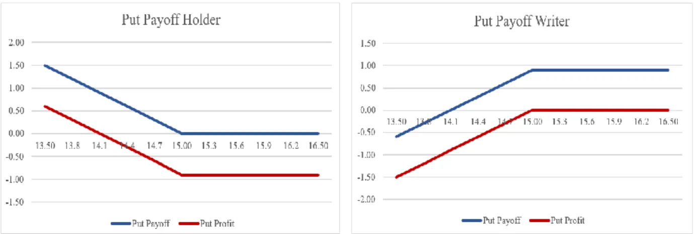
Again, there is two sides: on the one hand, the holder’s profits are limited, exercising the option if the spot price is below the strike price, and not exercising if it is not; on the other hand, the writer earns the premium or has limited losses. The aforementioned can be seen graphically on the Figure 1 and 2.1
Figure 1 Call Options’ payoffs and profits
1 Figures from 1 to 6 were designed by the writer using random numbers, chosen accordingly, on excel.
-2,00 -1,50 -1,00 -0,50 0,00 0,50 1,00 1,50
Call Payoff Writer
Call Payoff Call Profit -1,50 -1,00 -0,50 0,00 0,50 1,00 1,50 2,00
Call Payoff Holder
6
Figure 2 Put Options’ payoffs and profits
Concluding this part, ceteris paribus, the time to maturity is directly proportional to the value of the option, due to the fact that even if the option is out-the-money the spot price can change along the time, therefore the longer the time the bigger the chance to get in-the-money.
2.3. Option Pricing
The most common used method to price an option is the one proposed by Black and Scholes (1973), having certain assumptions:
• The option is European;
• During the life of the option no dividends are paid out;
• Markets are efficient, so market movements cannot be predicted;
• There are not imperfections on the market, so no taxes, short‐selling bans, transactions costs;
• The underlying asset follows a geometric Brownian motion and trading is continuous, knowing that investors have access to unlimited borrowing and lending opportunities;
• The risk-free rate and volatility of the underlying are known and constant; • The returns on the underlying are normally distributed.
Being so, the fair price of a European call option written on an underlying equity would be: 𝐶𝐵𝑆(𝑆, 𝜏, 𝑋, 𝑟, 𝑞, 𝜎) = 𝑆𝑒−𝑞𝜏𝑁(𝑑 1) − 𝑋𝑒−𝑟𝜏𝑁(𝑑2) , (3) -1,50 -1,00 -0,50 0,00 0,50 1,00 1,50 2,00
Put Payoff Holder
Put Payoff Put Profit
-2,00 -1,50 -1,00 -0,50 0,00 0,50 1,00 1,50
Put Payoff Writer
7 where 𝑑1 = log (𝑋) +𝑆 (𝑟 − 𝑞 −𝜎22) 𝜏 𝜎√ 𝜏 , (4) and 𝑑2 = 𝑑1− 𝜎√ 𝜏, (5)
knowing that 𝑁(𝑑1) and 𝑁(𝑑2) correspond to the cumulative probability from the
standard normal distribution of 𝑑1 and 𝑑2, respectively. The parameters still not specified so far are: the risk-free interest rate (r), the dividend yield (q) and the volatility of the underlying asset (𝜎).
In order to derive the above-mentioned, Black and Scholes (1973) based on pricing the option using combinations of the underlying security and a risk-free bond to mimic an option’s payoff structure, Cochrane (2005) solved the appropriate stochastic discount factor and Baz and Chacko (2009) with a probabilistic approach, using the assumption that the price of a security on the present is simply the expected value of it in the future discounted by the risk-free interest rate.
An important concept that will enable us to simplify our calculations is the Put-Call parity. This relates the prices of call and put options, allowing the possibility to explore the existing or nonexisting arbitrage if the two are not connected, this means the possibility of making a profit from holding a call and writing a put or the other way around. It is:
𝑃𝐵𝑆−𝐶𝐵𝑆 = 𝑋𝑒−𝑟𝑡−𝑆𝑒−𝑞𝑡 (6)
which implies,
𝑃𝐵𝑆(𝑆, 𝜏, 𝑋, 𝑟, 𝑞, 𝜎) = 𝑋𝑒−𝑟𝜏𝑁(−𝑑
2) − 𝑆𝑒−𝑞𝜏𝑁(−𝑑1). (7)
Once the risk preferences of agents do not enter the pricing equations, the Black-Scholes pricing formulae will assume risk neutral probabilities. This means the subjectivity of the probability will be replaced, but can have a deceptive conclusion, as the risk neutral probabilities place higher event-probabilities on states with higher utility or disutility. For instance, Cochrane (2005) uses the example that people whom state plane crashes have a high probability, are not irrational, but instead they are reporting
8
their risk neutral probabilities, it means that dying on an airplane crash has a high disutility for the individual.
2.3.1. Pricing currency options
In order to price options, using the Black-Scholes pricing formulae, whose underlying is a foreign currency and the payoff is the foreign interest rate, thus this is what will be included on the formulae, taking out the dividends that are the payoff of the underlying asset, equity or equity index. Thus, as proposed by Garman Kohlhagen (1983) the equation for the fair price of a European call option written on foreign interest rate (𝑟∗) is: 𝐶𝐵𝑆(𝑆, 𝜏, 𝑋, 𝑟, 𝑟∗, 𝜎) = 𝑆𝑒−𝑟 ∗𝜏 𝑁(𝑑1) − 𝑋𝑒−𝑟𝜏𝑁(𝑑2),2 (8) where 𝑑1 = log (𝑋) +𝑆 (𝑟 − 𝑟∗−𝜎22) 𝜏 𝜎√ 𝜏 . (9)
So, as it can be perceived the usage of the dividend yield (q) falls and now it is used the foreign interest rate (r*).
A further simplification to the pricing formula above was proposed by Malz (1997), inserting the forward rate (𝐹𝑡,𝑇):
𝐶𝐵𝑆(𝑄, 𝜏, 𝑟∗, 𝜎) = 𝑁 (−log(𝑄𝑡) − 𝜏 ( 𝜎2 2) 𝜎√𝜏 ) − 𝑄𝑡𝑁 ( log(𝑄𝑡) + 𝜏 (𝜎22) 𝜎√𝜏 ) , (10) in which 𝑄𝑡 = 𝑋𝑡 𝐹𝑡,𝑇. (11)
And the forward rate here is the spot price capitalized to the future date in question, being the equation in the case of currencies the following:
𝐹𝑡,𝑇 = 𝑆𝑡𝑒(𝑟−𝑟
∗)𝜏
. (12)
9
2.3.2. Volatility smile
Facing now the problem of gathering the data for the six parameters above, there is one of these that delivers a more difficulty to obtain, the volatility, while the others are approximately observable or can be perceived: the spot price, the strike price, the time to maturity, the home interest rate and the foreign interest rate. So, in order to get this value, it shall be observed the market prices for options, i.e. the left hand side of the pricing equation, then finding the value that calculates the price suggested by the pricing formulae and the spot price. Nonetheless, sometimes it is impossible to find a closed form solution, so finding a solution will be done through numerical methods instead.
Now introducing the concept of implied volatility: the value of volatility that connects the market price with the pricing formulae. This is a measure of uncertainty of the underlying price at the expiry date.
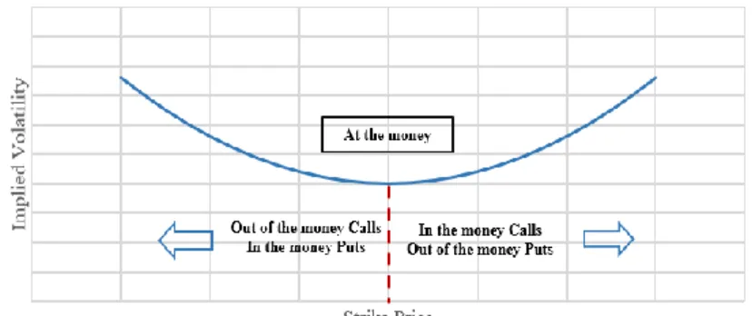
Discovered after the 1987 stock market crash, traders realized that extreme events could happen and markets have a significant skew, thus, in the real world, the implied volatility plots a volatility smile. This one is a graph shape, looking like a smiling mouth, that results from plotting the strike price and implied volatility of a set of options with the same expiry date. Implied volatility rises when the underlying of an option is further in the money or out of the money, compared to the at the money, which is when the volatility tends to be the lowest – see Figure 3.
Figure 3 Volatility Smile
Nevertheless, it must be said that the Black-Scholes model predicts that the implied volatility is flat, when plotted against several strike prices and not curve like in the real
10
world. This happens since the pricing formulae adopts prices changes being log-normally distributed.
In this case, on the currency options, the volatility shows a graph with a smile shape, while on the other hand for options written on equities displays a smirk format, i.e. the implied volatility decreases as the strike price increases – also only noted after the market crash in the 80’s. This can easily be seen by the fact that in the first case the demand for hedging currency options is relatively evenly split between those protecting against appreciation and depreciation, once both groups of economic agents, the ones buying and the ones selling, will have consequences in either cases. While economic agents on the market of equity options are hedging against a fall in equity prices. Thus, demand will not be so regularly distributed between out and in the money options.
Along the time, Hull (2015) says that normally volatility will be mean-reverting. By denoting so, he means that it will be expected to increase if near expiry dates volatilities are low relative to historical experience and be expected to decrease if near term ones are historically high. Adding so that the effect of the smirk or smile turns less and less noticeable as maturity lengthens.
3.OBTAINING RISK NEUTRAL PROBABILITY DENSITY FUNCTIONS
In this third section of the thesis, it will be discussed about the several ways to obtain the Risk Neutral Probability Density (RND) Function and explain two of them. Afterwards there are some concepts that still need to be clarified. And only then, there will be enough material to start applying the model chosen to a real world example and interpret it.
Defining, firstly Risk Neutral Probability is the expectation of possible future payoffs that have been tailored for risk, which as the name says, risk neutral, means that an investor is more concerned on the possible payoff than the risk attached. These probabilities will later be used for figuring fair prices for an asset or financial holding. Not before, though, ensuring a reading of the current situation of the market linked to it, being even able to tag it on the news.
11
The literature regarding the extraction of RNDs Functions is not yet settled, so there is no agreement on whether technique is better than another, as it can be seen by Cooper (1999) and Jondeau and Rocinger (2000) that have compared various methods, nevertheless unable to draw unambiguous conclusions.
One method used is a modified version of Shimko’s (1993) Black Scholes, which consists on fitting the smile with a cubic spline, whose flexibility was improved by Campa, Chang and Reider (1997). However, it has significant drawbacks in terms of implied RND, once in overall it will show kinks, i.e. non-differentiable points corresponding to the knot points of the cubic spline, so the second derivative of a cubic spline is a continuous piecewise linear function. This occurs, not by theory or data, but due to the method of deriving the RND, leading to a difficulty of interpreting as an underlying distribution of the market expectation of the growth in the option’s price.
As seen previously, and as Taylor (2005) denotes, specifying call prices (C(X)) for all possible exercise prices (X) and specifying implied volatilities (σimplied(X)) for the all possible exercise prices are equivalent. After being able to obtain these two, it is possible to specify a risk neutral density (𝐹𝑄(𝑆)) for all possible market prices (S). Nonetheless, these three problems are basically the same and in order to comprehend this, it is needed to collect data from both the call price and the implied volatility through sequential incremental changes on the strike price, which replicates the location and shape of the underlying risk neutral density along the same exercise prices. Summing, in order to have the call prices at all potential strike prices, the implied volatility is also needed at all the potential exercised prices.
On the one hand, the price and its difference between two out of the money call options displays a trend to zero as the strike prices move further out of the money, so that the possibility of it returning to the money tends to zero as so, hence in the long position the market price of the underlying will be below the strike one. Of course, these kinds of options have little likelihood of being exercised, therefore the market does not make much distinction in the price of two long shots. The second difference between prices will also tend to zero.
Whilst, on the other hand the prices of two sequential equally spaced call options deeply in the money will display a trend towards the profit that can be gain from
12
exercising it, and its difference to the incremental difference in price between both options, so that the obvious explanation is the fact that as the price moves further and further in the money, the likelihood of it being exercised increases. In the long position the spot price of the underlying will be above the price agreed upon expiry. If there is a difference in price between the two options, it reflects the difference in profit to be realized on expiry. Here, as before the second difference tends to zero.
Among these two extremes, lies the at or around the money, in which the price of two sequential equally spaced options and the difference in the prices differs at each interval. This happens once the probability reaching a certain level, so that the underlying ends in the money, resulting on being exercised. This characterizes the central part of the distribution. Actually, from stating all possible call prices the mean of the underlying RND can be calculated, there is information regarding the standard deviation of the RND and the distribution’s symmetry (so displaying its skew), and lastly, kurtosis will also be able to be analyzed.
Continuing the reasoning on how to calculate the RND, it will be explained why the Black-Scholes formulae cannot be used. So, firstly in order to have the availability to use this model it is needed the measure of the volatility to specify a call price for every potential strike, therefore using the same information. Hence looking at the aforementioned, laying out the implied volatilities along the strike prices it is being ascertained the volatility smile3. The issue with this model is the fact that once the returns on an asset are log-normally distributed, the implied volatility will be constant for all strike prices, compromising the smile effect on the graph, thus, the RND would also be log-normal.
In the case of equity options, the volatility displays a smirk smile, because implied volatilities decrease as the strike price goes up, giving a downward skew to the distribution. However, in the case of currency options, there is seldom a noticeable smile with implied volatility for at or around the money options lower than for both in and out, so the distribution will likely be symmetric.4
3 The shape and location of the volatility smile depicts the shape and location of the underlying RND,
helping to characterize its skew and kurtosis.
13
Ross (1976) uses a simple and important example of a contingent claim, the Arrow-Debreu (that pays one unit if one sate occurs and zero otherwise), built by a portfolio of European call options. With this synthetic Arrow-Debreu assets is able to establish a relation between option prices and the RND. Cox and Ross (1976), goes even further by ruling out the arbitrage opportunity, therefore demonstrating that options in general, not taking into consideration investors’ risk preferences, can be priced as if investors were risk neutral.
Finally, the method to be used, Breeden and Litzenberger (1978), derived the underlying RND from the volatility smile and call price schedule. Here, it is used the options pricing formulae from Black-Scholes, which ultimately, under risk neutrality, implies that the fair price of a call option is the discounted expectation of the options payoff:
𝐶𝐵𝑆(𝑋𝑇) = 𝑒−𝑟𝑡𝐸𝑄[(𝑆𝑇− 𝑋𝑇)], (13)
which can also be written as
𝐶𝐵𝑆(𝑋𝑇) = 𝑒−𝑟𝑡∫ max (𝑥 − ∞ 0 𝑋𝑇, 0)𝑓𝑄(𝑥)𝑑𝑥 (14) or, 𝐶𝐵𝑆(𝑋𝑇) = 𝑒−𝑟𝑡∫ (𝑥 −∞ 𝑋 𝑋𝑇)𝑓𝑄(𝑥)𝑑𝑥, (15)
where 𝑓𝑄 is the RND. Thus, the fair price of the call price is the weighted sum of all possible outcomes multiplied by their probability of happening. Now, respectively, differentiating one time and two times the call price with respect to the strike price
𝜕𝐶𝐵𝑆(𝑋𝑇) 𝜕𝑋𝑇 = 𝑒−𝑟𝑡∫ 𝑓𝑄(𝑥) ∞ 𝑋 𝑑𝑥 (16) and 𝜕2𝐶𝐵𝑆(𝑋𝑇) 𝜕𝑋𝑇2 = 𝑒 −𝑟𝑡𝑓 𝑄(𝑥), (17) so 𝑓𝑄(𝑥) = 𝑒𝑟𝑡 𝜕2𝐶𝐵𝑆(𝑋𝑇) 𝜕𝑋𝑇2 . (18)
14
Therefore, now we have a function to calculate the RND, through the discounted second derivative of the call price function. Black-Scholes presents an analytical solution (with 𝑑1 and 𝑑2 defined as before) which is,
𝑓𝑄(𝑥) = 𝑁(𝑑2) [ 1 𝜎𝑋𝑇√ 𝜏+ 2𝑑1 𝜎 𝜕𝜎 𝜕𝑋𝑇+ 𝑑1𝑑2𝑋𝑇√ 𝜏 𝜎 ( 𝜕𝜎 𝜕𝑋𝑇) 2 + 𝑋𝑇√ 𝜏𝜕𝑋𝜕2𝜎 𝑇2]. (19)
The result can be applied straightforwardly to the Garman‐Kohlhagen variation.
3.1 Currency options
In foreign exchange (Forex or FX) options tend to be priced not on currency units but in terms of implied volatility. Not only but also, delta (δ) is also an attractive way to price these ones. Delta is the rate of change in value of the option with respect to changes in the spot price and is defined as
δ =𝜕𝐶𝐵𝑆(𝑆𝑇) 𝜕𝑆𝑇 = 𝜕[𝑆𝑒−𝑟∗𝜏𝑁(𝑑1)−𝑋𝑒−𝑟𝜏𝑁(𝑑2)] 𝜕𝑆𝑇 = 𝑒 −𝑟∗𝜏 𝑁(𝑑1), (20)
where 𝑑1 is defined as Garman Kohlhagen wrote. But in order to simplify the formula,
using the modified Garman Kohlhagen formula, Malz (1997) suggests:
δ =𝑒−𝑟∗𝜏(−log(𝑄𝑡)−(
𝜎2 2)𝜏
𝜎√ 𝜏 ). (21)
For a given volatility and strike price delta gives a measure that varies only on the underlying asset price, making available a schedule of changes ready for being analyzed. This means that the exercised prices of in and out of the money options continue with the same distance away from the at the money volatility, even when other components change.
Per Black Scholes assumptions, delta is an estimated measure of the ‘moneyness’ of an option. An at the money option would be stated as 50 delta call or put (so a delta of 0.5), implying that there is a 50% chance that it will expire in the money. Two other important and frequent numbers are 25 delta and 75 delta, meaning, close in the money and out the money calls (or close out and in the money respectively). Nonetheless, it is important to refer that through the put call parity calls and puts with the same strike price
15
have identical implied volatilities, as Malz denotes. Thus, the volatility of an x-delta call equals (1-x)-delta put.
3.1.1 Straddle, Strangle and Risk Reversal
Options tend to be quoted as straddles, strangles and risk reversals and not as simple calls and puts. The way these three are presented on the data acquired from Bloomberg platform will be discussed further ahead.
The first option strategy to be scrutinized here is the straddle, in which the investor holds a position with a call and a put, both at the money, whose strike price and expiration dates are the same. As it can be seen on the Figure 4, the profits of a long straddle are unlimited and there is a limited risk, once the “maximum” loss is the sum of both premiums. Thus, rising or falling of underlying’s price has little importance, as long as it moves, due to the fact that this is a hedge against the volatility. The greater the potential move away from the exercise price the greater the profit. For currency options, the price of a long straddle represents the at the money volatility, so the price of a 50 delta call or put as seen before.
The second option strategy is the strangle that resembles the one above by holding a position on a call and put with the same expiry, notwithstanding it differs by being both (the call and the put) out of the money and having non-matching strike prices. Again, the risk is limited to the sum of both premiums’ two options – Figure 3. Needing a greater level of volatility in the price of the underlying, a strangle is normally cheaper than a straddle as the options are purchased out of the money. For currency options, the price of this strategy is quoted as half of the volatility of X delta call plus a (1-X) delta (or X delta put), minus the volatility of an at the money, 50 delta call. Nonetheless, it is common to see strangles quoted with X=10, 25 and 35.
16
Figure 4 Long Straddle and Long Strangle
A strangle and straddle shorted are neutral strategies and have limited potential profits. As it can be observed on the Figure 5, the maximum profit is equivalent to the net premium received from writing the call and the put.
Figure 5 Short Straddle and Short Strangle
Lastly, the third strategy is called risk reversal, also known as protective collars, investors have the purpose to hedge the position. A long risk reversal writes an out the money put option and purchases an out the money call option, being important an increase on the underlying, unlike the previous strategies that relied only on volatility – Figure 6. On the other hand, a short risk reversal sells a call and buys a put. For currency options, the price of this strategy is quoted as the difference between the volatility of X delta call plus and a (1-X) delta call (or X delta put). Again, these can be quoted as X=10, 25 and 35.
Price
17
Figure 6 Long and Short Risk Reversal
3.1.2 Bloomberg Currency options
The currency options data needed, from 1st of February to 31st of April, can be
extracted from the platform Bloomberg, which can be accessed at ISEG, University of Lisbon. This data, as seen before, will be organized through three contracts that enables the use of the Malz’s approach, the parametric and the non-parametric: strangles, straddles and risk reversals. The nomenclature on this platform although is different. Therefore, the names for strangle, straddle and risk reversal on Bloomberg are, respectively at the money, butterfly and risk reversal and its delta codes V, B and R.
Though, the code is composed by the first six letters being related to the currency pair of the case study, then, normally 10, 25 or 35 delta contract and its form of contract (V, B or R), and lastly the maturity (e.g. 3M for three months). Concluding, a Croatian kuna to a Tunisian dinar, under a 25 butterfly for 1 month is HRKTND25B1M. For the purpose of this thesis, the case will be from a GB (Great Britain) pound to a USA dollar, so in order to implement the parametric approach for three months the codes are: GBPUSDV3M, GBPUSD25B3M, GBPUSD25R3M. For the non-parametric approach additional risk reversals and strangles can be used with 10 and 35 deltas: GBPUSD10B3M and GBPUSD35B3M; GBPUSD10R3M and GBPUSD35R3M.
Apart from these numbers taken to each day between 1st of February and 31st of April, from the same search it can be obtained the spot price and in order for an easier way of collecting all together the days of USD Libor and GBP Libor it is used a different website.5
5“ https://www.global-rates.com/” accessed at first of may of 2019.
18
Notwithstanding the above, it must be said that the 18th of February is the President’s Day holiday in the USA, 19th of April the Good Friday holiday in the USA and GB and, finally the 22nd of April the Easter Monday holiday in GB. Therefore, these days, together with the weekends don’t enter the matrix formulae.
3.2 Parametric implied probability densities from currency options
In this section, in order to calculate the RND, there will be two equations. So, firstly, there will be organized a matrix in excel with date transposed to a five digit number, the spot price, the forward price, the at the money price, the 25 risk reversal price, the 25 butterfly price and finally the USD libor (in this case).
Bahra (1997) calculates the call price function at all potential exercise prices, requiring an estimation for implied volatility at all potential strike prices. It is usual to perform this implied volatility through a functional form, therefore published option prices are merely observations of this function. With this said, firstly, it is needed a function, and as seen before the one to be used for currency options was proposed by Malz (1997):
𝜎(δ)= 𝑏0𝑎𝑡𝑚𝑡+ 𝑏1𝑟𝑟𝑡(δ − 0.5)+ 𝑏2𝑠𝑡𝑟𝑡(δ − 0.5)2. (22)
The at the moment volatility (atm) shows the location of the smile, the risk reversal (rr) shows the skew, and strangle (str) the kurtosis. This approach uses 25 delta risk reversals and strangles. The function, as disposed, is quadratic though the volatility presents a smile shape for currencies. A parametric evaluation assumes the value of a constraint for the purpose of analysis, thus Malz assumes the values for 𝑏𝑖 are:
𝜎𝑎𝑡𝑚 = 𝜎(0.5; 𝜎𝑎𝑡𝑚, 𝑟𝑟, 𝑠𝑡𝑟) = 𝑏0𝜎𝑎𝑡𝑚 (23) 𝑟𝑟 = 𝜎(0.25; 𝜎𝑎𝑡𝑚, 𝑟𝑟, 𝑠𝑡𝑟) − 𝜎(0.75; 𝜎𝑎𝑡𝑚, 𝑟𝑟, 𝑠𝑡𝑟) =𝑏1 2 𝑟𝑟 (24) 𝑠𝑡𝑟 =𝜎(0.25;𝜎𝑎𝑡𝑚,𝑟𝑟,𝑠𝑡𝑟)+𝜎(0.75;𝜎𝑎𝑡𝑚,𝑟𝑟,𝑠𝑡𝑟) 2 − 𝜎𝑎𝑡𝑚 = 𝑏2 16𝑠𝑡𝑟 (25) so that, 𝜎(δ)= 𝑎𝑡𝑚𝑡+ 2𝑟𝑟𝑡(δ − 0.5)+ 16𝑠𝑡𝑟𝑡(δ − 0.5)2. (26)
19
Satisfying the functional form, if the observed volatility is at the money, this means delta = 0.5. So, substituting the deltas in equation 22, the values of the risk reversal and strangle will be zero. Therefore, the coefficient on the at the money volatility must be 1.
Now, with this equation there is two unknown values, delta and volatility, so, as said in the beginning of this sub chapter, there will be needed another formula with this two values, but instead of being volatility in terms of delta it will be delta in terms of volatility. This equation is the 21.
Applying these two equations, 21 and 26, to codes on MATLAB will solve simultaneous equations at each potential strike price, in currency units, providing values for implied volatility and delta at those strike prices.
Concluding, as soon as the values for implied volatilities are determined for each strike price, having sigma, these can be placed into the modified call price function for Foreign Exchange options, determining the price at every potential strike. After this, using the diff function on MATLAB6 the second derivative of the call price function can be ascertained, giving the closer risk neutral probability density.
Figure 7 Scheme for RND on Parametric approach
3.3 Nonparametric implied probability densities from currency options
Before starting to explain this method, and continuing the above structure, it is needed to do an array in excel with a date transposed to a five digit number, the spot price, the at the money price, the 10, 25 and 35 risk reversal prices, the 10, 25 and 35 butterfly prices and finally the USD and GBP libor prices (in this case).
Facing the method above, there is already a more recent style proposed by Malz (2014), not requiring assumptions for the shape of the volatility smile, thence nonparametric. This new method has also another advantage, which is the fact that it can
6 Diff (X,2) is the same as diff(diff(X)).
Gather Information
Delta Sigma
Call Price Second Derivative
RND Graph
20
be implemented almost the same way through different asset classes, such as interest rates, equities and foreign exchange. In order to continue, there is three steps to complete: interpolate and extrapolate the volatility smile with a clamped cubic spline (see Appendix B) with flat ends; make use of the call option price function to give back the interpolated volatilities into currency units options; and, finally, as seen before, use Breeden-Litzenberger result and take the second differences of the call option price function to obtain the density.
Although there are some issues that need to be surpassed, the utilization of this process considering currency options is fairly simple.
For the first step it is necessary to compile the currency options volatilities at different deltas in and out-the-money. It is needed, considering the prices in question, to compute the volatilities at 10, 25, 35, 65, 75 and 90 delta given that for the majority currency pairs, Bloomberg only shows data for strangles and risk reversals at 10, 25 and 35 delta.
The risk reversal and the strangle prices (rr and str) as Malz (1998) depicts them are defined as:
𝑠𝑡𝑟 = 0.5(𝜎75𝛿+ 𝜎25𝛿) − 𝜎𝑎𝑡𝑚, (27)
𝑟𝑟 = 𝜎25𝛿 − 𝜎75𝛿 . (28)
Therefore, the following equations allow the calculation of the volatility delta at the different moneyness levels:
For X = 10, 25 and 35
𝜎𝑋𝛿 = 𝑎𝑡𝑚 + 𝑠𝑡𝑟 + 0.5 𝑟𝑟 (29)
For X = 65, 75 and 90
𝜎𝑋𝛿 = 𝑎𝑡𝑚 + 𝑠𝑡𝑟 − 0.5 𝑟𝑟 (30)
During this stage to overcome the fact that the at-the-money volatility has a delta that is not an exact value but close to it, in this case the value is 50, it is possible to compute this number taking the first formula and setting the strike price equal to the current spot price.
Concluding this step, there are available 7 data points that can be applied to sketch the volatility smile using a clamped cubic spline. From this, it is possible to get a value
21
for volatility at all conceivable deltas. In order to fill the call price function, it is needed the volatilities at all potential exercise prices in currency units. It happens that, as Malz records, it is not conceivable to link volatility to delta space volatility to strike price space through the delta function, once the volatility argument in the equation is not constant, being directly linked to the delta, so fluctuating with it. Nonetheless, to find the closer value to volatility, related to exercise price, it will be needed numerical methods. So, having the implied volatility at each strike price, it is calculated the delta value, which will be the same as the delta value calculated using the cubic spline function. Iterating the aforementioned: 𝜎𝑠+1 = 𝜎𝑠 (31) 𝛿̂ = 𝑒−𝑟∗𝜏𝑁 ((log 𝑆 𝑋)+(𝑟−𝑟 ∗−𝜎𝑠2 2 )𝜏 𝜎𝑠√𝜏 ) (32) 𝜎𝑠+1 = 𝑎𝑘+ 𝑏𝑘(𝛿̂ − 𝛿𝑘) + 𝑐𝑘(𝛿̂ − 𝛿𝑘) 2 + 𝑑𝑘(𝛿̂ − 𝛿𝑘) 3 (33)
So, as seen on the Appendix B, 𝑎𝑘, 𝑏𝑘, 𝑐𝑘 and 𝑑𝑘 are arguments from cubic spline evaluated at 𝛿𝑘 the observed volatilities, constructing the knot points to interpolate.
Therefore, it is being chosen the right value of implied delta (𝛿̂) to calculate the values of the implied volatility (𝜎). After doing so, with delta and sigma calculated, the call option price can be ascertained at the strike price.
The next step is to repeat the process through the several strike prices so that the density can be drawn. Thus, the right values of the knot points must move between the noted values of the implied volatility. Doing so, the sigma is calculated for all potential exercise prices, making it available to calculate the call prices and then perform the numerical second difference, determining the closer risk neutral probability density.
22
Figure 8 Scheme for RND on Nonparametric approach
3.4 Application
Now that it is expressed here the method to calculate the RND with a parametric and a nonparametric approach, it is time to apply to a real case and read it. So, as said before it will be used MATLAB coding. They are on Appendix A, the coding regarding the parametric approach, and on Appendix B the explanation of the natural and clamped splines to be used on the Appendix C, where the programming codes for the nonparametric method can be seen.
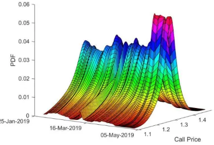
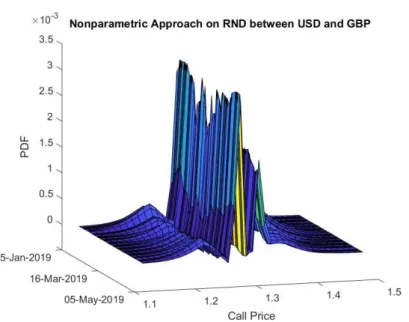
The example used to test the methods is between the USA dollar and the GB pound, between February and April of 2019, organising on a single sheet the date, the forward rate, the spot price, the at the money price, the 10, 25 and 35 risk reversal prices, the 10, 25 and 35 butterfly prices and finally the USD and GBP libor prices. As said in the introduction these two currencies were chosen due to big news they had during this last year of 2019. Subsequently, after computing the result is Figure 9 for the RND through a Parametric approach and Figure 10 for a Nonparametric approach.
Gather Information
Set up Volatility Smile Observed Points Call Price Second Difference RND Graph Cubic Spline
23
Figure 9 Parametric Approach on RND between USD and GBP
Looking at Figure 9 and 10, the first thing that pops out is the fact that the location of the density does not change much and the fact that the parametric method presents a more regular surface compared to the nonparametric one. This happens due to the fact that on the first approach the shape of the volatility smile is being imposed, certifying that all stated volatilities are hit by the assumed volatility function. Nonetheless, the nonparametric style is more accurate, but is susceptible to more imperfections while market pricing on illiquid contracts, influencing the shape of the volatility smile.
It is interesting to note on Figure 9 that close to the middle of march the density does not appear so peaked, which means that there was a period of big uncertainty; and there seems a greater peak on the left hand size of the tail, meaning that investors were insuring against the depreciation on the GB pound, thus USA dollar appreciation. Relating this variance to the news, it is observed that the agreement for United Kingdom (UK) to leave the European Union (Brexit) that was due to 29th march of 2019 had to be delayed to 12th April of 2019, however the negotiations internals in UK and between them and the European Union were not being successful, therefore there appeared another extension to 31st October of 2019. This bigger extension may be behind the reason why the end of march presents a more peaked density, which means a higher certainty. On the other hand,
24
there is the USA that even with the trade war with China (that affects all countries) presents a robust economy.
Figure 10 Nonparametric Approach on RND between USD and GBP
In the end, it is important to refer the error estimation related to these two models. While doing the parametric approach on RND it can be perceived that it uses less information than the nonparametric approach, so the error is linked to the fact that lacks data and assumes some other values as fixed. On the other hand, the nonparametric approach uses to much values that float at the same time, plotting a curve not as smooth as the one from the first approach, making it harder to read also.
25
Risk Neutral Probability Density for currency options and none of them is perfect. With this thesis it was intended to show the best two recent methods from a wide range of models available (in the opinion of the writer). Nonetheless, as it can be seen the nonparametric method used presents some irregularities linked to precisely the fact that the volatility smile is not imposed. A future guideline can be said that depending on the information gathered it can be more advantageous to use a parametric rather than a more accurate nonparametric method.
It was possible, to construct two graphs, being easy to link its reading to the news, which is a good sign, specially from the first one.
The computation of the RND is not done only for the purpose of reading on the period that it is related, but to predict the evolution of the underlying. In the case used for study, in the overall, there appears to be a slight appreciation of the USA dollar compared to the GB pound, which was a good foresee, but mostly because in the beginning of June the Prime Minister of UK, Theresa May, resigned, being elected a new one through internal party elections on late July, Boris Johnson. It happens that in August the pound reached the lowest in two years. This linked to the fact that USA’ Gross Domestic Product is growing more than the prediction.
Finalising, for further investigation there could be constructed a program or simply link the information automatically from a data base like Bloomberg or another, allowing the researcher to make predictions up to date, for the different methods, so in the end he the researcher would use the best model accordingly.
26
Densities by Fitting Implied Volatility Smiles: Some Methodological Points and an Application to the 3M Euribor Futures Option Prices, European Central Bank,
Working Paper No. 198
Baz, J. and Chacko, G. (2009). Financial Derivatives: Pricing, Applications and
Mathematics, Cambridge University Press
Black, F. and Scholes, M. (1973). The pricing of options and corporate liabilities, Journal of Political Economy 81:637‐659
Blake, Andrew and Rule, Garreth (2015). Deriving option-implied probability densities
for foreign exchange markets, Bank of England.
Breeden, D.T. and Litzenberger, R.H. (1978). Prices of state‐contingent claims implicit
in options prices, Journal of Business 20:419‐438
Bahra, B. (1997). Implied risk‐neutral probability density functions from options prices:
Theory and application, Bank of England Working Paper No. 66
Brandao, Mark (2014). Natural and Clamped Cubic Splines, Math 4446 Project I
Campa, José M., Chang, P. H. Kevin and Reider, Robert L. (1997). Implied Exchange
rate Distributions: Evidence from OTC Option Markets, NBER Working Paper
no. 6179
Cochrane, J.H. (2005) Asset Pricing, Princeton University Press, revised edition
Cooper, Neil (1999). Testing Techniques for estimating Implied RNDs from the prices of
European-style Options, Bank of England Working Paper
Cox, John and Stephen, Ross (1976). The Valuation of options for Alter-native Stochastic
27
Garman, M.B. and Kohlagen, S.W. (1983). Foreign currency option values, Journal of International Money and Finance 2:231‐237
Hull, J. C. (2015). Options, Futures and Other Derivatives, Pearson, ninth edition Jondeau, Eric and Rockinger, Michael (2000). Reading the Smile: The Message Conveyed
by Methods which Infer Risk Neutral Densities, Journal of International Money
and Finance 19: 885-915
Klugman, S. A., Panjer, H. H., and Willmot, G. (2008). Loss Models: From Data to
Decisions. Wiley, New York, third edition.
Malz, A. M. (1997). Option‐implied probability distributions and currency excess
returns, FRBNY Staff Reports No. 32
Malz, A. M. (1998). Interbank interest rates as term structure indicators, Federal Reserve Bank of New York, Research Paper 9803
Malz, A. M. (2014). A Simple and Reliable Way to Compute Option‐Based Risk‐neutral
Distributions, FRBNY Staff Reports No. 677
Mandler, Martin (2003). Market Expectations and Option Prices, Springer-Verlag Berlin Heidelberg GmbH.
Ross, Stephen (1976). Options and Efficiency, Quarterly journal of Economics 90: 75-89 Shimko, David (1993). Bounds of probability, RISK 6: 33-37
Taylor, S. J. (2005). Asset Price Dynamics, Volatility and Prediction, Princeton University Press
28
Firstly, on a separate sheet it is created the function of the delta volatility that has to be saved.
function [delta, sigma] = functvoldel(delta, sigma, atm, rr, bf, rstar, t, q) 1 Vold = delta+sigma+1; 2 while abs(delta+sigma-Vold)>0.0000001 3 Vold = delta+sigma; 4 sigma = atm-2*rr*(delta-0.5)+16*bf*(delta-0.5)^2; 5 d = -(log(q)-sigma*sigma*t/2)/(sigma*sqrt(t)); 6 delta = exp(-rstar*t)*0.5*erfc(-d/sqrt(2)); 7 end 8 end 9
Then, on a different sheet, it starts by opening the excel with the information needed, succeeding with its right manipulation. Then it is set the storage matrixes for the loop that comes after, solving the sigma and delta equations, so that there are arguments for the call price function. Still inside the loop the probability density function is calculated with the second derivative of the call. In the end this is all plotted resulting on the pretended graph.
cd('C:\Users\FranciscoLopes\Google Drive\Finance\Thesis'); 1
data = xlsread('Excel_Thesis.xlsx','MATLABParametric','B3:H62'); 2 3 datesMATLAB = (x2mdate(data(:,1))); 4 dates = datestr(datesMATLAB); 5 spot = timeseries(data(:,2),dates); 6 FWD = timeseries(data(:,3),dates); 7 ATM = timeseries(data(:,4),dates); 8 RR25 = timeseries(data(:,5),dates); 9 BF25 = timeseries(data(:,6),dates); 10 usdlibor = timeseries(data(:,7),dates); 11 12 rstar = usdlibor.Data/100; 13 fwd = FWD.Data; 14 atm = ATM.Data/100; 15 rr = RR25.Data/100; 16 bf = BF25.Data/100; 17 t = 3/12; 18
29 19 xax = (1.1:0.005:1.5)'; 20 xaxis = xax(3:end); 21 22 pdf = nan(length(xax)-2,length(dates)); 23 24 for j = 1:length(dates)-1 25 q = xax/fwd(j); 26 delta = nan(length(xax),1); 27 sigma = nan(length(xax),1); 28 for k=1:length(xax) 29
[delta(k), sigma(k)] = functvoldel(0.5,1,atm(j),rr(j),bf(j),rstar(j),t,q(k)); 30 end 31 d1 = -(log(q)-sigma.^2*t/2)./(sigma*sqrt(t)); 32 call = 0.5*(erfc(-d1/sqrt(2))-q.*erfc(-(d1-sigma*sqrt(t))/sqrt(2))); 33 pr = diff(call,2); 34 pdf(:,j) = pr/sum(pr); 35 end 36 37 figure 38 surface(datesMATLAB,xaxis,pdf) 39
title('Parametric Approach on RND between USD and GBP') 40
ylabel('Call Price') 41 zlabel('PDF') 42 dateaxis('x',1) 43 colormap hsv 44 view([90-55,12]) 45
APPENDIX B NATURAL AND CLAMPED SPLINES
One of the steps required to calculate the nonparametric RND from currency options using cubic spline is to interpolate and extrapolate the volatility smile. In order to complete this mission, Malz used a variation on the standard cubic spline, branded as a clamped spline. So, basically, a standard cubic spline is simply the set of a sequence of cubic functions defined through the intervals between the observed points, whose functions are subject to a couple of restraints that guarantee their behaviour on the interpolating interval. Nonetheless, the clamped spline behaves in a way that with specific assumptions the first and last knot points make the curve become constant at chosen values. A more thorough explanation of the derivation of cubic spline coefficients can be found in Klugman et al. (2008).
30
The first of five cubic splines characteristics is the definition of the cubic function piecewise between the observed data points (equation B.1).
𝑦̂𝑗 = 𝑎𝑗+ 𝑏𝑗(𝑥 − 𝑥𝑗) + 𝑐𝑗(𝑥 − 𝑥𝑗)2+ 𝑑𝑗(𝑥 − 𝑥𝑗)3 = 𝑓𝑗(𝑥) 𝑓𝑜𝑟 𝑥𝑗 ≤ 𝑥 ≤ 𝑥𝑗+1 (B. 1)
The second cubic spline property is to pass through all the data points, so it maintains at the observed data point the interpolated value as the same (equation B.2).
𝑦̂𝑗 = 𝑓𝑗(𝑥𝑗) = 𝑦𝑗 (B. 2)
The third, in order to maintain the interpolated line continuous, the value at the end of a period is identical to the beginning of the next one (equation B.3).
𝑓𝑗(𝑥𝑗+1) = 𝑓𝑗+1(𝑥𝑗+1) (B. 3)
The fourth and fifth characteristics have the core to keep a smooth curve, maintaining the continuity of the first and second derivatives on the points where the functions meet (equations B.4 and B.5).
𝑓𝑗′(𝑥𝑗+1) = 𝑓𝑗+1′ (𝑥𝑗+1) (B. 4)
𝑓𝑗′′(𝑥𝑗+1) = 𝑓𝑗+1′′ (𝑥𝑗+1) (B. 5)
This cubic spline function is a polynomial function, thus it needs arguments. Consequently, to deliver the necessary spline it is needed to gauge esteems for a, b, c and d over the n interims between watched n+1 information focuses, so altogether 4n coefficients are required. Property two gives n+1 conditions that must hold (the quantity of information focuses) while properties 3–5 each give n‐1 conditions (the quantity of interims short one since they are conditions that hold at the two parts of the bargains). Thus, we have n+1+3(n‐1) = 4n‐2 conditions for the 4n coefficients required. Two extra conditions are required to remarkably decide the estimations of the coefficients: ordinarily these two conditions are utilized to decide the shape at the end‐point of the addition. Decision of the end‐points offers ascend to various sorts of spline, which we examine underneath.
On the off chance that 𝑚𝑗= 𝑓𝑗''(𝑥𝑗) and the number the perceptions from 0 to n, it can
written in matrix structure:
31 where, 𝐻 = [ 2(Δ𝑥1+ Δ𝑥2) Δ𝑥2 0 0 Δ𝑥2 2(Δ𝑥1+ Δ𝑥3) ⋯ ⋮ 0 0 ⋮ ⋮ ⋱ Δ𝑥𝑛−1 0 0 Δ𝑥2 2(Δ𝑥𝑛−1+ Δ𝑥𝑛)] (B. 7) 𝑢 = [ 6 (Δ𝑦2 Δ𝑥2− Δ𝑦1 Δ𝑥1) − Δ𝑥1𝑚𝑛 6 (Δ𝑦3 Δ𝑥3− Δ𝑦2 Δ𝑥2) ⋮ 6 (Δ𝑦𝑛 Δ𝑥𝑛 − Δ𝑦𝑛−1 Δ𝑥𝑛−1) − Δ𝑥1𝑚𝑛] (B. 8) 𝑚 = [ 𝑚1 ⋮ 𝑚𝑛−1 ] (B. 9)
On the other hand, if it is made a few suppositions with respect to the estimations of 𝑚0 and 𝑚𝑛, it is known that the majority of the qualities in H and u can be computed for
m from:
𝑚 = 𝐻−1𝑢 (B. 10)
Then, it is possible to solve a, b, c and d through the subsequent: 𝑎𝑖 = 𝑦𝑖 (B. 11) 𝑏𝑖 =Δ𝑦𝑖 Δ𝑥𝑖 − Δ𝑥𝑖 6 (2𝑚𝑖−1+ 𝑚𝑖) (B. 12) 𝑐𝑖 =𝑚𝑖 2 (B. 13) 𝑑𝑖 = 𝑚𝑖− 𝑚𝑖−1 6Δ𝑥𝑖 (B. 14)
The most widely recognized type of spline is the supposed normal spline, where the second derivatives at the end focuses are set to zero, henceforth 𝑚0 = 𝑚𝑛 = 0. For the
32
clamped spline- Brandao (2014) explains through examples really well the difference between natural and clamped splines using MATLAB codes - it is rather fixed the first derivative of the end focuses to some fixed worth (for this situation it is zero with the goal that the incline of the bend is level toward the end focuses, however it could be anything). By setting 𝑓′𝑗(𝑥𝑗) = 𝑓′𝑗+1 (𝑥𝑗+1) = 0 this infers:
𝑚0 = 3 Δ𝑦1 ∆𝑥12− 𝑚1 2 (B. 15) 𝑚0 = −3 Δ𝑦𝑛 ∆𝑥𝑛2 −𝑚𝑛−1 2 (B. 16) Now, making some changes to H and u:
𝐻 = [ 1.5Δ𝑥1+ 2Δ𝑥2 Δ𝑥2 0 0 Δ𝑥2 2(Δ𝑥1+ Δ𝑥3) ⋯ ⋮ 0 0 ⋮ ⋮ ⋱ Δ𝑥𝑛−1 0 0 Δ𝑥2 2Δ𝑥𝑛−1+ 1.5Δ𝑥𝑛)] (B. 17) 𝑢 = [ 6 (Δ𝑦2 Δ𝑥2− Δ𝑦1 Δ𝑥1) − 3 ∆𝑦1 ∆𝑥1 6 (Δ𝑦3 Δ𝑥3− Δ𝑦2 Δ𝑥2) ⋮ 6 (Δ𝑦𝑛 Δ𝑥𝑛− Δ𝑦𝑛−1 Δ𝑥𝑛−1) + 3 ∆𝑦𝑛 ∆𝑥𝑛] (B. 18)
Now the above will be applied on MATLAB coding to be used afterwards on the calculation of the RND through the nonparametric method. So, in two different sheets two functions will be defined.
So firstly, the cubic_spline.
function [a, b, c, d] = cubic_spline(x,y,nc) 1
% set nc = 0 for clamped
2
% = anything else for natural
3 4
% Define differences
33 dy = y(2:end)-y(1:end-1); 6 h = x(2:end)-x(1:end-1); 7 8
% Cubic spline: Natural and clamped use H and u
9 H = diag(2*(h(1:end-1)+h(2:end)))+diag(h(2:end-1),1)+diag(h(2:end-1),-1); 10 r = 6./h; 11 z = zeros(length(r)-1,1); 12
R = [diag(r(1:end-1)) z z] + [z -diag(r(1:end-1)+r(2:end)) z] + [z z diag(r(2:end))]; 13
u = R*y; 14
15
if nc == 0 % Clamped flat (zero 1st deriv at boundary)
16
H(1,1) = 1.5*h(1) + 2*h(2); 17
H(end,end) = 1.5*h(end) + 2*h(end-1); 18
u(1) = u(1) - 3*dy(1)/h(1); 19
u(end) = u(end) + 3*dy(end)/h(end); 20 mc = H\u; 21 m = [3*dy(1)/(h(1)^2)-mc(1)/2; 22 mc; 23 -3*dy(end)/(h(end)^2)-mc(end)/2]; 24
else% Natural spline (zero 2nd deriv at boundary)
25 m = [0; H\u; 0]; 26 end 27 28
% Making easier calculation shift m by 1.
29 me = m(2:end); 30 m1 = m(1:end-1); 31 32 % Calculate coefficients 33 a = y(1:end-1); 34 b = dy./h - h.*(2*m1 + me)/6; 35 c = m1/2; 36 d = (me-m1)./(6*h); 37 end 38
And then the cubic_spline_v.
function f_interp = cubic_spline_v(xaxis,a,b,c,d,x,y) 1 j = 0; 2 f_interp = zeros(max(size(xaxis)),1); 3 for xi = xaxis 4 j = j+1; 5 seg = sum(xi>=x); 6 if seg > length(a) 7 if c(1) == 0 8 seg = length(a); 9 else 10 f_interp(j) = y(end); 11
34 continue 12 end 13 elseif seg < 1 14 if c(1) == 0 % 2nd deriv at start = 0 15 seg = 1; 16 else 17 f_interp(j) = y(1); 18 continue 19 end 20 end 21
f_interp(j) = a(seg) + b(seg)*(xi-x(seg)) + c(seg)*(xi-x(seg))^2 + d(seg)*(xi-x(seg))^3; 22
end
23
end
24
APPENDIX C NONPARAMETRIC APPROACH ON RND BETWEEN USD AND
GBP
Again, it will, firstly, on two new sheets will be constructed two different functions. Where, the first is the Black-Scholes formula for Delta function.
function delta = functdelta(S,t,X,r,q,sigma) 1 v = (log(S./X)+t*(r-q+0.5*sigma.^2))./(sigma*sqrt(t)); 2 delta = 0.5*exp(-q*t).*erfc(-v/sqrt(2)); 3 end 4
Then, the Call Option Price on the Black Scholes perspective:
function c = call_bs(s,t,x,r,q,v) 1 vt = v*sqrt(t); 2 d1 = (log(s./x)+t*((r-q)*0.5*v.^2))./vt; 3 c = 0.5*s*exp(-q*t).*erfc(-d1./sqrt(2)) - 0.5*x*exp(-r*t).*erfc(-(d1-vt)./sqrt(2)); 4 end 5
Now, there is enough functions defined in order to start the plotting of the pretended RND. Hence, it is opened a new sheet that starts with extracting the excel information and its manipulation. Then it is set the storage matrix for the loop to come. So, the loop starts by setting up the volatility smile observed points, followed by the computation of the natural cubic spline and the call price with the help of the cubic_spline_v function to define the implied volatility. In the end of the loop the second difference is made with the
35
call option, resulting on the probability density function. The only remaining thing is to plot the surface pretended resulting on the RND for the nonparametric approach.
cd('C:\Users\FranciscoLopes\Google Drive\Finance\Thesis'); 1
data = xlsread('Excel_Thesis.xlsx','MATLABNon-Parametric','B3:L62'); 2 3 datesMATLAB = (x2mdate(data(:,1))); 4 dates = datestr(datesMATLAB); 5 SPOT = timeseries(data(:,2),dates); 6 ATM = timeseries(data(:,3),dates); 7 RR10 = timeseries(data(:,4),dates); 8 RR25 = timeseries(data(:,5),dates); 9 RR35 = timeseries(data(:,6),dates); 10 BF10 = timeseries(data(:,7),dates); 11 BF25 = timeseries(data(:,8),dates); 12 BF35 = timeseries(data(:,9),dates); 13 usdlibor = timeseries(data(:,10),dates); 14 gbplibor = timeseries(data(:,11),dates); 15 16
iv10 = (ATM.Data + BF10.Data + RR10.Data/2)/100; 17
iv90 = (ATM.Data + BF10.Data - RR10.Data/2)/100; 18
iv25 = (ATM.Data + BF25.Data + RR25.Data/2)/100; 19
iv75 = (ATM.Data + BF25.Data - RR25.Data/2)/100; 20
iv35 = (ATM.Data + BF35.Data + RR35.Data/2)/100; 21
iv65 = (ATM.Data + BF35.Data - RR35.Data/2)/100; 22 23 atm = ATM.Data/100; 24 r = gbplibor.Data/100; 25 q = usdlibor.Data/100; 26 S = SPOT.Data; 27 28 xax = 1.1:0.01:1.5; 29 t = 3/12; 30 all_pdf = []; 31 32 for j = 1:length(atm) 33
iv = [iv10(j) iv25(j) iv35(j) atm(j) iv65(j) iv75(j) iv90(j)]'; 34 atmv = functdelta(S(j),t,S(j),r(j),q(j),atm(j)); 35 delta = [.10 .25 .35 atmv .65 .75 .90]'; 36 37 [a, b, c, d] = cubic_spline(delta,iv,0); 38 sv = 0*xax'; 39 iv_n = sv + atm(j); 40 delta_n = functdelta(S(j),t,xax',r(j),q(j),iv_n); 41 42 43
36
while max(abs(sv-iv_n)) > 1e-10 44 sv = iv_n; 45 iv_n = cubic_spline_v(delta_n',a,b,c,d,delta,iv); 46 delta_n = functdelta(S(j),t,xax',r(j),q(j),iv_n); 47 end 48 call = c_bs(S(j),t,xax',r(j),q(j),iv_n); 49 50 df = (call(2:end)-call(1:end-1)); 51 pdf = (df(2:end)-df(1:end-1)); 52 all_pdf = [all_pdf pdf]; 53 end 54 55 figure 56 surface(datesMATLAB,xax(3:end-2),all_pdf(3:end,:)) 57
title('Nonparametric Approach on RND between USD and GBP')
58
ylabel('Call Price') 59 zlabel('PDF') 60 dateaxis('x',1) 61 colormap parula 62 view([90-16.5,12]) 63