UNIVERSIDADE CATÓLICA
PORTUGUESA
PORTO
FACULDADE DE ECONOMIA E GESTÃO
Masters in Finance
Improving Pairs Trading
Tiago Roquette S. C. Almeida October 2011
2 Improving Pairs Trading
Tiago Roquette Almeida Supervisor: Professor Paulo Alves
Universidade Católica Portuguesa - Centro Regional do Porto Faculdade de Economia e Gestão
October 2011
Abstract
This paper tests the Pairs Trading strategy as proposed by Gatev, Goetzmann and Rouwenhorts (2006). It investigates if the profitability of pairs opening after an above average volume day in one of the assets are distinct in returns characteristics and if the introduction of a limit on the days the pair is open can improve the strategy returns. Results suggest that indeed pairs opening after a single sided shock are less profitable and that a limitation on the numbers of days a pair is open can significantly improve the profitability by as much as 30 basis points per month.
3 Who risks nothing risks losing it all
Tiago Almeida
I would like to acknowledge all that believed I would do it:
Professor Paulo Alves, Joana, Pedro, my family, friends and co-workers. You were right but reckless.
4
Index
I. Introduction……… 5
II. Pairs Trading Review……….. 7
2.1. The Strategy……… 7
2.2. Unresolved Questions……….. 12
2.3. Keeping the Rationale, Improving Performance……….……… 14
2.3.1. Opening Pairs after Shocks……… 14
2.3.2. Applying a Limit to the time a Pair is Open………. 15
III. Data and Methodology……… 17
3.1. Sample……….. 17
3.2. Pairs Formation and Trading Period………..……… 18
3.3. Returns……….……… 21
3.4. Variations……….………… 21
IV. Results.……… 24
4.1. GGR Results after 2002……….……… 24
4.2. Limiting the Time a Pair is Open……….. 26
4.3. Volume Events……….. 28
5
I. Introduction
The general principle of the efficient markets hypothesis in the strong form1 (Fama
1970) states that in an informational efficient market “security prices at any time fully reflect all available information” (Fama 1970, 383). This principle implies that returns should be the product of risk taking and excess risk adjusted returns should only be attained by luck so getting them in a systematic way is a violation of this principle.
This academic hypothesis is in an everyday challenge in the marketplace. Many participants believe in their ability to outperform the market and achieve better risk adjusted returns. The existence of portfolio managers that report outstanding cost adjusted returns for extended periods of time raises doubts into the extent markets are efficient.
To address these questions several empirical market tests have been conducted through the years that attempt to investigate to which extent are financial markets in fact efficient (testing the three forms of efficiency). And it takes just one exception to prove that a market is inefficient (as opposed to proving that is efficient, which requires that all possible strategies are proven efficient) but that alone is not an easy task. It’s not simple to measure risk and cost adjusted returns.
Excess returns can remain unexplained because of unidentified risks factors like extreme events (event risk) that are yet to happen. Liquidity, political and
1
Fama 1970 defines three forms of efficiency: the weak form, that states that prices reflect all publicly available information, the semi-strong form, that states that prices reflect all publicly available information and instantly adjust to reflect new publicly available information and the strong form that states that prices reflect relevant monopolistic information.
6 regulatory risk can be difficult to quantify. For example, the risk that regulators prohibit short selling2 has to be accounted for in strategies that short securities.
Operational risk is always present and is naturally higher when strategies have to be implemented via electronic execution with computer programming. The cost to raise capital or the cost of information gathering can also help to explain excess returns in strategies that need these structures. Transactions costs are sometimes difficult to quantify and can dramatically reduce the profitability of these strategies. Therefore when testing for market efficiency, is imperative that a simple strategy is used to explore a possible anomaly, one that can be simply evaluated in terms of risks and costs involved and one that could be easily implemented by market participants.
One simple test (of the weak form of efficiency) can be conducted by evaluating the profitability of a pairs trading strategy that is build only with historical price and volume data.
2
There are several situations when regulators prohibited short selling. For example, the U.S. Securities and Exchange Commission prohibited short selling from 19 September 2008 to 2 October of 2008 because of the increased volatility of price assets.
7
II. Pairs Trading Review
2.1. The Strategy
The pairs trading strategy has a simple rationale: If one cannot price a red apple, one can at least say that two perfectly good red apples (equal in all characteristics) in the same place in time and space are worth the same (assuming rationality). And we can go further, we can assume that there is some stable relationship between the price of a red apple and a green one in the stated conditions.
Pairs trading is an investment strategy that is based on this relative value rationale. First introduced academically by Gatev, Goetzmann and Rouwenhorts (2006) (hereafter “GGR”) pairs trading looks for violations of the law of one price and explores the principle that if two financial assets (most commonly stocks) have the same value and risk drivers, then their relative price should be a stable relationship. This means that their systematic risk is approximately the same and if this relation remains stable in time (if there are no idiosyncratic shocks on either asset) then a long short position should produce a risk free (beta neutral) portfolio with an excess return (over a risk free benchmark asset) of zero.
On the contrary, if the value and risk drivers remain the same but the price relationship doesn’t, then the relative miss price can be explored when is large enough to cover the risks and costs involved. In such cases it is expected that this spread will revert to the historical values when markets participants acknowledge the discrepancy so the strategy would buy the asset with the relative price
8 decrease, sell the one with the relative price increase and wait for a convergence in the relative price to close the position.
There are several ways in which the pairs trading strategy can be implemented. In the work of GGR pairs of similar assets (listed stocks on US equity market) are discovered through a period of pairs formation (a training period) consisting of 250 working days (the equivalent to a trading year). In this period pairs are formed with all available assets in the sample, this is, if a sample of 5 stocks is used then 10 possible pairs can be formed as is showed in the following example:
5!
2! 5 2 ! 10
With all possible pairs formed we then evaluate how similar those pairs are using only the daily price data. For that purpose GGR proposes a closeness measure that first normalizes the prices of the assets that form a pair to the first day of the 250 days training period and then sums the absolute daily spread for that period. If the prices of the two assets in the pair are a linear combination for the whole 250 days period then the closeness measure would be 0. This measure is proposed as proxy of how similar the assets are.
With this measure calculated for all the possible pairs that have price data in the period the top 20 pairs, which are the ones who have the smallest closeness value, are taken into a trading period of 125 working days (equivalent to half a trading year). In this period the chosen pairs are monitored and if the spread between the assets of a top 20 pair becomes wider than 2 historical standard deviations (calculated in the training period) a Long/Short position is taken. When and if prices
9 cross (the spread between the normalized prices crosses 0) again the position is unwind. If at the end of the trading period a position is opened or if one of the stocks in the pair is delisted then the position is unwind.
Chart 1 is an example of a 250 trading days period for a pair of very similar assets and Chart 2 is a representation of the following 125 trading days period.
Chart 1
The chart shows an example of a pair of two similar assets in the training period.
0.80 0.85 0.90 0.95 1.00 1.05 1 1 1 2 1 3 1 4 1 5 1 6 1 7 1 8 1 9 1 1 0 1 1 1 1 1 2 1 1 3 1 1 4 1 1 5 1 1 6 1 1 7 1 1 8 1 1 9 1 2 0 1 2 1 1 2 2 1 2 3 1 2 4 1 N o rm a li ze d P ri ce s to d a y 1
Days of the Training Period Asset 1 Asset 2
10
Chart 2
The chart shows the 125 trading period for the two assets represented in chart 1.
This simple strategy is reported to generate yearly excess returns of 11% for the period 1962-2002. Since then some authors have dug deep into the Pairs trading strategy in an attempt to evaluate the risks and costs involved in the strategy and to improve it by implementing different ways of selecting and trading the pairs.
Some authors have proposed different ways of finding similar assets like Vidyamurthy (2004) with co-integration and Elliott, van der Hoek and Malcolm (2005) with a Kalman filter to model the spread. The objective was to better identify pairs of similar securities with a high probability of price drifting (authors are yet to include the historical probability of drifting and then converging). Others have also proposed alternative ways of determine pairs that go into the trading period beside past performance as Papadakis and Wysicki (2008) with accounting information. These authors found that pairs that open around accounting events are less profitable then the ones that open in a non event environment. This can indicate
-0.5 4.5 0.80 0.85 0.90 0.95 1.00 1.05 1.10 1.15 1.20 1.25 1 11 21 31 41 51 61 71 81 91 101 111 121 N o rm a li ze d P ri ce s to d a y 1
Days of the Trading Period
Example of Pair in Trading Period
Asset 1 Asset 2 Open/Close Signal
The spread diverges by more than 2 historical standard deviations and a position is opened
Pair is Open
Spread crosses and the pair is closed successfully
The end of the 125 days period arrives and the pair is closed
Pair is Closed
Pair is Open The spread
diverges again and a position is open
11 that the accounting events (or other form of idiosyncratic shocks) change the relationship between the securities that form the pair thus affecting its historical relationship and its profitability. The break of the initial rationale (the idiosyncratic shock) by an accounting event can justify the introduction of a filter to avoid such situations. Engelberg, Gao and Jagannathan (2009) also confirm this idea and found that informational events other than accounting ones also reduced the profitability of pairs trading and that some of the excess returns could be explained by exposure to liquidity risk. They found that there was a faster convergence on pairs with reduced liquidity which can indicate that there is a premium for liquidity provision.
Further on the analysis of the excess return Do and Faff (2011) tested the robustness of reported pairs trading returns against the main sources of explicit costs namely commissions, market impact and selling fees. They found that after controlling for these costs and the common sources for systematic risk the reported profitability in GGR was lost. Do and Faff (2011) conclusions can clear the challenge that pairs trading (as proposed by GGR) poses to the efficient market hypothesis. It can also help to explain why the strategy remained profitable even after the initial work by GGR was released. But this doesn’t exclude the possibility that there is some variant form of the strategy that is profitable without breaking the initial rationale. An indication for this may come from the fact that some market participants engage in pairs trading and as the authors of GGR stated “In our study we have not searched over the full strategy space to identify successful trading rules, but rather we have interpreted practitioner description of pairs trading as straightforwardly as possible”. This leaves space for improvement under the same rationale. Also to be noted is that some characteristics of the GGR proposed
12 strategy were assigned by the authors own perception of reasonable values used by market participants. These characteristics include the 250 and 125 days for the training and trading period respectively, the 2 standard deviation for the opening trigger or the absence of any risk management measure. This final issue, the risk management control, is a common dimension among strategies that market participants utilize and as mentioned is yet to be introduced. There is still divergence about the risk and cost adjusted profitability of pairs trading and past literature has left some pending questions.
2.2. Unresolved Questions
There are several questions to be noted in previous literature regarding pairs trading. One is the paradox noted by Do and Faff (2011) that points out to the fact that we are looking for the closest pairs in the past and expecting that they are the ones with the highest probability of drifting and then converging in the future. The stability of the price relation and the probability of divergence (followed by convergence) by uninformed demand are two distinct characteristics. This idea suggests that there is space for improvement in the way the pairs are ranked and chosen, and not only regarding the price relation stability but also including a second dimension (maybe a second form of ranking) that would take into account the probability of a pair diverging. Another interesting and related matter is that the methodology proposed by GGR (as noted by the authors themselves) doesn’t exclude the possibility of a pair being chosen to trade with a negative maximum expected return after costs (for pairs with a short historical standard deviation
13 measure that is used as a trigger). This leaves the need to establish such a filter that would leave out some pairs that are by definition destroying value or in the best possible scenario not adding (if they do not trade). Another relevant question is the exposure to idiosyncratic risk explored by Papadakis and Wysicki (2008) regarding accounting events and Engelberg, Gao and Jagannathan (2009) regarding general news. The principle underlying this idea is that pairs are exposed to idiosyncratic shocks and if an idiosyncratic shock affects one of the assets (for example, a fire destroys a major factory of one of the companies) then the expected relation between the assets is changed and the rationale behind the trading of the pair is lost (as its profitability). It is possible that this risk can be avoid at the opening of the pair, by monitoring for idiosyncratic shocks, but not while a position is open. This risk will always be present and can only be reduced at tops (by monitoring the pairs before they are traded). So even if we find the best methodology for matching pairs, for timing the entry and for managing the risk one cannot avoid or predict an idiosyncratic shock while invested. The reported profitability of this strategy can be the product of this risk.
Finally there is the finite horizon and the limited risk capacity problem. In a finite horizon strategy with limited risk taking capacity a divergence in price can remain beyond the time horizon or the risk bearing capacity leaving to the premature close of the position even if the spread consequently closed. These two questions relate to something that can be called the inefficiency-efficiency paradox. If an inefficiency to be profitable needs the market to recognize the mispricing then it can only be consider an inefficiency if the market subsequently does that. If other markets participants don’t acknowledge the mispricing then the alleged lack of equilibrium
14 may remain (maybe it can be called irrationality, but not inefficiency). This is what the pairs trading strategy expects and needs to be profitable, a momentary lack of equilibrium.
It seems that there is a legitimate space for improving the pairs trading strategy without incurring in data snooping or data fitting bias.
2.3. Keeping the Rationale, Improving Performance
If the historical relationship between two very similar assets changes then the rationale of trading such a pair is lost and it shouldn’t be opened or should be closed (if it was trading). The catalyst for that change can be attributed to something different in the fundamentals like a change in strategy or a sale of some of the company’s assets or it can be linked to the expectations of the investors regarding that particular company earnings capacity. And if we believe we are exploring a mispricing but a convergence never comes then maybe the market participants have changed their valuation and even if nothing fundamental has changed the convergence will never happen. With that idea in mind two hypotheses are tested.
2.3.1. Opening Pairs after Shocks
Between the pair’s training period and the opening of a position the relation between the assets that form the pair can dramatically change. In an attempt to monitor events that could lead to such a change one can monitor the demand for that asset and try to find abnormal changes (increases) that could signify such an
15 event. One way to do that is through the volume data. Engelberg, Gao and Jagannathan (2009) test the same rationale with news data and find that news affecting just one of the assets decreases the profitability and news that affect both assets increases profitability (they argue that the increased profitability could be explained by differences in the speed information is incorporated). It’s expected that the volume data yields the same result with the advantage that is far easier to be implemented in a trading strategy (the information is more accurate then the number and importance of news and is widely available). So it’s expected that if a common shock exists then a volume increase will occur in both assets and if that shock only affects one of the assets then the volume increase will be confined to an increase in the respective assets volume. With that in mind the first hypothesis comes: Are pairs that open with single sided shocks less profitable and is volume data a good proxy for shocks?
2.3.2. Applying a Limit to the time a Pair is Open
A pair opens if the relative price of the assets diverges by more than they usually did in the recent past (the 250 trading days period). This divergence is expected to be temporary and the product of market friction and inefficiencies and the new market equilibrium is expected to arrive in a short matter of time when participants acknowledge the mispricing. If that expected equilibrium (the price convergence) fails to come in a reasonable amount of time then maybe something fundamental has change in the assets that form the pair and the new equilibrium is already set (the price convergence is no longer expected). If a pair remains open for a long time we can start to assume that the excess value we thought it had isn’t there and the
16 risk of holding it isn’t worth taking. In this situation the hedge we thought we had is lost and there is no rationale left for holding the position and bearing the risk. The second hypothesis looks to answer that question: Is it a good strategy to limit to the time a pair is open?
17
III. Data and Methodology
3.1. Sample
The sample used in all tests comprises daily price and volume data for all US listed stocks (from the major indexes) present in Bloomberg and DataStream databases for the period between 1 January of 1990 and 1 January of 2011. This totals 2,445 assets with a maximum of 5,265 trading days (for the stocks that cover all the period) and more than 5 million price and volume daily observations. There is no filter criterion to the sample. Table 1, 2, 3 and 4 summarizes the characteristics of the sample used in all tests.
Table 1 - Distribution of Assets by Sector
Sector Number of Assets % of Total
Financial Services 219 8.96%
Real Estate Investment Trusts 189 7.73%
Support Services 146 5.97%
Oil & Gas Producers 130 5.32%
Health Care Equipment & Services 119 4.87%
General Retailers 118 4.83%
Banks 114 4.66%
Travel & Leisure 113 4.62%
Media 87 3.56%
Oil Equipment & Services 86 3.52%
Nonlife Insurance 84 3.44%
Electronic & Electrical Equipment 81 3.31%
Unclassified 71 2.90%
Industrial Engineering 69 2.82%
Industrial Transportation 68 2.78%
Software & Computer Services 62 2.54%
Household Goods & Home Construction 59 2.41%
Chemicals 55 2.25%
Real Estate Investment & Services 52 2.13%
Construction & Materials 50 2.04%
Technology Hardware & Equipmen 47 1.92%
Food Producers 40 1.64%
Personal Goods 40 1.64%
Life Insurance 38 1.55%
Mining 38 1.55%
Pharmaceuticals & Biotechnology 35 1.43%
Industrial Metals & Mining 31 1.27%
Electricity 27 1.10%
Aerospace & Defense 21 0.86%
Automobiles & Parts 21 0.86%
Fixed Line Telecommunications 21 0.86%
Food & Drug Retailers 20 0.82%
Gas, Water & Multiutilities 20 0.82%
General Industrials 20 0.82%
Leisure Goods 19 0.78%
Forestry & Paper 10 0.41%
Beverages 9 0.37%
Mobile Telecommunications 7 0.29%
Tobacco 7 0.29%
Alternative Energy 2 0.08%
18 Table 2 - Average Volume and Trading Days
Number of Assets 2445
Average Daily Volume (In Shares) 847,348
Average Trading Days for each Asset 2057
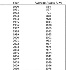
Table 3 - Average Assets to trade for each year Year Average Assets Alive
1990 554 1991 597 1992 701 1993 818 1994 970 1995 1043 1996 1030 1997 1069 1998 1093 1999 1065 2000 1001 2001 953 2002 957 2003 959 2004 987 2005 1029 2006 1042 2007 1039 2008 1049 2009 1046 2010 1076
Table 4 - Sample descriptive statistics
Price Volume n 5,030,358 5,030,358 Average 22.88 797,615 Standard Deviation 56.99 7,277,171 Median 16.69 142,500 Mode 10.00 1,000 Maximum 76,875 3,772,638,464 Minimum 0.0001 0
3.2. Pairs Formation and Trading Period
The methodology used for building the trading rules is the one proposed in GGR with the “wait one day rule” (the opening and close of a pair is delayed by one day to avoid the bid-ask bounce): There is a 250 working days period (the equivalent to a trading year) in which all possible pairs are formed and the sum of the squared deviations between the two normalized price series (prices are normalized to day 1 and include reinvested dividends) is taken. This is called the “closeness” measure.
19
Formula 1
|
!"# $ % & " ' ( " !"# $ % & " ' ( "
Then pairs are then ranked according to this measure (the smallest the closeness the better) and the Top “n” are taken into a period of 125 working days for trading (the equivalent to a six month trading period). The prices of the pairs are again normalized to the first day of this 125 day period and we start to monitor them. In this period if the spread between the assets is wider than 2 historical standard deviations (calculated in the 250 days training period) a Long/Short position is taken going short the asset that had the relative price increase and long the other. The trigger is calculated as following:
Formula 2
)!"** !| +2 ,&- .
!"# $ % & " ' ( " !"# $ % & " ' ( "
If at any time during the 125 day period the following condition is met:
Formula 3
20 Then the following position is set:
Formula 4
Long asset b, short asset a if 1 2
1 30
1 2
13 Long asset a, short asset b if 1 2
1 30
1 2
1 3
When and if prices cross again the position is unwind. If at the end of the 125 days trading period a position is opened or if one of the stocks in the pair is delisted then the position is unwind.
One difference in methodologies used is that GGR overlaps the period of 125 days of trading creating a number of portfolios that can be simultaneous trading the same pairs. The results presented here do not follow this methodology and the trading periods of 125 days do not overlap (they are 125 trading days apart) as shown in figure 1.
Figure 1 - Formation and Trading Period Representation
Formation Period: The price series of the assets are normalized to the first day and a measure of closeness (the sum of the square differences of the normalized prices) is taken for all possible pairs. Trading Period: The top “n” pairs, the ones with the smallest value of closeness are monitored and if the spread between the normalized prices (normalized to the first day of the trading period) is wider than the closeness measure plus 2 standard deviations (the standard deviation of the closeness measure taken from the formation period) a position is open.
Formation Period (250 Days)
Trading Period (125 Days) Formation Period (250 Days)
Trading Period (125 Days)
This is the simulation of the strategy of GGR and is used as a benchmark strategy to assess the value of the changes introduced. This strategy is mentioned as “GGR”.
21 3.3. Returns
A pair total return is computed as following:
Formula 5 "! 4 &5! 6, 7 ,89 : 6; 8 ;79 2 1 ,7 <= !"# $ ,> !& ; * ,8 !"# $ ,> !& ; * ;? <= !"# $ ; * ; * ;8 !"# $ ; * ; *
All the reported returns for the portfolios are computed on the capital that is actually invested at any time (GGR names this as “Fully Invested Returns”). So if just one of the top pairs is trading the daily mark to market is computed as being that pair daily return. The daily mark to market of the portfolio is computed as following:
Formula 6 !&$ " 4 &5! @ ∑ B , @C , @ : ; @ ; @C D E 1
, @ !"# $ > !& & $ = "! " " & , @C !"# $ > !& & $ = "! " " & 1 ; @ !"# $ * & $ = "! " " & ; @C !"# $ * & $ = "! " " & 1
3.4. Variations
One new rule that limits the number of days a pair is open (without convergence) is introduced with 5 variations: A variation for 15, 25, 50, 75 and 100 days limit is tested (the original strategy in GGR can be thought as a 125 day limit). If a pair is
22 closed because of this new rule then that specific pair will not trade anymore for that 125 day period. This ensures that the pairs traded in this variation are less or the same that the pairs traded in the GGR strategy and that they will be open for less or the same days.
Another introduction to the GGR strategy (that doesn’t affect the strategy in any way) is the classification of a pair in terms of volume shocks. In the pairs training period (consisting of the 250 working days prior to the trading period of 125 days) the average and standard deviation of volume is taken for each asset. This is the reference demand for that asset. Then, when a pair opens (on the day the trigger is activated), it’s classified in one of three ways:
• If the volume of one of the assets in the pair (and just one) is greater than the reference value the pair is classified has “Individual Shock”.
"$ FG H@ 0 4 HI ' G H@ J 4 HI K ! FG H@ 0 4 HI ' G H@ J 4 HI K )!5
• If the volume in the two assets is greater than the reference the pair is classified as “Common Shock”.
"$ FG H@ 0 4 HI ' G H@ 0 4 HI K )!5
• If none of the assets volume is greater than the reference the pair is classified as “No Shock”.
"$ FG H@ J 4 HI ' G H@ J 4 HI K )!5
H@ H 5L $ & " &
H@ H 5L $ & " &
4 H 4 $ ! # . 5L $ ! & 4 H 4 $ ! # . 5L $ ! &
23 For the reference value three situations are included: The reference is the average volume, the average volume plus 1 standard deviation and the average volume plus 2 standard deviations.
This methodology will allow a direct comparison of the changes introduced and the original strategy proposed in GGR so we can evaluate the impact of these new variations. Comparisons are made based on the Top 100 pair portfolios because they represent a more diversified portfolio and an increased data sample which provides lower statistical error.
24
IV. Results
4.1. GGR Results after 2002
GGR reported annualized returns of 11% for the period from July 1963 to December 2002. For the Top 20 portfolio that simulates the strategy used in GGR two distinct periods stand out from Table 5 and Table 6, the period until 2002 where annualized returns of 11.30% are achieved and the period from 2002 to 2010 when annualized returns (for the Top 20 strategy) drop to 5.60%.
Table 5 - Portfolio annualized returns for each strategy
This table presents the annualized returns of the different strategies: The one proposed in GGR, with a 15 day limit on the time pairs are trading (open), with a 25 day limit, a 50 day limit, a 75 day limit and with 100 day limit. Returns are calculated based on the invested capital and compounded on a monthly basis (monthly reinvestment of profits).
GGR 15 Days 25 Days 50 Days 75 Days 100 Days
Year Top 20 Top 100 Top 20 Top 100 Top 20 Top 100 Top 20 Top 100 Top 20 Top 100 Top 20 Top 100 1991 6.4% 5.8% 4.9% 7.2% 7.6% 9.7% 8.6% 6.7% 7.5% 6.2% 6.8% 6.0% 1992 8.7% 12.0% 7.2% 22.6% 13.2% 18.4% 9.1% 13.6% 8.2% 12.1% 8.7% 11.8% 1993 21.5% 17.8% 22.6% 19.5% 23.9% 26.0% 21.5% 20.6% 21.4% 18.8% 21.3% 18.3% 1994 9.5% 11.6% 3.2% 10.9% 11.0% 17.9% 8.7% 11.6% 11.1% 11.6% 9.2% 11.6% 1995 13.5% 14.6% 11.9% 20.9% 9.3% 17.3% 14.6% 18.1% 13.7% 16.3% 12.8% 14.9% 1996 0.2% 8.4% -3.0% 9.1% -2.7% 8.1% 2.1% 8.8% -0.2% 8.2% -0.1% 8.2% 1997 12.4% 11.8% 9.8% 17.6% 11.7% 20.1% 16.1% 15.1% 14.0% 13.3% 12.0% 11.7% 1998 11.9% 10.4% 6.4% 24.4% 23.4% 17.2% 18.5% 14.3% 10.6% 10.5% 11.7% 10.4% 1999 18.6% 18.2% 12.7% 28.2% 26.2% 26.1% 23.8% 20.9% 20.5% 19.0% 18.8% 18.4% 2000 15.2% 14.2% 13.0% 4.5% 18.9% 15.2% 14.7% 14.2% 15.0% 13.9% 15.1% 14.0% 2001 11.0% 13.8% 13.8% 16.9% 11.8% 16.4% 11.4% 15.1% 11.3% 14.2% 11.1% 13.9% 2002 8.7% 3.5% 5.2% 7.3% 13.3% 12.4% 11.7% 6.8% 8.7% 4.0% 9.0% 3.7% 2003 -2.4% 5.5% -0.2% 8.2% -6.7% 4.4% -4.4% 5.4% -3.0% 5.1% -2.4% 5.5% 2004 4.8% 6.7% 4.9% 14.1% 8.6% 12.6% 7.8% 8.4% 5.7% 7.3% 5.4% 6.8% 2005 1.4% 1.6% -1.1% 7.0% -2.9% 5.0% 3.4% 3.7% 1.1% 1.8% -0.2% 1.1% 2006 1.0% 7.6% -6.7% 6.1% 7.0% 6.8% 2.2% 7.8% 2.4% 8.4% 1.0% 7.5% 2007 3.3% 4.4% -0.2% 1.6% 7.7% 6.5% 5.3% 6.3% 4.4% 4.7% 3.6% 4.6% 2008 22.2% 23.4% 8.1% 10.7% 25.0% 27.6% 26.0% 25.9% 25.6% 25.6% 23.0% 23.6% 2009 4.4% 22.1% 13.9% 34.6% 6.7% 27.3% 6.4% 25.4% 6.4% 23.0% 4.3% 22.3% 2010 12.4% 10.1% 15.4% 4.9% 13.4% 10.0% 13.5% 10.9% 12.9% 11.3% 12.4% 10.0%
25
Table 6 – Portfolio annualized returns for the period between 1991 and 2002 and for the period
between 2003 and 2010
This table presents the annualized returns for 2 periods: One from 1 January 1991 to 31 December 2002 that overlaps with a segment of the period tested in GGR and a second one from 1 January 2003 to 31 December 2010. Returns are calculated based on the invested capital and compounded on a monthly basis (monthly reinvestment of profits).
GGR 15 Days 25 Days 50 Days 75 Days 100 Days
Period Top 20 Top 100 Top 20 Top 100 Top 20 Top 100 Top 20 Top 100 Top 20 Top 100 Top 20 Top 100 (1991-2002) 11.3% 11.8% 8.8% 15.5% 13.7% 16.9% 13.3% 13.7% 11.7% 12.3% 11.3% 11.8% (2003-2010) 5.6% 9.9% 4.0% 10.5% 7.0% 12.2% 7.2% 11.4% 6.6% 10.6% 5.6% 9.9%
From 2003 to 2007 returns were dramatically lower than the previous period. This suggests that something fundamental has change after 2002. This was the year when the revised paper, GGR, was published. The previous results, Gatev, Goetzmann and Rouwenhorts (1999) are from 1999 and the authors were surprised, throughout the revision of the earlier version, that the results (the excess returns) from 1999 to 2002 were still significantly positive. This may indicate that the market has acknowledged the results and corrected this statistical evidence by deploying similar strategies. On the other hand it could also signify that a latent risk factor was present for that period and that the reported excess returns aren’t has high has it was thought.
Also to be noted from Table 5 is that returns picked up from 2008 to 2011 with double digit figures and that 2008 was an extremely good year (in fact, the best year for the period under analysis) although US equity markets had one of the worst years in history (for example, the equity index S&P 500 lost 37% of its value). Another characteristic that stands out is that the Top 100 pair portfolio in the GGR strategy had 100% positive years. This track record is remarkably good.
26 4.2. Limiting the Time a Pair is Open
Table 7 presents the descriptive statistics for the pairs and Table 8 the monthly returns for the portfolios when we limit the days a pair is allowed to be trading (the pair is open).
Table 7 - Pairs Statistics
Descriptive statistics of the Pairs Returns following the strategy proposed by GGR. Pairs are formed over a 250 trading days period according to a minimum distance criteria, and then traded over the subsequent 125 trading days period. A pair is open (traded) on the day following the day on which the prices of the assets in the pair diverge by more than 2 historical standard deviations. The top pairs (Top 20 or Top 100) are the pairs with the least distance measures. Pairs are allowed to be open for a maximum of 125 days on the GGR strategy and for the indicated days (15, 25, 50, 75 or 100) in the remaining strategies.
GGR 15 Days 25 Days 50 Days 75 Days 100 Days
Top 20 Top 100 Top 20 Top 100 Top 20 Top 100 Top 20 Top 100 Top 20 Top 100 Top 20 Top 100 n 1219 6224 934 4694 1034 5238 1168 5920 1211 6156 1217 6221 Average 0.57% 0.61% 0.42% 0.46% 0.51% 0.55% 0.58% 0.64% 0.57% 0.61% 0.49% 0.61%
Standard Error (For the
Average) 0.14% 0.07% 0.09% 0.04% 0.11% 0.05% 0.12% 0.06% 0.13% 0.06% 0.14% 0.07%
Standard Deviation 4.96% 5.25% 2.86% 2.92% 3.39% 3.48% 4.26% 4.38% 4.61% 4.93% 4.99% 5.15%
Median 1.81% 1.84% 0.64% 0.56% 0.81% 0.78% 1.37% 1.36% 1.65% 1.69% 1.78% 1.81%
Skewness -2.06 -2.53 -0.27 -0.37 -1.03 -0.79 -1.57 -2.17 -1.61 -2.50 -2.03 -2.32
Kurtosis 9.28 21.15 1.92 3.16 5.96 8.94 6.53 26.22 6.01 27.76 9.20 18.94
Sharpe Ration (Risk Free
0%) 0.116 0.116 0.146 0.156 0.149 0.159 0.137 0.146 0.124 0.124 0.099 0.118
Negative Return Pairs 33% 34% 41% 41% 39% 40% 35% 37% 35% 35% 34% 34%
Average Trades Per Pair 1.59 1.63 1.22 1.23 1.35 1.37 1.52 1.43 1.58 1.61 1.58 1.63
Average Time Pairs are
27
Table 8 - Portfolio Statistics (Monthly Returns)
Descriptive statistics of the Pairs Returns following the strategy proposed by GGR. Pairs are formed over a 250 trading days period according to a minimum distance criteria, and then traded over the subsequent 125 trading days period. A pair is open (traded) on the day following the day on which the prices of the assets in the pair diverge by more than 2 historical standard deviations. The top pairs (Top 20 or Top 100) are the pairs with the least distance measures. Pairs are allowed to be open for a maximum of 125 days on the GGR strategy and for the indicated days (15, 25, 50, 75 or 100) in the remaining strategies.
GGR 15 Days 25 Days 50 Days 75 Days 100 Days
Top 20 Top 100 Top 20 Top 100 Top 20 Top 100 Top 20 Top 100 Top 20 Top 100 Top 20 Top 100 n 240 240 240 240 240 240 240 240 240 240 240 240 Average 0.73% 0.88% 0.58% 1.08% 0.89% 1.19% 0.87% 1.02% 0.78% 0.93% 0.73% 0.89% Standard Error
(For the Average) 0.10% 0.09% 0.14% 0.13% 0.13% 0.11% 0.11% 0.09% 0.11% 0.09% 0.10% 0.09% Standard Deviation 1.59% 1.34% 2.12% 2.03% 2.03% 1.69% 1.75% 1.46% 1.63% 1.39% 1.59% 1.36% Median 0.61% 0.74% 0.52% 1.00% 0.69% 1.01% 0.77% 0.89% 0.62% 0.75% 0.62% 0.73% Skewness 0.60 0.31 0.19 0.25 0.51 0.30 0.36 0.36 0.57 0.38 0.57 0.32 Kurtosis 1.55 1.73 1.58 2.96 1.12 1.53 0.31 1.97 1.33 1.73 1.46 1.67 Maximum 8% 5% 9% 11% 9% 7% 6% 6% 8% 5% 8% 5% Minimum -3% -4% -6% -7% -4% -5% 210% 245% 188% 223% 175% 213% Negative Return Months 33% 24% 36% 25% 32% 22% 33% 19% 32% 23% 33% 25%
It’s clear by Table 8 that the average monthly return (for the portfolio comprising of the 100 top pairs) increases no matter the limit in days that is applied, achieving the best performance for the 25 day limit. The monthly return ranges from 0.88% for the GGR strategy to 1.19% for the 25 day limit strategy (a range of 0.31%). Looking at the return characteristics of the pairs (Table 7) one can see that although the average return on the pair is lower on the 15 and 25 days limit (in comparison with the GGR results) there is a gain to be noted on the standard deviation side (in all the limits). The Sharpe ratio shows exactly that: It’s the lowest for the GGR strategy and the highest for the 25 days limit, just as the monthly returns. This suggests that this kind of strategy adds value without increasing the portfolio risk (it trades the same pairs for less time and/or avoids some trades) generating on the long term far greater returns as showed on Chart 3.
28
Chart 3
The chart shows how much would yield an investment on the different strategies (for the Top 100 Pairs portfolio) for the period from 1 January 1991 to 31 December 2010.
The chart is clear in showing that an investment on the GGR strategy would result in the lowest return of them all. This is also translated on the annualized return: For the Top 100 strategies GGR achieves an 11.02% annualized return for the whole period against a 15.02% return for the 25 day limit. So whateverlimit is imposed on the number of days a pair is trading there is an improvement on the strategies returns (with no increase in risk).
4.3. Volume Events
Table 9 shows that for every definition of volume event (average, average plus one standard deviation or average plus 2 standard deviations) the return of the pairs is the highest when the event happens on both assets, the lowest when the event is
0% 200% 400% 600% 800% 1000% 1200% 1400% 1600% 1800% 1 9 9 1 -0 1 -0 1 1 9 9 2 -0 1 -0 1 1 9 9 3 -0 1 -0 1 1 9 9 4 -0 1 -0 1 1 9 9 5 -0 1 -0 1 1 9 9 6 -0 1 -0 1 1 9 9 7 -0 1 -0 1 1 9 9 8 -0 1 -0 1 1 9 9 9 -0 1 -0 1 2 0 0 0 -0 1 -0 1 2 0 0 1 -0 1 -0 1 2 0 0 2 -0 1 -0 1 2 0 0 3 -0 1 -0 1 2 0 0 4 -0 1 -0 1 2 0 0 5 -0 1 -0 1 2 0 0 6 -0 1 -0 1 2 0 0 7 -0 1 -0 1 2 0 0 8 -0 1 -0 1 2 0 0 9 -0 1 -0 1 2 0 1 0 -0 1 -0 1 A cc u m u la te d R e tu rn ( F u ll y I n v e st e d )
Accumulated Returns of the Different Strategies - Monthly Compounded
15 Days Limit 25 Days Limit 50 Days Limit 75 Days Limit 100 Days Limit GGR Strategy
29 on one asset and when there is no event the average return falls between the two other classifications.
Table 9 - Pairs statistics (by volume)
This table presents the descriptive statistics for the top 100 pairs following the GGR strategy. Pairs are classified according to three distinct ways of defining a shock: In the first case a shock is defined as a day in which the volume (on the day the pair triggers) is greater than the average volume taken on the 250 days formation period, in the second case a shock is when the volume is greater than the average plus 1 standard deviation and in the third case a shock is when the volume is greater than the average plus 2 standard deviations.
Average Volume Average Plus 1 Standard
Deviation
Average Plus 2 Standard Deviations No Shock Individual Shock Common Shock No Shock Individual Shock Common Shock No Shock Individual Shock Common Shock n 1313 2889 2022 3662 2083 479 4724 1342 158 Average 0.58% 0.44% 0.87% 0.60% 0.50% 1.10% 0.61% 0.57% 0.89%
Standard Error (For the
Average) 0.14% 0.10% 0.12% 0.08% 0.12% 0.30% 0.07% 0.15% 0.67%
Standard Deviation 5.06% 5.11% 5.54% 4.85% 5.53% 6.67% 5.02% 5.54% 8.46%
Median 1.74% 1.76% 1.97% 1.82% 1.83% 2.08% 1.85% 1.78% 2.05%
Skewness -3.7 -2.1 -2.5 -2.7 -1.8 -3.8 -2.5 -1.5 -4.9
Kurtosis 43 10 23 24 9 38 20 6 42
Sharpe Ration (Risk
Free 0%) 0.115 0.086 0.157 0.124 0.091 0.165 0.121 0.104 0.106
Negative Return Pairs 34% 36% 32% 34% 35% 29% 34% 35% 30%
Average Trades Per
Pair 1.14 1.27 1.28 1.37 1.24 1.16 1.47 1.17 1.09
Average Time Pairs are
Open (in Months) 1.48 1.53 1.46 1.49 1.54 1.36 1.48 1.56 1.33
Cross Pairs 52% 49% 52% 51% 49% 54% 51% 48% 53%
End of Period 48% 51% 48% 49% 51% 46% 49% 52% 47%
This regularity is also observed in the sharpe ratio with the exception of when the volume event is defined as the average plus 2 standard deviation, although the error is too high to draw any conclusion (the sample of pairs with volume events in both pairs becomes too small, n=158). These results confirm the findings of Engelberg, Gao and Jagannathan (2009) that pairs opening after news that affected both assets exhibit superior returns and that when news affected just one of the assets returns were under average. This opens the door for the possibility that market participants have acknowledged these high return pairs and use this
30 information to form a conditional filter on the opening of the pairs (opening pairs only if there are shocks that affect both assets). It’s also important to note that this volume information is a good proxy for idiosyncratic or common shocks and that it’s available before the opening of the pair (pairs are open one day after the trigger fires). It is also as common and as cheap as the price data.
31
V. Conclusion
The results show that the simple relative value model presented by GGR has margin to be improved through simple rationales coherent with the main idea.
The limit introduced on the maximum days a pair is open improves the risk return characteristics no matter what limit is imposed which appears to support the rationale that a convergence must be observed in a short period of time. We can also conclude that is best to avoid pairs that trigger around abnormal volume changes in one of the assets.
It’s fair to expect that market participants took and take these strategies to levels of sophistication beyond what is tested and presented here and that those returns can prove to be resilient to the explicit and implicit costs that Do and Faff (2011) have analyzed. With just the introduction of a limit of 25 days on the time a pair is open would add 5% on a yearly base to the original (GGR) strategy of a portfolio comprising of the Top 100 pairs.
It’s plausible to think that these modifications and others are employed by some more or less sophisticated market participants and that the returns generated can challenge the weak form of the efficient market hypothesis. It’s also possible that with the high frequency price data that is available today this strategies are taken to an intraday level where the price divergences could prove to be momentarily larger and thus the strategy prove to be more profitable.
But some fundamental questions still persist: Market participants often employ strategies with some type of risk management control. Pairs trading, as proposed by
32 GGR is lacking such characteristic. Other questions relate to the extent to which returns are indeed the result of liquidity provision or how much close are the reference values used by GGR, namely the training and trading period and the 2 standard deviation trigger, to the values that market participant’s really use.
It’s still unclear the real merits of pairs trading and what results different formats of this strategy would yield. What we can conclude is that the excess returns presented here are large enough to pursue further investigation.
33
References
Andrade, S., Di Pietro, V., Seasholes, M. 2005. Understanding the profitability of pairs trading. UC Berkeley Working Paper
Do, Binh and Faff, Robert. 2010. Does Simple Pairs Trading Still Work?. Financial Analysts Journal, Vol. 66, No. 4, pp. 83-95, 2010
Do, Binh and Faff, Robert. 2011. Are Pairs Trading Profits Robust to Trading Costs? Elliott, Robert, Van Der Hoek, John and Malcolm, William. 2005. Pairs trading. Quantitative Finance, Vol. 5, Issue 3, 2007
Engelberg, Joseph, Gao, Pengjie and Jagannathan, Ravi. 2009. An Anatomy of Pairs Trading: The Role of Idiosyncratic News, Common Information and Liquidity
Fama, Eugene. 1970. Efficient Capital Markets: A Review of Theory and Empirical Work. Journal of Finance
Gatev, Evan, Goetzmann, William N. and Rouwenhorst, K. Geert. 2006. Pairs Trading: Performance of a Relative Value Arbitrage Rule. Yale ICF Working Paper No. 08-03
Nath, Purnendu. 2003. High Frequency Pairs Trading with U.S. Treasury Securities: Risks and Rewards for Hedge Funds
Papadakis, G., and Wysocki, P. 2008. Pairs trading and accounting information Richards, Anthony J. 1999. Idiosyncratic Risk An Empirical Analysis, with Implications for the Risk of Relative-Value Trading Strategies. IMF Working Paper No. 99/148 SEC Halts Short Selling of Financial Stocks to Protect Investors and Markets. Available in http://www.sec.gov/news/press/2008/2008-211.htm
Vidyamurthy, Ganapathy. 2004. Pairs Trading: Quantitative Methods and Analysis. Hoboken: Wiley