On Statistically Estimated Optimistic
Delivery in Wide-Area Total Order
Protocols
Jos´e Mocito
Ana Resp´ıcio
Lu´ıs Rodrigues
DI–FCUL
TR–06–22
September 2006
Departamento de Inform´atica
Faculdade de Ciˆencias da Universidade de Lisboa
Campo Grande, 1749–016 Lisboa
Portugal
Technical reports are available athttp://www.di.fc.ul.pt/tech-reports. The files are stored in PDF, with the report number as filename. Alternatively, reports are available by post from the above address.
On Statistically Estimated Optimistic Delivery in Wide-Area Total Order
Protocols
∗Jos´e Mocito
Ana Resp´ıcio
University of Lisbon
{jmocito,respicio,ler}@di.fc.ul.pt
Lu´ıs Rodrigues
Abstract
Total order broadcast protocols have been successfully applied as the basis for the construction of many fault-tolerant distributed systems. Unfortunately, the implemen-tation of such a primitive can be expensive both in terms of communication steps and of number of messages ex-changed. To alleviate this problem, optimistic total order protocols have been proposed. This paper addresses the problem of offering optimistic total order in geographically wide-area systems. We present a protocol that outperforms previous work, by minimizing the average latency of the op-timistic notification.
1. Introduction
Total order broadcast protocols have been successfully applied as the basis for the construction of many fault-tolerant distributed systems, from clock synchronization [8] to database replication [5, 2]. The purpose of such a pro-tocol is to provide a communication primitive that allows processes to agree on the set of messages they deliver and also on their delivery order.
Unfortunately, the implementation of such a primitive can be expensive both in terms of communication steps and of number of messages exchanged. This problem is exacer-bated in wide-area networks, where the performance of the algorithm may be limited by the presence of high-latency links. To alleviate this problem, optimistic total order proto-cols have been proposed [9, 10]. Such protoproto-cols provide to the application an early indication of the estimated defini-tive total order. The application can use this estimate to perform a number of actions optimistically, which are later committed when the final definitive order is established. The goal is to execute some application steps in parallel with the communication steps of the total order algorithm.
∗This work has been partially supported by the project IST-STREP
004758, GORDA: Open Replication of Databases.
To the best of our knowledge, the protocol that is able to offer the smaller latency in the optimistic delivery notifica-tion in wide-area networks has been proposed by Sousa et
al. in [9]. The protocol is an optimistic variant of the well known sequencer based total order algorithm.
In this paper we show that the algorithm used in [9] fails to offer the optimal average latency of optimistic deliveries. Departing from this observation we discuss how the opti-mal delays can be computed and, subsequently, propose an efficient heuristic to approximate the optimal result in an cost-effective manner. The resulting protocol is evaluated and compared with the original protocol.
This paper is structured as follows. In Section 2 we vide an overview of the optimistic total order protocol pro-posed in [9]. Section 3 highlights why the strategy followed in that protocol is suboptimal and discusses the optimal so-lution. An heuristic that approximates the optimal solution is presented in Section 4. An evaluation of the resulting al-gorithm is given in Section 5. Finally, in Section 6 we pro-vide the concluding remarks.
2. Statistically Estimated Total Order
In this section we provide a brief overview of the opti-mistic total order presented in [9]. This protocol, that we will refer to as SETO (Statistically Estimated Total Or-der), was developed specifically targeting wide area net-works and was inspired by the ideas originally presented in [6], where the spontaneous ordering properties of local area networks are used to provide optimistic deliveries in sequencer-based total order protocols.
2.1. Overview
The notion of optimistic total order was first proposed in the context of local-area broadcast networks [6]. In many of such networks, the spontaneous order of message reception is the same in all processes. Moreover, in sequencer-based total order protocols the total order is usually determined
s
2 ms
a b
10 ms
Figure 1. Local and wide-area links.
by the spontaneous order of message reception in the se-quencer process. Based on these two observations a process may estimate the final total order of messages based on its local receiving order and, therefore, provide an optimistic delivery as soon as a message is received from the network. Such approach is unfeasible in large-scale networks. The long latency in wide-area links causes different processes to receive the same message at different points in time. Con-sider the topology depicted in Figure 1. Assume that pro-cess a multicasts a message m1and that, at the same time,
the sequencer s multicasts a message m2. Clearly, the
se-quencer will receive m2< m1, given that m1would require
12ms to reach the sequencer. On the other hand, process b will receive m1< m2, as m1will take only2ms to reach b
while m2will require12ms. From this example, it should
be obvious that the spontaneous total order provided by the network at b is not a good estimate of the observed order at the sequencer.
To address the problem above, [9] proposed to introduce artificial delays in the message reception to compensate for the differences in the network delays. It is easier to describe the intuition of the protocol by using a concrete example. Consider again the network of Figure 1. Assume also that we are able to provide to each process an estimate of the network topology and of the delays associated with each link. In this case, b could infer that message m1would take
10ms more to reach s than to reach b. By adding a delay of 10ms to all messages received from a, it would mimic the reception order of a’s messages at s. A similar reasoning could be applied to messages from other processes.
2.2. The SETO algorithm
We now provide a precise description of the algorithm (Figure 2) used in the original SETO protocol to estimate the delays that should be added to each message. The algo-rithm is the same that has been published in [9] and is de-picted here for self-containment. We recall that the rationale behind the solution is to make every process equidistant in respect to the sequencer. This way, the spontaneous order observed in the sequencer will be the same as the optimistic
1:Initialization:
2: g ← 0 {Global sequence number}
3: l ← 0 {Local sequence number}
4: R ← ∅ {Messages received}
5: S ← ∅ {Sequence numbers}
6: O ← ∅ {Messages opt-delivered}
7: F ← ∅ {Messages fnl-delivered}
8: delay[1..n] ← 0
9: r delay[1..n] ← 0 {Delays requested to the sequencer}
10: procedureT O multicast(m)
11: R multicast(DATA(m, max(delay[] − delay[seq]))
12: uponR deliver(DATA(m, d)) do 13: R ← R ∪ {(m, d, now + delay[m.sender])} 14: upon∃(m, d, t) ∈ R : now ≥ t ∧ m /∈ O ∧ m /∈ F do 15: opt delivery(m) 16: O ← O ∪ m 17: ifp = seq then 18: g ← g + 1 19: R multicast(SEQ(m, g)) 20: r delay[m.sender] ← d
21: delay[p] ← max(rdelay[])
22: uponR deliver(SEQ(m, s)) do 23: S ← S ∪ {(m, s, now)} 24: upon∃(m, d, o) ∈ R : (m, l + 1, t) ∈ S ∧ m /∈ F do 25: f nl delivery(m) 26: if∃(m′ , d′ , o′ ) ∈ R : (m′ , l, t′ ) ∈ S then 27: ∆ ← (t − t′ ) − (o − o′ ) 28: if∆ > 0 then 29: adjust(m′ .sender, m.sender, ∆) 30: else 31: adjust(m.sender, m′ .sender, |∆|) 32: l ← l + 1 33: F ← F ∪ {m} 34: procedureadjust(i, j, d) 35: v ← (delay[i] × α) + (delay[i] − d) × (1 − α) 36: ifv ≥ 0 then 37: delay[i] ← v 38: else 39: delay[i] ← 0 40: delay[j] ← delay[j] + |v|
Figure 2. Original SETO algorithm.
order artificially induced in each process.
In simple terms, the algorithm provides a multicast prim-itive (line 10) that ensures regular total order delivery in a group of processes. When a message arrives from the net-work (line 12) it is queued for optimistic delivery (line 13) after a certain period of time, which was previously esti-mated to approximate the spontaneous order as seen by the sequencer process. When that time comes (line 14) the mes-sage is optimistically delivered (line 15). When this hap-pens in the sequencer process, the sequence number to that message is also generated (line 18) and is multicast to every process (line 19). Upon reception of the sequence num-ber (line 22) the message is authoritatively delivered to the application. This description is obviously simplistic, as it omits the parts that deals specifically with the estimation of the delays to apply to optimistic message deliveries. Those parts will now be described.
First we will deal with the estimation of the delays on all processes other than the sequencer. When messages are
received from the network their optimistic delivery time is recorded (line 13). Also, when the sequence numbers are received from the sequencer, the time is also recorded (line 23). During the authoritative delivery of messages both recorded times are used to compare the optimistic and au-thoritative order of the current a last delivered messages (line 27). This comparison then determines the adjustments that must be made to the artificial delays (lines 28-31).
The second part is the estimation of delays in the se-quencer process. This procedure cannot be the same as used in other processes because the basic delay estimation mech-anism uses the sequencer itself as a reference to compen-sate distance divergences between processes. The way the protocol copes with this problem is to make the sequencer delay its own messages by the maximum amount of time a message it sent takes to reach any other process. Consider the network depicted in Figure 3(a). The messages sent by the sequencer s would have to be delayed by9ms which corresponds to the maximum time a message sent from s takes to reach any other process (in this case p2). Note that,
in the algorithm, instead of having the sequencer actively determine the maximum delay to any process, each process suggests a delay based on the delays it is applying to mes-sages from other processes (line 11). The sequencer then chooses the suggestion that has the highest value (line 21).
In the next section we address the limitations of SETO and discuss how it can be improved.
3. On the Latency of SETO
Let δij denote the latency of the optimistic delivery of
messages from process piat process pj. Figure 3(b)
illus-trates the values of δji for all processes, as the result of ap-plying the original SETO algorithm to the topology of Fig-ure 3(a). In this case, given that the sequencer (p3) delays
its own messages, we have δ31= 7, δ23 = 9 and δ33 = 9. If
all processes transmit at the same rate, we have an average message latency of7.66ms as a result of this configuration. The question addressed in this paper is the following: is this set of optimistic delivery latencies optimal?
Figures 3(c) and 3(d) depict alternative sets of delivery latencies for the optimistic delivery that would also respect the total order. Again, considering that all processes send at the same rate, the average latency derived from config-uration of Figure 3(c) is9.66ms and that of Figure 3(d) is 7.00ms. Thus, it is clear that SETO does not offer the opti-mal latency of optimistic delivery. Note that it is possible to find many other assignments that would also provide a basis for totally ordering the messages. In fact, any delay assign-ment that respects the following constraint can be used to establish a total order:
δki−δ i l= δ j k−δ j l ∀i, j, k, l ∈ 1, ..., N (1) δi
k− δil is the amount of time between the reception of
messages from pk and plat process pi. This value may be
negative – whenever pi receives the message from plafter
the one from pk. Equation (1) states that given a pair of
pro-cesses pk and pl, k, l= 1, ..., N , the time interval between
the reception of messages from these processes is always the same, independently of the receiver we consider.
Consider the permutation that defines the total order of messagesQ=< π1, ..., πn >, where πk ∈ {1, ..N } is the
index of the process sending the message to be received in the k-th position. Another way to express equation (1), is the following: δiπ1+k−δ i π1= δ j π1+k−δ j π1∀i, j ∈1, ..., N , k ∈ 1, ..., N − 1. (2)
This equation expresses that the time interval between the reception of any message πk+1and the reception of the
first message in the total order π1is the same at all the
pro-cesses. Obviously, in equation (2) the time differences un-der comparison are always positive, in opposition to those in equation (1). Clearly, all the assignments of Figure 3 re-spect the constraint above and are, therefore correct. Still, the same question remains: is the configuration from Fig-ure 3(d) the optimal?
3.1. Optimal Assignment
In this paper we seek solutions that minimize the overall average latency (OAL) of all optimistic deliveries, denoted ∆avg. Let ri be the rate at which process pi sends
mes-sages.∆avg is defined as:
∆avg = PN i,j=1riδij NPN j=1rj (3)
Minimizing the overall average latency of all optimistic deliveries is equivalent to Minimize the Overall Latency (MOL) and this problem can be mathematically formulated in linear programming as:
MOL: min N X i,j=1 riδij (4) s.t.: δ1i−δ 1 i+1= δ j i−δ j i+1, i= 1, ..., N − 1, j = 2, ..., N (5) δji ≥0, i, j= 1, . . . , N. (6)
Equation (4) states the objective function to be mini-mized: the weighted sum of all the latencies. Equation (5) ensures that the latencies under decision will give rise to a total order. It can be easily derived from equation (1) that,
9 ms 7 ms 5 ms p3(S) p1 p2 (a) 9 ms 7 ms 5 ms p3(S) p1 p2 [5, 7, 7] [7, 9, 9] [7, 9, 9] (b) 9 ms 7 ms 5 ms p3(S) p1 p2 [11, 13, 7] [13, 15, 9] [7, 9, 3] (c) 9 ms 7 ms 5 ms p3(S) p1 p2 [3, 5, 7] [5, 7, 9] [7, 9, 11] (d) Figure 3. SETO latency and alternative configurations.
as we stated above, it assures total order. Finally, equation (6) ensures that all the latencies are non-negative.
Let ωji denote the network delay of messages from pro-cess pi to process pj and let xji denote the delay these
messages should suffer to accomplish the corresponding la-tency δji, i, j = 1, ..., N . Consequently, by rewriting δji as δij = ω j i + x j i, and considering x j
i as the new decision
variables, the MOL can be reformulated as:
min N X i,j=1 rixji (7) s.t.: (ω1 i+ x 1 i) − (ω 1 i+1+ x 1 i+1) = (ω j i + x j i) − (ω j i+1+ x j i+1), i= 1, ..., N − 1, j = 2, ..., N (8) xji≥0, i, j= 1, . . . , N. (9)
In this new formulation, equation (7) states the objective function to be minimized: the weighted sum of the delays to impose to all the messages. Equation (8) ensure total order, while equation (9) guarantees for the non negativity of the delays.
This problem has N2 decision variables and(N − 1)2
constraints of type (8). Instances of the MOL problem can be solved using a solver of Linear Programming models, such as ILOG CPLEX [1]. In our case, we used ILOG CPLEX 9.0 to obtain the optimal solutions of all the in-stances under testing. When applying the solver to the topology of Figure 3(a) we obtained the delays depicted in Figure 3(d) which correspond to the optimal solution.
4. Fast SETO
As noted in the previous section, it is possible to derive the optimal solution using a solver of linear programming models. Unfortunately, it may be unpractical to install and execute such solver in each protocol stack of every process
of the distributed system. Therefore, in this section we pro-vide a heuristic to calculate the delays to be applied to each incoming message, that approximates the optimal solution.
This section also provides a complete protocol that gath-ers the topology information required for the solver or the heuristic and provides an optimistic delivery that outper-forms the original SETO algorithm described in Section 2.2.
4.1. Rationale for the Heuristic
Our heuristic works as follows. We incrementally build a network by adding one process at a time. The first process to be added defines the first message in the total orderQ, named π1 (see Section 3). This first process has complete
freedom to set the delay it imposes on its own messages (which may be zero).
Whenever another process is added to the network it tries to set itself as close as possible to π1 in the total orderQ,
subject to the restrictions from equations (2) and (9). Note that the later a process is inserted in the network, the larger the set of constraints it has to satisfy; therefore, it is likely that later processes may be required to add longer delays to their own messages.
A key point in the heuristic is the order by which pro-cesses are inserted in the network. To define this order, we use the following insight. Consider process pk. When
pro-cess pk is added to the network, the delay that this process
has to impose to its own messages xkk depends of the
con-straints imposed by processes p1, . . ., pk−1previously
in-serted. Consider now the next process to be added to the system pk+1 and ωkk+1the latency of the link between pk
and pk+1. If xkk > ω k+1
k , pk+1will be forced to impose
a delay to its own messages of at least ωkk+1− xk k. This
will happen if pkis very close to pk+1and is forced to
im-pose a long delay to its own messages. This means that the closer a process is to other processes, the more likely it is to influence the delays imposed on the messages from those processes. Thus, processes that are closer to other processes should impose the minimum delays to their own messages.
Since processes that are inserted earlier in the network are more likely to impose smaller delays (as they have less con-straints to satisfy), these processes should be the ones to be inserted first. The heuristic described in the next para-graphs, uses a precise metric to capture the fuzzy notion of “closeness” introduced here.
The paragraph above explains the negative impact of set-ting xkksuch that xkk > ωkk+1. It is interesting to note how-ever, that it may not be always desirable to set xkk = 0. In fact, by setting xkk = 0, we are forcing pk+1 to set
xk+1k+1 = ωkk+1. So, there is a trade-off between the delay process pkimposes on its own messages and the delay that
other processes will later have to impose on their own mes-sages. In the heuristic below we also specify a concrete formula to capture this balance.
4.2. Optimal Delay Approximation
The specification of the heuristic is presented in Figure 4. The procedure works in a stepwise fashion, computing de-lays for one process at a time.
First, let us introduce the notation used. A process in the group is denoted by pi, where i is the process identifier. The cost metric used provides a measure of the distance each process has to all the remaining processes. Let ωij denote the latency of the transmission delay between processes i and j, and rithe rate at which process pi sends messages.
The cost ciassociated with process pi is given by the
fol-lowing expression: ci= PN j=1ω j i ri
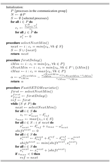
The heuristic considers a group of N processes where each process holds complete information about all the trans-mission delays of all processes. This information can be expressed in a N × N matrix that we call Ω, as illus-trated in Figure 5, where the rows are the processes and the columns are the transmission delays of messages from each of the corresponding processes, i.e., positionΩ(i, j) holds the transmission delay ωji of messages from process j to process i. Every process also maintains a similar ma-trix χ, holding the delays each process applies to messages from the others (including themselves) from which the final delay matrix∆ can be derived. We recall that the final de-lay δji is defined as δ j i = ω j i + x j
i. Figure 5 illustrates the
values of these matrices in the optimum configuration for the topology of Figure 3(a).
The heuristic proposed runs on an average of O(N2)
steps (where N is the number of processes in P ). The main cycle introduces a process at each iteration which is done exactly N− 1 times. Each of these iterations includes four cycles each of which executes O(♯S) iterations, with ♯S go-ing from1 to N .
Initialization:
P {processes in the communication group} N ← #P S ← ∅ {selected processes} for alli ∈ P do ci← PN j=1ωij ri for allj ∈ P do xji← 0
procedureselectN extMin()
next ← i : ci= min{ck, ∀k /∈ S}
S ← S ∪ {next}
returnnext
proceduref irstDelay()
iMin ← i : ci= min{ck, ∀k ∈ P }
iN extMin ← i : ci= min{ck, ∀k ∈ P \ {iMin}}
iMax ← i : ci= max{ck, ∀k ∈ P }
α ← ωiN extM in
iM in −
ωiN extM iniM in ×(ciNextMin−ciMin) ciMax−ciMin
returnα
procedureF astSET OHeuristic() f irst ← selectN extMin() xf irst
f irst← f irstDelay()
ref ← f irst
while(S 6= P ) do
next ← selectN extMin()
for alli ∈ S do
zi← ωinext− δ
i ref
zmax← max{zi, i ∈ S}
for alli ∈ S : i 6= next do
xi
next← δrefi + zmax− ωinext
shif tnext← 0 for alli ∈ S do xnext i ← δrefnext+ δ ref i − δ ref ref− ω next i
shif tnext← min(shif tnext, xnext
i ) for alli ∈ S do xnext i ← x next i + |shif t next| ifzmax< 0 then ref = next Figure 4. Heuristic.
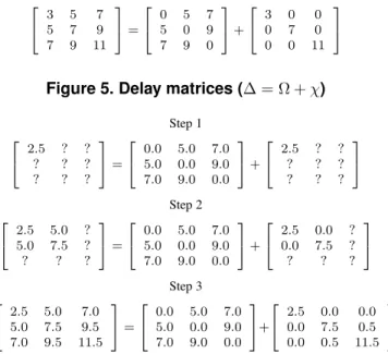
We now illustrate its execution step by step for the topol-ogy of Figure 5. In this example, we assume that all pro-cesses transmit at the same rate. The algorithm is initiated by computing the costs for each process: c1= 7 + 5 = 12,
c2 = 9 + 5 = 14 and c3 = 7 + 9 = 16. Thus, the first
process to be added to the network is process p1. Node p1
has no constraint in the delay it may impose to its own mes-sages. Therefore, it uses the formula depicted in Figure 4 (line 17) to set this value. In the case of the current ex-ample, the resulting value is2.5. This concludes Step 1 of the algorithm. The value of the matrices after this step are depicted in Figure 6.
On Step 2, the next process with the lowest cost is pro-cess p2. We first discover the delay x22that p2needs to
im-pose on its own messages. Note that we want to minimize x22subject to the constraint δ21− δ1
1 = δ22− δ21. Given that a
message sent by p2at time0 is received at p1at time5, we
have δ12− δ11= 5 − 2.5 = 2.5. Also, given that a message
sent by p1at time0 is received at p2at time5, to respect
2 4 3 5 7 5 7 9 7 9 11 3 5= 2 4 0 5 7 5 0 9 7 9 0 3 5+ 2 4 3 0 0 0 7 0 0 0 11 3 5
Figure 5. Delay matrices (∆ = Ω + χ)
Step 1 2 4 2.5 ? ? ? ? ? ? ? ? 3 5= 2 4 0.0 5.0 7.0 5.0 0.0 9.0 7.0 9.0 0.0 3 5+ 2 4 2.5 ? ? ? ? ? ? ? ? 3 5 Step 2 2 4 2.5 5.0 ? 5.0 7.5 ? ? ? ? 3 5= 2 4 0.0 5.0 7.0 5.0 0.0 9.0 7.0 9.0 0.0 3 5+ 2 4 2.5 0.0 ? 0.0 7.5 ? ? ? ? 3 5 Step 3 2 4 2.5 5.0 7.0 5.0 7.5 9.5 7.0 9.5 11.5 3 5= 2 4 0.0 5.0 7.0 5.0 0.0 9.0 7.0 9.0 0.0 3 5+ 2 4 2.5 0.0 0.0 0.0 7.5 0.5 0.0 0.5 11.5 3 5
Figure 6. Execution of the heuristic.
matrices after Step 2 are depicted in Figure 6.
In the final step, we need to add the last process p3. Note
that the value of x33needs to be minimized having now two
constraints to satisfy. When looking at the reception order at process p1, it is possible to see that messages from p3
have to be delivered4.5ms after messages from p1. When
looking at the reception order at process p2, it is possible to
see that messages from p3have to be delivered4ms after
messages from p1. The limiting factor is therefore the
in-terval at p1, that forces p3to set x33= 11.5, resulting in the
final matrices depicted in Figure 6.
Note that, in this case, the final average cost for the con-figuration derived from our heuristic is∆avg = 7.16 which is within3% of the optimum computed by the solver. In the evaluation we present results for other networks as well.
4.3. Algorithm
We now present an augment version of the SETO algo-rithm, that we have named Fast SETO, that can work with the heuristic or by calling a solver to obtain the minimum optimistic latency. The complete Fast SETO algorithm is specified in Figure 7. The algorithm works in four steps. In the first step, every process collects round-trip delays from all the other processes and estimates the corresponding transmission delays. This step is omitted in the algorithm specification for clarity sake, given there are multiple ways of collecting round-trip estimations and that procedure is orthogonal to the main algorithm. For instance, if TCP is used as the underlying transport protocol, the round-trip es-timation could be extracted from the TCP implementation
1:Initialization:
2: P ← p1, ..., pn{Process group}
3: delay[1..n] ← 0 {Delay applied to messages}
4: tdelay[1..n] ← 0 {Transmission delays to the process}
5: ctdelay[1..n][1..n] ← 0 {Complete transmission delay matrix}
6:procedurecomputeDelays()
7: {computes delays using the solver or the heuristic}
8:uponR deliver(DELAY(new delay[]) do
9: ifsender = seq then
10: ctdelay[new delay.sender] = new delay
11: else
12: delay = new delay
13: procedureupdateDelays()
14: R unicast(seq,DELAY(tdelay))
15: uponallDelaysGathered() do
16: c delay ← computeDelays()
17: for allpi∈ P do
18: R unicast(pi,DELAY(c delay[pi])
19: procedureT O multicast(m) 20: R multicast(DATA(m)) 21: uponR deliver(DATA(m) do 22: R ← R ∪ {(m, now + delay[m.sender])} 23: upon∃(m, d, t, md) ∈ R : now ≥ t ∧ m /∈ O ∧ m /∈ F do 24: opt delivery(m) 25: O ← O ∪ m 26: ifp = seq then 27: g ← g + 1 28: R multicast(SEQ(m, g)) 29: uponR deliver(SEQ(m, s)) do 30: S ← S ∪ {(m, s, now)} 31: upon∃(m, d, o) ∈ R : (m, l + 1, t) ∈ S ∧ m /∈ F do 32: f nl delivery(m) 33: l ← l + 1 34: F ← F ∪ {m}
Figure 7. Fast SETO algorithm.
without any extra cost. In the second step, all processes send the gathered delay information to a specific process. This process’s identity can be easily derived from the group membership; for instance, it can be the process with the smallest identifier. The process gathers all the delay infor-mation and computes the optimal delay when a solver is available, or approximates the optimal solution using the heuristic described in Section 4.2 when the use of a solver is impractical. Finally, it sends to each process in the group the corresponding line in the delay matrix, which holds the delays that must be enforced by that specific process.
Our algorithm clearly differs from the original SETO al-gorithm by requiring complete knowledge of the transmis-sion delays between all processes, which translates into the exchange of distance vectors between all nodes. The origi-nal SETO requires no such information, making use of only local clock values to determine the artificial delays. How-ever, our proposal significantly improves the overall average latency of the system, as will be shown in the next section.
5. Evaluation
In this section we evaluate our proposed algorithm against the optimal delay assignment and the original SETO algorithm. The evaluation tests were performed in a sim-ulated environment that consists of a network topology, transmission rates associated with each node and three mod-els that describe the three algorithms at stake: optimal as-signment, original SETO and Fast SETO using the heuris-tic. The network topologies used were generated with BRITE [3]. The tests were performed in networks with 30 nodes (10 nodes for the last evaluation test) that where ran-domly placed in a topological space.
5.1. Network Plane Size
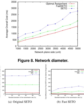
We first compare the performance of the optimal assign-ment, original SETO and Fast SETO when the network plane size is changed. BRITE allows for the definition of the plane size by specifying the dimension of one side. In the experiments performed we made this side vary between 1000 and 5000 units. For each space dimension 20 network topologies were generated, and the results shown are aver-age values of the observations on those networks. Also, in the original SETO algorithm a randomly selected sequencer was used.
The results are depicted in Figure 8. The explanation for these results lies in the way the original SETO algorithm determines the delay imposed by the sequencer to its own messages, which is equal to the longest link that reaches the sequencer. This value then conditions the adjustments in the remaining nodes and produces the observed results. The results also show the improvements obtained by Fast SETO in regard to the original algorithm and also its prox-imity to the optimal solution. In the experiments, the orig-inal SETO algorithm was, on average, 66% to 114% worst than the optimal assignment. Fast SETO with the heuristic was, on average, 16% to 33% worst than the optimal assign-ment, which shows the significant gains obtained by using our proposed algorithm.
5.2. Process Transmission Rates
We now compare the performance of the optimal assign-ment, original SETO and Fast SETO when the transmission rates of the processes in the network are changed. This time we set the topological space to a constant value. Each exper-iment consisted in generating 20 different topologies where all nodes exhibited an average transmission rate of 300 mes-sages per second, with a predefined variance. The standard deviation of the transmission rates for each experiment was made variable between 0% to 100%. As in the previous
0 500 1000 1500 2000 2500 3000 3500 1000 1500 2000 2500 3000 3500 4000 4500 5000
Average Overall Cost (ms)
Network plane side (unit) Optimal Assignment
FastSETO SETO
Figure 8. Network diameter.
0 100 200 300 400 500 600 0 20 40 60 80 100
Cost difference from SETO to the Optimal Assignment Standard deviation of the transmission rate (%) Min Average Max
(a) Original SETO
0 100 200 300 400 500 600 0 20 40 60 80 100
Cost difference from Fast SETO to the Optimal Assignment Standard deviation of the transmission rate (%)
Min Average Max
(b) Fast SETO Figure 9. Relative rates.
experiment, the sequencer for the original SETO algorithm experiments was randomly selected.
Figures 9(a) and 9(b) hold the results for both the exper-iments comparing the original SETO with the optimal as-signment and Fast SETO with also the optimal asas-signment, respectively. Each figure presents the results as differences from each algorithm to the optimal assignment. The three lines presented in each figure are the minimum, maximum and average values observed from all the 20 topologies for each standard deviation value.
As expected, the average overall cost of the Fast SETO algorithm suffers less variation than the original SETO al-gorithm. The reason for this is that Fast SETO takes into account the transmission rates when computing the artifi-cial delays. The original SETO algorithm makes no use of this information, which makes its results more dependent of the specific topology where it is executing.
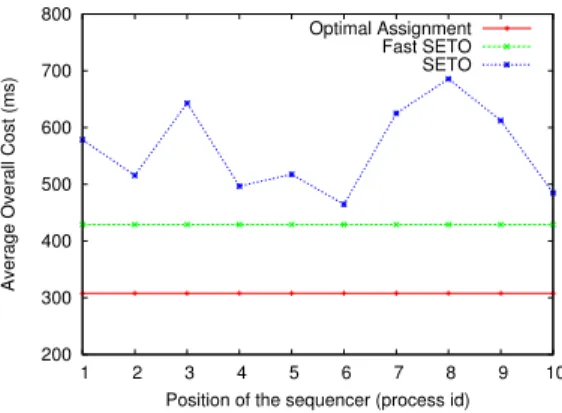
5.3. Sequencer Position
The final evaluation compared the three algorithms: original SETO, Fast SETO and optimal assignment, in re-gard to the sequencer position in the original SETO algo-rithm. This “position” refers to the identifier of the node that performs the sequencer role. For the experiments we used a network of 10 nodes with transmission rates uni-formly distributed by all nodes and varying from 0 to 100
200 300 400 500 600 700 800 1 2 3 4 5 6 7 8 9 10
Average Overall Cost (ms)
Position of the sequencer (process id) Optimal Assignment Fast SETO SETO
Figure 10. Sequencer’s position.
messages per second. For each sequencer position 20 net-work topologies where generated. The same 20 netnet-work topologies where used in all tests for the different positions, and the average overall cost of the 20 observations was used to produce the results presented in Figure 10.
The lines that represent the optimal assignment and the Fast SETO algorithm are obviously straight lines, because both algorithms results are not dependent of the sequencer position. As for the original SETO line, it is quite irregular and varies from little below500ms to almost 700ms, and always stays above the other algorithms lines. This clearly shows how the results of this algorithm depend on the se-quencer position for a given network topology.
For this, the first step of the heuristic we propose for the Fast SETO algorithm may be quite useful for improving the results of the original SETO algorithm by helping to choose the best sequencer location.
6. Conclusion
In this paper we have studied the problem of minimizing the latency of optimistic delivery in total order protocols for wide-area networks. The contributions of the paper are the following. Firstly, we have shown that previous solutions do not provide the optimal solution. We have formalized the problem of finding the optimum with a linear program-ming model and have shown how to find the optimal solu-tion when a solver is available. Secondly, we have proposed an heuristic that allows to approximate the optimal solution; the heuristic can be used whenever is impractical to have a solver available at every process. Finally we have compared the performance of the optimal solution, as well as the re-sults from our heuristic, with the rere-sults from the SETO pro-tocol of [9] (to the best of our knowledge, the previous best results for optimistic delivery in wide-area networks). We show that SETO performs considerably worse than the op-timal assignment and that our heuristic, for all the networks tested, is within 16%-33% (as opposed to 66%-114% for
the original SETO algorithm) of the optimum and is more immune to variations in the topology.
This paper has not addressed the accuracy of optimistic protocols. Experimental results regarding this issue can be found in [9, 7]. These results show that an optimistic ap-proach like the one described in this paper is useful when executed in stable networks. To deal with network instabil-ity, we have also proposed a protocol that allows the switch-ing between total order algorithm implementations when necessary [4].
Acknowledgments
The authors are grateful to the anonymous reviewers for their in-sightful comments on earlier versions of this paper.
References
[1] ILOG CPLEX. http://www.ilog.com/products/cplex/. [2] B. Kemme, F. Pedone, G. Alonso, A. Schiper, and M.
Wies-mann. Using optimistic atomic broadcast in transaction pro-cessing systems. IEEE Trans. on Knowledge and Data
En-gineering, 15(4):1018–1032, Jul/Aug 2003.
[3] A. Medina, A. Lakhina, I. Matta, and J. Byers. BRITE: An approach to universal topology generation. In Proc. of the
9th Int. Symp. in Modeling, Analysis and Simulation of Com-puter and Telecommunication Systems, page 346, Washing-ton, DC, USA, 2001. IEEE CS.
[4] J. Mocito and L. Rodrigues. Run-time switching between total order algorithms. In Proceedings of the Euro-Par 2006, pages 582–591, Dresden, Germany, August 2006. Springer-Verlag.
[5] F. Pedone, R. Guerraoui, and A. Schiper. Exploiting atomic broadcast in replicated databases. In Proc. of the 4th
Inter-national Euro-Par Conference on Parallel Processing, pages 513–520, London, UK, 1998. Springer-Verlag.
[6] F. Pedone and A. Schiper. Optimistic atomic broadcast. In
Proc. of the 12th International Symposium on Distributed Computing, 1998.
[7] L. Rodrigues, J. Mocito, and N. Carvalho. From sponta-neous total order to uniform total order: different degrees of optimistic delivery. In Proc. of the 2006 ACM Symp. on
Ap-plied Computing, volume 1, pages 723–727, Dijon, France, April 2006. ACM.
[8] L. Rodrigues, P. Ver´ıssimo, and A. Casimiro. Using atomic broadcast to implement a posteriori agreement for clock synchronization. In Proc. of the 12th IEEE Symp. on
Re-liable Distributed Systems, pages 115–124, Princeton, New Jersey, Oct. 1993. IEEE.
[9] A. Sousa, J. Pereira, F. Moura, and R. Oliveira. Optimistic total order in wide area networks. In Proc. of the 21st
IEEE Symp. on Reliable Distributed Systems, pages 190– 199. IEEE CS, Oct. 2002.
[10] P. Vicente and L. Rodrigues. An indulgent uniform total order algorithm with optimistic delivery. In Proc. of the 21st
IEEE Symp. on Reliable Distributed Systems, pages 92–101, Osaka, Japan, Oct. 2002.