Combination of AdrResS with Quantum Mechanics

1

A

CKNOWLEDGMENTS

I would like to express my deep gratitude to my scientific supervisors Doctor Alex H. de Vries, and Doctor Manuel Nuno Melo. Furthermore, I am very grateful to my local tutors Professor Maria Joao Ramos, and Professor Ria Broer for their unconditional and sustained support.

2

A

BSTRACT

Molecular Dynamics is a powerful computational tool that enables simulations of large systems, such as biochemical, bringing a deeper knowledge about system’s behavior in time. Nevertheless, this method meets certain restrictions regarding simulations of large systems beyond the nanosecond time scale. This consequently disables the study of various biochemical processes. One way to overcome such a constraint is to use coarse grained Molecular Dynamics methods, in which atoms are gathered in groups, and represented as virtual sites. Such approach reduces the number of molecular degrees of freedom (DOFs), hence allowing the use of larger time steps, as well as longer simulations. However, a disadvantage of coarse graining methods is the loss of important structural details, arising from the reduction of molecular DOFs, and disabling its application to various systems. Multiscale Molecular Dynamics can be used to avoid this limitation, since it enables the partition of a system in two or more different scales. This method is advantageous, due to the combination of the accuracy of fully atomistic methods with the speed of coarse grained methods. Moreover, such system partitioning allows faster and longer simulations. The Adaptive Resolution Scheme – AdResS- is a multiscaling method that unifies different scales in a specific manner, since it allows a resolution change on-the-fly.

The main purpose of this work was to unite AdResS with Quantum Mechanics methods. Here, the system would be partitioned in three different layers, namely, a MARTINI coarse grained layer, a fully atomistic layer, and a quantum mechanics layer. The area of interest would be treated with a quantum mechanics method, while the surrounding would be simulated within AdResS. This QM/AA/CG method would be primarily applied to measure the kinetics of a Diels Alder reaction. Following this, three solvents – water, ethanol, and toluene- were chosen and simulated within AdResS, in which the coarse grained part was treated using the MARTINI force field, while the fine grained region treated with GROMOS and OPLS force fields. The main advantage of using the MARTINI force field is related with its high transferability. However, the combination of MARTINI with classical force fields within AdResS is not a trivial procedure.

The present work describes the main difficulties of performing Adaptive Resolution simulations, in which the MARTINI force field and classical force fields (OPLS/GROMOS) were combined.

3

T

ABLE OF CONTENTS

1.1. CLASSICAL MOLECULAR DYNAMICS ... 9

1.1.1. Integration of equations of motion ... 10

1.1.2. Force calculation ... 11

1.2. MODELLING SYSTEMS ... 15

1.2.1. Coarse Grained Models ... 15

1.2.1.1. Coarse Graining by force matching ... 16

1.2. HYBRID MOLECULAR DYNAMICS METHODS ... 19

1.2.3. The Adaptive Resolution Scheme – AdResS ... 19

1.4. THE SYSTEMS UNDER STUDY ... 26

1.4.1. The bundled water model ... 26

1.4.2. Ethanol ... 27

1.4.3. Toluene ... 28

2. METHODOLOGY ... 30

2.1. BUNDLED WATER MODEL ... 30

2.1.1. Fine Grained simulations ... 30

2.1.2. Coarse Grained simulations... 30

2.1.3. Adaptive Resolution Simulations ... 30

2.2. ETHANOL ... 31

2.2.1. Fine Grained simulations ... 31

2.2.2. Coarse Grained simulations... 31

2.2.3. Parameterization of the P2 type MARTINI beads ... 31

2.2.4. AdResS simulations ... 31

2.3. TOLUENE ... 32

2.3.1. Fine Grained simulations ... 32

2.3.2. Coarse Grained simulations... 32

2.3.3. AdResS simulations ... 32

4

3.1. THE BUNDLED WATER MODEL ... 33

3.2. ETHANOL ... 41

3.3. TOLUENE ... 53

4. FINAL REMARKS AND CONCLUSIONS ... 57

5

L

IST OF FIGURES

Figure 1.1 Lennard Jones Potential. In shaded blue the repulsive and attractive terms are represented. The red color curve represents the curve of a Lennard Jones potential. ... 13 Figure 1.2 This figure highlights a cut –off radius. Here is shown that molecules inside the cut radius of a reference molecule are accounted for the non bonded force calculation, in green, while the others, in blue, are not taken into account. ... 14 Figure 1.3- Representation of coarse graining a protein. The right side shows a Coarse Grained representation, and at the left a Fine Grained one. This figure highlights the simplicity of a Coarse Grained model when compared to a Fine Grained one. ... 15 Figure 1.4 – MARTINI representation of a lipid. The different colors represent the different bead types in which the different groups of atoms are mapped. ... 17 Figure 1.5 Illustration of a simulation box within Adapative Resolution Scheme. The Coarse Grained part is shown by beads in opaque representation, while in the atomistic region it was used a full representation of the atoms. The increase in the atomistic identity is shown by beads that gradually become more transparent. ... 20 Figure 1.6 Schematic representation of the different geometries used in AdResS Molecular Dynamics simulations. (a) Shows a spherical geomtery. (b) Shows a slab geometry. ... 21 Figure 1.7 weighting function used in AdResS. As shown, this function returns 0 r values beyond 𝑑𝑎𝑡 + 𝑑ℎ𝑦, and returns 1 for r values above 𝑑𝑎𝑡. For values of r between 𝑑𝑎𝑡 + 𝑑ℎ𝑦 > 𝒓 > 𝑑𝑎𝑡 the function smoothly increases, which allows the smooth increase in molecular DOFs. ... 22 Figure 1.8 Representation of a Bundled Water, the bonds between the Oxygen atoms represent the restraining potential that preserves the water molecules clustered. ... 26 Figure 1.9 Illustration of the diffusion of a Bundled Water Cluster throughout the different regions of space within AdResS. As a cluster moves toward the coarse grained region the atomic identity decreases and the molecule is represented by a center of mass. ... 27 Figure 1.10 Scheme of the mapping used for the Toluene molecule. The different colors for the beads represent the different bead types that were used to map the toluene molecule. ... 28 Figure 3.1-- Radial distribution functions of Atomistic (AA), in red, and Coarse Grained (CG), in blue, simulations. ... 33 Figure 3.2 Bundled water center of mass rdf of fine grained (FG), orange curve, and coarse grained (CG), green curve, simulations at constant volume. ... 34 Figure 3.3- Example of such Intrabead collisions in AdResS simulation with the bundled water model(a) Highlights the bond length ,in Å, at the beginning of the simulation, and (b) shows the bond length , in Å, before the collision. ... 35 Figure 3.4 Radial distribution function of oxygen oxygen of AdResS simulations. The inset highlights the short interatomic distances between oxygen atoms. This figure shows the short distances between oxygen atoms, and reinforces the problems that lead to crashes of such simulations. ... 35 Figure 3.5 Oxygen collisions AdResS simulation. (a) Shows the initial distance between oxygen atoms of different beads. (b) Shows the distance that near the moment of simulation crash. ... 36 Figure 3.6 -AdResS simulation box after simulation with GROMACS version 4.6.1. In center of the simulation box it is possible so see an excess of water molecules in the center of the simulation box, which is accompanied by a substantial lack of water molecules in the left corner... 37

6 Figure 3.7 O-O radial distribution function of BW within AdResS, in which the short Oxygen Oxygen interatomic distances can be seen for distances comprised between 0.0 to 0.5 nm. ... 38 Figure 3.8 Radial distribution functions of Oxygen – Oxygen of AdRes simulations at constant weight of 0.25, orange, 0.50 blue, 0.75, green, and 0.95, purple. The inset highlights the

proximity of oxygen atoms for the different weights. ... 39 Figure 3.9-Radial distribution function COM -COM of the all atom simulation... 41 Figure 3.10 Radial distribution function of CG simulation at constant pressure of 1 Bar. ... 42 Figure 3.11- Radial distribution function COM -COM of the all atom simulation in red, and coarse grained simulation in blue. Both simulations were performed at constant volume. ... 43 Figure 3.12 Coarse grained simulation of Ethanol at the OPLS volume. ... 43 Figure 3.13 Results of the parametrization of Martini P2 type beads . (a) Shows the variation of the pressure with σ. (b) Shows the variation of the potential energy with σ. ... 45 Figure 3.14 Results of the parametrization of Martini P2 type beads . (a) Shows the variation of the pressure with sigma. (b) Shows the variation of the potential energy with sigma. ... 45 Figure 3.15- Radial distribution function of the coarse grained simulation for σ=0.376 nm ε= 2.39 kJ/mol. ... 46 Figure 3.16 Radial distribution function of COM-COM of AdRes simulation for CG sigma and epsilon of σ=0.376 nm ε= 2.39 kJ/mol. ... 47 Figure 3.17 Density profile form an AdResS simulation for sigma and epsilon σ=0.376 nm ε= 2.39 kJ/mol. ... 47 Figure 3.18 Radial distribution function for sigma and epsilon 0.444652 nm, 4.5 kJ/mol. ... 49 Figure 3.19 Density profile AdResS ethanol for sigma CG sigma epsilon combination of 0.444652 nm, 4.5 kJ/mol. ... 50 Figure 3.20 Density profiles of AdResS simulations for different hybrid layer sizes... 50 Figure 3.21 Density profiles of ethanol resulting from the thermoforce correction. (a) Shows the density profile for the first 30 iteration steps, (b) for the steps between 100-200, (c) for steps 200-300, and (d) for steps between 300 and 400. ... 51 Figure 3.22 COM-COM radial distribution function of constant pressure simulations of toluene. ... 53 Figure 3.23 Radial distribution function of Center of Mass of Constant Volume simulation. .. 54 Figure 3.24 Toluene mapping. The light orange represents a bead that maps 4 heavy atoms, and blue represents a bead that maps 3 heavy atoms. ... 54 Figure 3.25 Radial distribution function of toluene CG simulation using martini type beads SC3_SC4. ... 55 Figure 3.26 COM – COM radial distribution function of AdResS simulation. ... 56 Figure 3.27 Density profiles of ethanol resulting from the thermoforce correction... 56

7

A

BBREVIATIONS

Center of Mass COM

Adaptive Resolution Scheme AdResS

Degrees of Freedom DOFs

GROningen MAchine for Chemical Simulations GROMACS

Versatile Object-oriented Toolkit for Coarse graining Applications VOTCA

Optimized Potentials for Liquid Simulations OPLS

8

K

EYWORDS

Molecular Dynamics, Adaptive Resolution Scheme, Fine Grained, Coarse Grained, Thermoforce Correction.

9

1. I

NTRODUCTION

Molecular Dynamics appeared in the late 1950s with Rahman, as a powerful computational tool to simulate fluid dynamics. With the evolution of computational resources this technique expanded to a wide range of applications becoming suitable to calculate dynamical and thermodynamic properties of large molecular systems. [1-5] In classical Molecular Dynamics, the smallest unity of the system is the atom, in contrast of quantum mechanics, where nuclei and electrons are treated explicitly. The time evolution of the system is calculated by numerical integration of Newton's laws of motion [6]. However this technique presents some limitation, regarding simulations of large systems, like proteins, with long time scales. Therefore other methods, like coarse grained and multiscale Molecular Dynamics, were developed to allow longer simulations for large systems. In this chapter it will be given an overview of the general features of Molecular Dynamics, as well as of the different methods of molecular modelling.

1.1. CLASSICAL MOLECULAR DYNAMICS

Molecular Dynamics method involves a stepwise integration of Newton's laws of motion in order to generate the trajectory of the atomic system composed by N interacting atoms. [7-8]. Thus, given a system with N molecules where 𝐫𝑖 = (𝑥𝑖(𝑡), 𝑦𝑖(𝑡), 𝑧𝑖(𝑡)) is the position vector of ith particle, the total force acting on ith atom is given by 𝐅𝑖

𝐅𝑖(𝐫𝑖, 𝐫1… 𝐫𝑁) = 𝑑2𝐫𝑖

𝑑𝑡2 𝑚𝑖 (1)

The total potential energy 𝑉𝑖 , from which the force is derived, is a function of atomic positions. 𝐅𝑖(𝐫𝑖, 𝐫1… 𝐫𝑁) = −𝛁𝐫𝑖 𝑉𝑖(𝐫𝑖, 𝐫1… 𝐫𝑁) (2)

Velocities and coordinates on a finite time interval are calculated by discrete

integration of this second order derivative. Forces resulting from atomic interactions are

calculated for each atom of the system, from which new positions and velocities are

obtained .

10

1.1.1. Integration of equations of motion

Integration of Newton’s equations of motion is made by integration algorithms which compute all forces of the system, [9] however this is done for finite time intervals, which is an approximation of the time evolution of the system. Therefore an integration algorithm should be accurate, giving the best approximation of the true trajectory; stable, conserving the overall energy of the system; as well as robust, allowing large time steps. There are many algorithms which use the finite difference method, but they all assume that the positions and dynamics of the system can be approximated by the Taylor series expansion [10].

1.1.1.1. Verlet – Stromer integrators

Verlet integrators, from the class of Expansion Based Integrators, are the most used algorithms in Molecular Dynamics simulations [11-12]. Assuming a smooth X3N _{(t) trajectory,}

the Taylor expansion for an atomic coordinate is given by: 𝑟(𝑡 + ∆𝑡) = 𝑟(𝑡) + 𝑣(𝑡)∆𝑡 +𝑓(𝑡) 2𝑚 ∆𝑡 2₊∆𝑡3 3! 𝑟⃛(𝑡) + 𝑂(∆𝑡 4_{) (3)} 𝑟(𝑡 − ∆𝑡) = 𝑟(𝑡) − 𝑣(𝑡)∆𝑡 +𝑓(𝑡)_2𝑚 ∆𝑡2−∆𝑡_3!3𝑟⃛(𝑡) + 𝑂(∆𝑡4) (4) where 𝑟 is the position vector, and 𝑣 is the velocity.

Summing these two equations

𝑟(𝑡 + ∆𝑡) + 𝑟(𝑡 − ∆𝑡) = 2𝑟(𝑡) +𝑓(𝑡) 𝑚 ∆𝑡

2_{+ 𝑂(∆𝑡}4_{) (5)}

By neglecting the term

𝑟(𝑡 + ∆𝑡) ≈ 2𝑟(𝑡) − 𝑟(𝑡 − ∆𝑡) +𝑓(𝑡)_𝑚 ∆𝑡2 (6)

The term

(∆𝑡2)𝑘+1, the global error is (∆𝑡2)𝑘, and it is called an k-th order method. Thus, Verlet integration is a 3rd _{order method [3}

_].

11 Velocity is not needed to calculate a new position, but it is necessary for property calculations. This can be derived from the trajectory, as follows:

𝑟(𝑡 + ∆𝑡) + 𝑟(𝑡 − ∆𝑡) = 2𝑣(𝑡)∆𝑡 + 𝑂(∆𝑡3) (7)

Therefore:

𝑣(𝑡) =𝑟(𝑡+∆𝑡)+𝑟(𝑡−∆𝑡)

2∆𝑡 + 𝑂(∆𝑡

2_{) (8)}

The kinetic energy of the system and the instantaneous temperature, are obtained through the values of velocity [2]. On its turn, the potential energy can be found by the force.

1.1.1.2. The Leap Frog Algorithm

One alternative to Verlet algorithm is the Leap Frog, and it is a simple algorithm [6]. Here, velocities are computed at half integer time steps [3]. Thus, considering the Taylor expansion for small time steps :

𝑣 (𝑡 −∆𝑡 2) = 𝑟(𝑡)−𝑟(𝑡−∆𝑡) ∆𝑡 (9) And: 𝑣 (𝑡 +∆𝑡 2) = 𝑟(𝑡+∆𝑡)−𝑟(𝑡) ∆𝑡 (10)

This algorithm uses positions r at time t, and velocities at time 𝑡 +∆𝑡₂ . As a result, kinetic and potential energies are not defined at the same time. [2].

1.1.2. Force calculation

The total force acting on one atom is given by minus the gradient of the potential energy, equation (2), and one of the most important issues in Molecular Dynamics is how the potential energy is described. It is based on the following four main assumptions. The first assumption is the Born Oppenheimer approximation, which states that the electronic velocities are larger than the nuclei ones allowing a decoupling of both motions. The second principle is that every atom has typical bond lengths and angles, consequently the valence energy of a molecule is given by the sum of these terms. The third principle is that the potential energy functions include a set of parameters that define atomic interactions. The forth assumption is that all atoms are classified according to their hybridization, and electronic characteristics [13]. It is important to mention that each force field has its own parameters and atom type definitions.

12 The equations and the set of parameters that are used to describe atomic interactions are called as force field equations. A general example of the force field equations is demonstrated below [6-13].

𝑈(𝒓) = ∑ 𝑈𝐵𝑜𝑛𝑑𝑒𝑑+ ∑ 𝑈𝑛𝑜𝑛 𝑏𝑜𝑛𝑑𝑒𝑑 (11) The first term includes the valence energy resulting from the bond stretching, angle bending, and dihedral torsion while the second term includes the energy arising from long and short non-bonded interaction, such as Van der Waals and electrostatic [11].

Bond stretching can be described in two ways, either by a Morse function or by harmonic oscillator. These two forms are valid to represent the stretch of a chemical bond [12]. The Morse function, equation (12), describes more accurately a wide range of the bond stretching behavior. Nonetheless it is not frequently used in computation since three specific parameters are required for each bond.

𝐸𝑏𝑜𝑛𝑑= 𝐷𝑒[𝑒−𝛼(𝑙−𝑙0)− 1] (12)

where 𝐷𝑒 is the depth of the potential energy; and 𝛼 = 𝜔√ 𝜇

2𝐷𝑒 where µ is the reduced mass, where ω is the frequency; and 𝑙0 is the equilibrium bond length [12-14].

The harmonic oscillator, equation (33) describes the bond stretching in a simpler way. This is why it is widely used in computation.

𝐸𝑏𝑜𝑛𝑑= 1

2𝑘𝑙(𝑙 − 𝑙𝑜)

2 ₍₁₃₎

The equilibrium bond length, 𝑙𝑜, is the value of the bond when the system is at the minimum of energy, while 𝑘𝑙is the force constant of the bond. The values for these parameters are obtained through parameterization [10-15].

Angular bending is also described by a Hooke´s law, equation (14). 𝐸𝑏𝑜𝑛𝑑=

1

2𝑘𝜃(𝜃 − 𝜃𝑜)

2 ₍₁₄₎

where 𝜃𝑜is the equilibrium angle, and 𝑘𝜃is the angular force constant.

Torsional terms describe the energetic barriers of bond rotation, which is crucial to understand molecular properties. As a matter of fact the rotational energetic barrier arises from antibonding interactions between bonded atoms. Torsional potential is given by, equation (15), a cosine series expansion, but this form can change between force fields. [9]

𝐸𝑇𝑜𝑟𝑠𝑖𝑜𝑛= ∑ 𝑉𝑛

2 𝑁

13 where 𝑉𝑛 rotation barrier height, 𝜔 tortional angle, and 𝛾 phase factor.

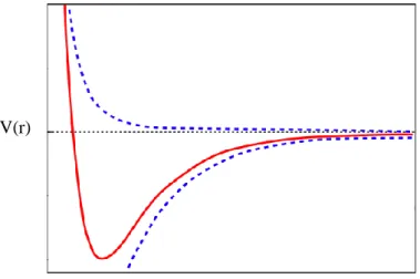
Molecules interact through space via non-bonded interactions, such as Van der Waals and electrostatic interactions, and are modeled as an inverse function of distance [3]. Several mathematical models are used to describe these interactions, namely the Lennard Jones, figure 1.1, or Buckinham potential.

The Lennard-Jones potential, figure 1.1 , is an unbounded function which is used to describe the interactions between a pair of uncharged atoms or molecules, and it has the form given in equation (16).

The 𝑟−12 is the repulsive term, and describes Pauli repulsion at small distances; while the 𝑟−6 _{term represents molecular attraction at long distances. [3-10]}

𝑈𝐿𝐽 = 4𝜀 [( 𝜎 𝑟)

12

− (𝜎_𝑟)6] (16)

The parameters sigma and epsilon have the following physical meaning: 𝜎 is the distance at which the potential is zero, and 𝜀 is the depth of the potential well Therefore, at a distance r < 𝜎 the potential should be repulsive, and the minimum of the potential is a 𝑟𝑚 = 21/6𝜎. For values of 𝑟 > 𝑟𝑚 the potential is attractive, and between rm and . As 𝑟 → ∞ the potential is attractive and decays as 𝑟−6 , which is a correct asymptote for London dispersion forces[7]. On the contrary, as 𝑟 → 0 the potential is repulsive, and decays as 𝑟12_{. In fact, this fast decay implies that molecules} cannot approximate at distances for 𝑟 < 0.9𝜎. Therefore the Lennard Jones potential may be unsuitable to model some materials. However, the repulsive term can be replaced by a functional form that smooth the decay, a so called soft core potential. However the Lennard Jones potential is suitable to model most of the interactions in many systems, and it has several advantages when compared with other types of potentials [3,4].

V(r) r Repulsive term Attractive term σ ε

Figure 1.1 Lennard Jones Potential. In shaded blue the repulsive and attractive terms are represented. The red color curve represents the curve of a Lennard Jones potential. []

14 The calculation of all these interactions is a time consuming procedure. Accordingly, for a system of N particles the time needed for evaluation of the forces is N2 _{[2]. Thus, there are}

several methods to compute long range interactions in order to reduce the time scale from N2 to N. One way is to truncate the potentials to a cutoff distance, figure 1.2, beyond which interactions are not taken into account.

However this procedure can introduce serious artifacts. There are three types of truncation: simple, shifted, and switched. In a simple truncation the potential is zero beyond for r >rc, thus the energy is not conserved [15]. The shifted and switched truncations allow a smoother

decay of the potential that gradually goes to zero at the cut off distance [3, 15]. Electrostatic interactions are given by a Coulomb potential.

Figure 1.2 This figure highlights a cut –off radius. Here is shown that molecules inside the cut radius of a reference molecule are accounted for the non bonded force calculation, in green, while the others, in blue, are not taken into account.

15

1.2.

1.2.1. Coarse Grained Models

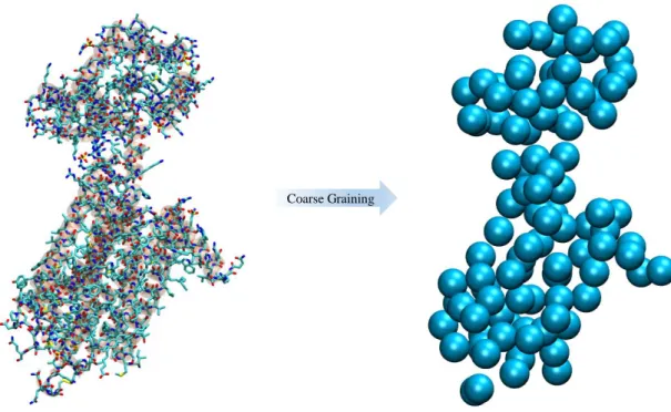
Indeed Molecular Dynamics is a powerful method to simulate large systems, however time scales beyond nanosecond are not feasible due to the high computational time and cost. Therefore modelling methods, like coarse grained, in which atoms are grouped and represented by point masses, named as beads [16]. Such reduction in the degrees of freedom, enables larger time steps, and consequently longer simulations. This is represent in figure 1.3, where is shown a basic coarse grained representation of B12 vitamin [17].

These methods are used when the time scale of the phenomena is inaccessible through full atomistic representation, as well as when global properties of a system are being studied. However it is important to remember that with the use of these methods important structural information can be lost due to the crude representation of the system [18-24].

Coarse Graining

Figure 1.3- Representation of coarse graining a protein. The right side shows a Coarse Grained representation, and at the left a Fine Grained one. This figure highlights the simplicity of a Coarse Grained model when compared to a Fine Grained one.

16

1.2.1.1. Coarse Graining by force matching

The Coarse Grained sites interact by potentials, V(R), and the configuration distribution is given by [24]:

𝑃𝑅(𝐑) ∝ 𝑒 [−V(𝐑)

𝜅𝐵𝑇] ₍₁₇₎

where R represents the Cartesian coordinates of the Coarse Grained beads. In hierarchical models, or hybrid models that combine different levels of description in one model (see section 1.2.3), the coordinates of the Coarse Grained sites are determined by mapping functions, M (𝐫) = {M₁(𝐫), M2(𝐫) … M𝑁(𝐫)}, which result from linear combination of the coordinates of the mapped Fine Grained atoms, as shown in equation (18):

M𝐼(𝐫) = ∑ 𝑐𝐼𝑖𝐫𝑖 𝑖

where r represents the Cartesian coordinates of the atomistic molecules. Notice that, a Coarse Grained model is consistent if the canonical distribution is equal to the probability distribution the atomistic one:

𝑃𝑅(𝐑) = 𝑝𝑅(𝐑) (19)

where 𝑃𝑅 is the canonical distribution of the Coarse Grained model, and 𝑝𝑅 is the distribution for sampling an atomistic configuration.

The potential for a Coarse Grained model is given by equation (20), and the force derived from that potential is expressed in equation (21):

𝑉0_{(𝑅) = −𝑘}

𝐵𝑇Ln𝑃𝑅(𝐑) + const (20)

and

F𝐼0(𝐑) = 〈f𝐼(𝑟)〉𝑅 (21)

where f𝐼(𝑟) is the atomistic force acting on site I. Notice that, the potential is a Mean Force Potential (PMF), and consequently the force is a Mean Force. However there are other ways to derive Coarse Grained force fields, and the MARTINI force field [25-26] can be given as an example.

17 Thus, the application of this technique depends on the nature of the problem. There are several approaches to coarse grain a system, such as the Go like model [27], the Elastic Network Model [28], as well as the MARTINI model [25-26], among others.

1.1.1.2.

The MARTINI model

The MARTINI force field was developed by Marrink et al, in which the main goal was to develop a force field with a wide range of applications defining as few beads as possible. The Martini force field was parameterized to fit experimental data, such as partition coefficients [25-26]. Moreover, the main concern was not to build a force field that is reproduces the structural details of the atomistic model, but to build a simple, and transferable force field. Therefore the MARTINI force field has the advantage of being highly transferable, simple, and applicable to a wide range of biochemical systems.

The MARTINI force field comprises four main interaction sites: Polar, Non Polar, Apolar, and Charged. The beads are divided into subgroups taking into account polarity, and hydrogen bonding character. This subdivision attempts to represent more accurately the chemical nature of a fine grained system. In figure 1.4 it is shown a representation of a lipid within the MARTINI scheme [25].

Here, linear molecules have four to one mapping, which means that four heavy atoms are grouped into an interaction site. However for rings, a two or three to one mapping is used, in order to maintain geometrical details. It important to note that rings can be modelled with a S type bead, for which parameters are different [26].

The bonded potentials are described by typical harmonic potentials: 𝑉𝑏𝑜𝑛𝑑(𝑅) = 1 2𝑘𝑏𝑜𝑛𝑑(𝑅 − 𝑅𝐵𝑜𝑛𝑑) 2 ₍₂₂₎ Q0 Qa Na C1

Figure 1.4 – MARTINI representation of a lipid. The different colors represent the different bead types in which the different groups of atoms are mapped.

18 where the equilibrium distance is 0.47 nm, and the force constant is 1250 kJ mol-1 _nm-2_{. In turn}

the angular potential is a cosine type potential.

𝑉𝑎𝑛𝑔𝑙𝑒(𝜃) = 1₂𝑘𝑎𝑛𝑔𝑙𝑒(cos(𝜃) − cos (𝜃0))2 (23) The angular force constant differs for aliphatic chains, and cis/trans unsatured bonds. The angular force constant for aliphatic chains of 25 kJ/mol with a corresponding equilibrium angle of 180º. In turn, the angular force constant for cis and trans unsaturated bonds is 45 kJ mol-1_{, while}

the equilibrium angles are for cis 120º, and for trans 180º. The different values allow a better fit with atomistic models [26].

Non bonded interactions are given by a 12-6 Lennard Jones potential, equation (24), where sigma represents the closest distance between two beads, while epsilon represents the interaction strength between beads.

𝑈𝐿𝐽(𝑟) = 4𝜀𝑖𝑗[( 𝜎𝑖𝑗 𝑟) 12 − (𝜎𝑖𝑗 𝑟 ) 6 ] (24)

The value of sigma is the same for almost all beads, σ=0.47 nm. However there are three exceptions namely rings where σ=0.43 nm, antifreeze particles, and for the interaction between charged and apolar beads in which σ=0.62 nm. In the same way, the epsilon value corresponds to 0.75 times the corresponding normal bead, which in practical terms means a weaker interaction. The modification of such parameters for ringlike particles enables a closer packing and avoids freezing, allowing a better reproduction of experimental densities and partition coefficients.

The interactions between beads are divided in 10 levels, in which level O is the strongest interaction while level IX is weakest interaction level. [26] Therefore, the interaction level O is used to model strong polar interactions, level II to III models volatile liquids, like ethanol, and level IV is used to model nonpolar interactions. In turn, level V to VIII describes hydrophobic repulsion between polar and nonpolar beads.

In the current work four different particles to map the solvents were used, namely a P4 type bead for water, a P2 bead for ethanol, and a SC3 and SC4 bead for toluene.

A P4 type bead corresponds to a more polar type bead, for which the level of interaction with another particle of the same type is I. Notice that, such level is used to model polar interactions and corresponds to one of the strongest interactions for which the interaction energy is 5.0 kJ/mol. In turn, the interaction of a P2 type bead with another of the same type has an interaction level of II that is a weaker interaction for which the energy is 4.5 kJ/mol.

19 The non bonded interactions in MARTINI force field are modelled by a shifted cutoff that smoothens the potential decay, for which the cutoff distance is 1.2 nm. However, the Lennard Jones Potential is shifted at 0.9 nm, while the electrostatic potential is shifted at 0.0 nm. [29]

Coarse graining has proven to be a powerful Molecular Dynamics technique to model large systems, especially when the phenomena that is being studied is not accessible via fine grained simulations. However, the loss of important structural details when using such models is a limiting factor. Multiscaling Molecular Dynamics is a technique that can be used to overcome such limitations, allowing to gather the accuracy of fine grained simulations with the speed of Coarse Grained ones.

1.2. HYBRID MOLECULAR DYNAMICS METHODS

Many biochemical processes occur in time lengths beyond the nanoscale scale, thus are not accessible through full atomistic simulations. On the other hand, the application of coarse grained methods to study these problems may not be appropriate due to the loss of important structural information. Multiscaling or Hybrid CG/FG methods combine in the same simulation both scales. Therefore, by using such techniques it becomes possible, for example, to simulate the part of interest atomistically, while the surroundings are coarse grained [30-31]. One of the main advantages of these approaches is a longer time simulation comparing to pure fine grained methods. This is so, because of the reduction in the degrees of freedom resulting from the coarse graining of the system.

In the current work Adaptive Resolution Scheme (AdResS) [32] method was used to simulate different solvents. It is relevant to note, that the Coarse Grained part is treated with the MARTINI GC model [25], while for the atomistic OPLS-AA[33], in the cases of ethanol and toluene.

1.2.3. The Adaptive Resolution Scheme – AdResS

The Adaptive Resolution Scheme allows the on-the-fly change in the degrees of freedom [34]. Therefore molecules change their resolution from fine grained to Coarse Grained, and vice-versa, according to the region of space they are in. Therefore the space is divided in three different regions: the coarse grained region, where molecules are represented by virtual sites; the transition/hybrid region, where molecules are hybrid which means that they are neither CG nor FG; and the fine grained region, in which molecules are represented fully atomistically [35]. This is explained in the figure 1.5, where the different regions that compose the AdResS method are illustrated.

20 In so doing the simulation box is divided in three different regions, where, in the center, is the higher resolution region (the atomistic layer), and in the external part, is the coarse grained region (low resolution layer). Between these two regions there lays a transition zone, also known as hybrid region [36-38]. Here molecules become gradually and smoothly coarse grained or atomistic, depending on the direction of the diffusion. In this manner if a molecule is coming from the coarse grained region towards the atomistic there is an increase in the atomistic identity, while, on the contrary, when molecules diffuse to the coarse grained region, there is a decrease in the atomistic identity.

The main idea behind AdResS is that molecules can interchange from a coarse grained region to an atomistic region by changing their degrees of freedom on the fly. Thus a molecule, that changes from an atomistic region to a coarse grained region, gradually decreases the rotational a vibrational degrees of freedom, until a final stage where only translational DOFs are left. This means that particles change gradually the level of resolution when diffusing between the different regions of space. Such change in resolution is a remarkable difference when compared to other methods of multiscaling [37]. In fact, AdResS allows a smooth transition while other types of methods do not, once the system is strictly divided into layers. Such type of partitioning becomes very useful when applied to study of polymers in solution, as well as to model chemical reactions. This is so, not only, because of the gain in computational time, but also due to combination of regions with different accuracies.

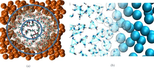
There are two different geometries that can be applied within this methodology, a spherical geometry, as shown in figure 1.6(a), and an axial geometry, as shown in figure 1.6(b) [38].

Coarse grained Hybrid Atomistic

Figure 1.5 Illustration of a simulation box within Adapative Resolution Scheme. The Coarse Grained part is shown by beads in opaque representation, while in the atomistic region it was used a full representation of the atoms. The increase in the atomistic identity is shown by beads that gradually become more transparent.

21

The distance to the explicit region is given by :

𝑥 = {

|(𝑅⃗ 𝛼− 𝑅⃗ 𝑐𝑡) ∙ 𝑒̂|

axial splitting |𝑅⃗ 𝛼− 𝑅⃗ 𝑐𝑡| spherical splitting

(25)

where 𝑅⃗ 𝑐𝑡 is the center of the atomistic layer, and 𝑅⃗ 𝛼 is the mapping point molecule α and 𝑒̂ is the unit in the splitting direction [38].

At this moment some questions appear namely: how this smooth transition is achieved, and how the overall system is affected? This transition is achieved by a weighting function which confers a different atomic identity to molecules according their position in space [39].

As stated, the system is composed by three different regions. In the coarse grained region molecules are represent through the center of mass with only translational degrees of freedom. In the fine grained region molecules are explicit, and all degrees of freedom are taken into account [32]. The hybrid region is more complex, since molecules gradually change DOFs. This smooth transition is achieved by a weighting function w, which confers to a molecule a different atomistic character. This function takes its values in the interval [0,1], where 0 corresponds to a molecule which is in the coarse grained region; and 1 is the weight of a fine grained molecule. In turn, molecules in the hybrid region have weights in ]0,1[, since they are neither atomistic nor coarse grained. Therefore the weighting function is defined as follows [40]:

(a) (b)

Figure 1.6 Schematic representation of the different geometries used in AdResS Molecular Dynamics simulations. (a) Shows a spherical geomtery. (b) Shows a slab geometry.

22 where r is the distance between the centers of mass of the molecules, and 𝑑𝑎𝑡, 𝑑ℎ𝑦 are the widths of the atomistic and hybrid layers[39].

Although other types of weighting functions could be used, the choice of cos2 _function

was made by taking into account the fact that such function should be monotonic, continuous, differentiable, and with zero slope in the Coarse Grained and atomistic frontiers, figure 1.7 [42].

As a result of the changing in resolution a molecule moving from the coarse grained region to the fine grained region (only has translational DOFs) increases degrees of freedom to a fine grained molecule with 3N-3 DOFs . The weighting function represents the basis of all this method, and the force between molecular pairs is calculated taking into account the weighing function. These physical principles were implemented in simulation packages, such as EsPreSSo, GROMACS, and Package Magic. The Espresso package was pioneer, in contrast to GROMACS in which AdResS method was recently implemented [43]. Even following the same physical principles, these simulation packages differ in some features, and consequently enable different applications.

The force resulting from the interactions between molecules is affected by the weighting function. This is so, because the resulting force arising from hybrid, Coarse Grained, and Fine Grained interactions are different[40].

𝑤(𝑟) = { 0 : 𝒓 > 𝑑𝑎𝑡+ 𝑑ℎ𝑦 𝑐𝑜𝑠2( 𝜋 2𝑑ℎ𝑦(𝑟 − 𝑑𝑎𝑡)) : 𝑑𝑎𝑡+ 𝑑ℎ𝑦 > 𝒓 > 𝑑𝑎𝑡 1 : 𝑑𝑎𝑡> 𝒓+ 𝑑ℎ𝑦 (26) 𝑤 𝑟 (𝑛𝑚) CG FG Hy 0 1

Figure 1.7 weighting function used in AdResS. As shown, this function returns 0 r values beyond 𝑑𝑎𝑡+ 𝑑ℎ𝑦, and returns 1 for r values above 𝑑𝑎𝑡. For values of r between 𝑑𝑎𝑡+ 𝑑ℎ𝑦> 𝒓 > 𝑑𝑎𝑡 the function smoothly increases, which allows the smooth increase in molecular DOFs.

23 The total intermolecular force acting between different pairs of molecules α and β is given by:

𝐹𝛼𝛽𝑇𝑜𝑡𝑎𝑙= [1 − 𝑤(𝑋𝛼) 𝑤(𝑋𝛽)]𝐹𝛼𝛽𝐶𝐺+ 𝑤(𝑋𝛼) 𝑤(𝑋𝛽) ∑𝑖𝜖𝛽∑𝑗∈𝛼𝐹𝑖𝑗𝐴𝐴 (27)

where 𝑤 is the weighting function, 𝐹_𝑖𝑗𝐴𝐴 is the sum of all atomistic interactions, 𝐹_𝛼𝛽𝐶𝐺is the effective potential between two centers of mass α and β. Thus, explicit molecules (𝑤 =1) will interact via atomistic potential, and coarse grained molecules (𝑤 =0) will interact by effective pair potential. Coarse grained and fine grained molecules will interact through the centers of mass, and the total intermolecular force is distributed to the explicit atoms of the Fine Grained molecule [39].

As stated before, the number of DOFs increases while a molecule transits from CG to AA region, in which a molecule orients in space as result of intermolecular potentials. When a molecule is entering in the Hybrid region from the Coarse Grained side, overlaps between atoms may occur, as a result of the random orientation of hybrid molecules. Therefore in order to avoid such artifacts the potential is capped, and the force resulting from these interactions cannot diverge [32]. Note that, such force capping is only present at the Coarse Grained Hybrid boundary. The force truncation is not the only possible implementation for restricting a potential at a certain value. In fact, the implementation of soft core potentials that, similarly, restrict the force at a certain value is also possible. The main difference between force capping and soft core potentials is that for SCP the potential truncation is made in function of the atomic distance.

Another particular feature of this method is that there is no Hamiltonian to define the overall energy of the system, and the system is not conservative. Moreover the total force of system is given by equation (27), and cannot be derived from a potential function [31]. This force interpolation causes artifacts in the system, such as density fluctuations along the simulation box. In practical terms this means that, the density profile is not homogenous throughout the simulation, as a consequence of a mismatch in chemical potentials of the different regions. On the contrary, molecules will have a tendency to accumulate in certain regions of space, where the chemical potentials is lower, resulting in an unrealistic density profile [49]. Therefore, in order to overcome this artifact it is necessary to derive interaction potentials for hybrid molecules that match the radial distribution function and the pressure if the atomistic region, (Iterative Boltzmann Inversion), or to apply a density correction by the use of a correction potential, which eliminates such dissimilarities, and in some cases both methods are needed.

It is relevant to note that the definition of temperature in such method is not straightforward, due to the change in the degrees of freedom on the fly. Notice that, the increase or decrease in the DOFs is made by adding or removing latent heat. Therefore, the definition of temperature in the transition region requires a special approach [41].

24 The temperature in the atomistic or coarse grained region can be defined by application of the equipartition theorem. Notice that in these regions the number of degrees of freedom is well defined. However in the transition region the number of degrees of freedom is variable [42]. A molecule passing from the coarse grained region to the atomistic region needs latent heat to reactivate rotational and vibrational degrees of freedom. In turn, a molecule that is transiting from the atomistic region to the Coarse Grained loses degrees of freedom, and consequently heat. In AdResS it is necessary to rearrange the equipartition theorem to a fractional DOFs [18], in order to calculate the temperature in transition region. [42] Hence, the kinetic energy of molecules in the hybrid region is given by:

⟨𝐾⟩𝛼 = 𝛼𝑘_𝐵𝑇

2 (28)

where ⟨𝐾⟩𝛼total average of the kinetic energy, and 𝛼 Level of resolution. The equipartition theorem generalizes to equation (28), where the kinetic energy is associated with a fractional number of degrees of freedom by a parameter α. This equation shows how latent heat can be provided or taken when a molecule is in the transition region. Notice that it is necessary to use thermostats locally coupling the particle motion, such as Dissipative Particle Dynamics Thermostats [43].

Another feature that needs a special approach is the resulting density of liquid simulations with these methods. In fact, the density inhomogenities need to be corrected in order to enable the application of these technique to the measurement of biochemical properties of a system [41].

The resulting density of a liquid simulation using AdResS is typically inhomogenous. Such an artifact is related with the fact that the effective potential arising from hybrid interactions is not the same as the Coarse Grained or the atomistic one. Moreover, the different pressures between both FG and CG region results in a drift force that causes migration of molecules to a region where the pressure is lower, and consequently in an excessive density in one of the regions. In order to reduce density inhomogenities an external potential is applied [42]. This reduces the pressure differences between Coarse and Fine Grained regions, which decreases molecular fluctuations along the simulation box. Such methodology called Thermoforce Correction is implemented in the VOTCA package, and it is an iterative procedure in which the external potential is corrected at each step [43]. The density variations are dissipated by the application of work that compensates the force drift responsible for molecular migration. The force used to compensate this artifact is given by:

𝐹𝑡ℎ(𝑥) = 𝑀𝛼

25 where 𝑝(𝑥)is the local pressure of the target density, 𝑀𝛼is the mass of a molecule α, and 𝐹𝑡ℎis the force acting on molecule α, and 𝜌0 is the target density [50]. This force is applied in the transition region, and consequently the force acting on the centers of mass of the hybrid molecules is changed by 𝐹𝑡ℎ. The actual force acting on the COM is given by:

𝐹𝛼 = ∑ 𝐹𝛽 𝛼𝛽+ 𝐹𝑡ℎ(𝑥𝛼) (30)

where 𝑥𝛼is the center of mass, 𝐹𝛼𝛽 is the resulting force between two molecules. This approach enables the combination of Coarse Grained and Atomistic system by equilibrating and reducing unphysical density profiles [50]. The pressure profile cannot be obtained directly, hence has to be taken from the equilibrium density, and an approximation to estimate the local pressure needs to be done. Given the overall constant density 𝜌0 an estimation of the local pressure is taken by:

𝑝(𝑥, 𝜌(𝑥)) ≈ 𝑝𝐴+ 1

𝜌0𝑘𝑇(𝜌0− 𝜌(𝑥)) (31)

where 𝑘𝑇 is the isothermal compressibility, 𝜌(𝑥) is the density without the application of an external force. Combining equations (29) and (30) it is possible to reach to a thermodynamic force that corrects the system density until a constant profile is achieved [50]. The force is given by equation (32), and it is an iterative procedure throughout which the density is iteratively refined until convergence to a target density:

𝐹𝑡ℎ𝑖+1(𝑥) = 𝐹𝑡ℎ𝑖 (𝑥) − 𝑀𝛼 𝜌₀2𝑘𝑇∇𝜌

𝑖_{(𝑥) (32)}

where 1

𝜌₀2𝑘𝑇 is called prefactor and represents the variation of the chemical potential, as shown in equation below:

(𝜕𝜇 𝜕𝜌)_𝑉,𝑇=

1

𝜌₀2𝑘𝑇 (33)

The thermodynamic force corrects the density profile by reducing the differences between pressures in the different regions disabling the excessive molecular migrations and, consequently, enabling a flat density profile [50]. It is important to note that, for AdResS method the compressibility in both regions should be approximately the same, because it allows a faster and easier convergence of density.

26

1.4. THE SYSTEMS UNDER STUDY

1.4.1. The bundled water model

The Bundled Water model (BW), created by Fuhrmans et al. [], and enables the simultaneous representation of water at a Coarse Grained and all atom level. Such description is required for multiscaling Molecular Dynamics simulations, such as AdResS. Here, four water molecules are connected by a so called restraining potential, figure 1.8, that restricts the movement of these molecules and confers a tetrahedral shape to the cluster.

Such clustering avoids the diffusion of water molecules too far from each other, and consequently reduces problems regarding the mapping. More precisely, within when molecules that are mapped in the same CG bead diffuse too far from each other it does not make sense to remapped them in the same bead. Thus such clustering avoids this problem.

One important characteristic of this model is that it can be used to combine the Simple Point Charge water model with the MARTINI Coarse Grained model. However this combination is not restricted to MARTINI force field, and can be combined with other Coarse Grained models that use a four to one mapping [25].

The restraining potential, that cluster 4 water molecules, is semiharmonic, and only the attractive part is considered, as shown in equation (34):

{ 1 2𝑘𝑑𝑟(𝑟𝑖𝑗− 0.3) 2 , 𝑟𝑖𝑗 > 0.3 nm 0 , 𝑟𝑖𝑗 < 0.3 nm (34)

where 𝑟𝑖𝑗 is the distance between oxygen atoms, 𝑘𝑑𝑟 is the force constant, and 0.3 nm is the distance from which the potential starts to be attractive. In order to reproduce the experimental density the force constant, as well as the repulsive C12 parameter of the Lennard-Jones potential had to be adjusted. Therefore, two bundled water models were derived. The differences between both models are the C12 term of the Lennard Jones potential, and the bundling force constants.

Figure 1.8 Representation of a Bundled Water, the bonds between the Oxygen atoms represent the restraining potential that preserves the water molecules clustered.

27 However, both models reproduce the density of SPC water. Within the several applications of such models namely, in biomolecular systems, as well as the use in AdResS Molecular Dynamics simulations. In the present work, model 1 from Fuhrmans et al. was used within AdResS. The Bundled Water model was mapped in a MARTINI bead type P4, the same which is used to represent MARTINI water.

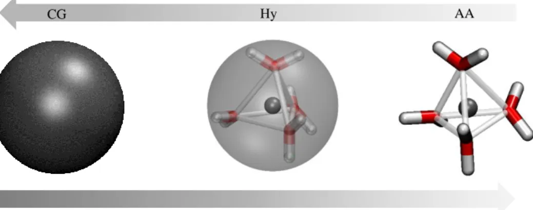
The bundled water molecules will diffuse throughout the simulation box with different levels of resolution. Hence, a full atomistic molecule will decrease in DOFs when moving towards the Coarse Grained Region, and vice versa. This is highlighted in figure 1.9, where it is demonstrated the increase or decrease of atomistic identity when a molecules are diffusing from different regions. Once in the atomistic region the four water molecules will diffuse together as result of the bundling potential.

AdResS Molecular Dynamics simulations of the Bundled Water model1 were made using GROMACS, for the spherical setup was chosen. The widths of explicit and hybrid regions were 1.0 nm. The results of this model within Adaptive Resolution Scheme simulations are shown in section 3.1.

1.4.2. Ethanol

Ethanol was chosen as a solvent due to the easier mapping compared to the bundled water. Contrary to the bundled water model, where the mapping is four to one, ethanol molecules is mapped in one to one, which, in principle, simplifies the simulations within AdResS. To describe the fine grained molecules OPLS-AA force field was used, because it is a popular choice. In turn, the Coarse Graining was made using MARTINI force field. Here, ethanol molecules are mapped into P2 type MARTINI beads, which interact with an interaction level II.

CG Hy AA

Figure 1.9 Illustration of the diffusion of a Bundled Water Cluster throughout the different regions of space within AdResS. As a cluster moves toward the coarse grained region the atomic identity decreases and the molecule is represented by a center of mass.

28

1.4.3. Toluene

The selection of toluene as a solvent was made one the basis of its challenging mapping. Here, the scenario is more complex due to the fact that toluene cannot be mapped onto one bead. Moreover the fact that in toluene molecule groups are not equivalent requires that the atoms need to be mapped in several different beads. Notice that, the representation of toluene in a single bead would give rise to a bead with a size significantly different when compared to a fine grained molecule. Moreover, in this case the geometrical details of ringlike molecules are lost resulting in a very crude representation of the Coarse Grained part. With this in mind, the toluene molecule was mapped using three beads, as represented in figure 1.10.

The Coarse Grained representation of Toluene is made by using SC3 and SC4 MARTINI type beads. As stated above S type beads were introduced in MARTINI with the purpose of modelling ringlike structures more realistically [25]. Here the interaction strength between beads is lowered 25% regarding the original value, as well as sigma that 0.04 nm smaller than for other bead types. As seen in figure 1.10, the SC3 bead includes the methyl group, and maps four heavy atoms. In turn, the other carbons are mapped into SC4 MARTINI type beads. The virtual sites are kept together by constraints, of 0.27 nm. This representation enables a better description of toluene geometry.

As fine grained toluene molecules diffuse towards the Coarse Grained region the atomistic details will be lost, and the molecule will be mapped into the three beads mentioned above.

All solvents were simulated using AdResS implementation in GROMACS package, within a spherical setup in which the size of the hybrid and explicit regions was 1.0 nm. The multibead mapping is allowed in the GROMACS package, since the bonded interactions are always present in the simulation box. This feature of GROMACS is unique, and advantageous for such type of mapping. The computation of bonded interactions in the Coarse Grained region

3 1 2 4 5 6 7 SC3 SC4 SC4

Figure 1.10 Scheme of the mapping used for the Toluene molecule. The different colors for the beads represent the different bead types that were used to map the toluene molecule.

29 allows the multibead mapping, because the centers of mass are kept together as a consequence of these interactions. In the case of the original implementation, in which bonded interactions are not calculated in the Coarse Grained region, such mapping is not possible. This is so, because the destruction of bonds in this region makes beads to move further apart from each other.

30

2. M

ETHODOLOGY

2.1. BUNDLED WATER MODEL

2.1.1. Fine Grained simulations

Molecular Dynamics simulations of 4000 bundled water molecules were carried out in a cubic box with initial dimensions of approximately 5.0 × 5.0 × 5.0 nm, at constant pressure of 1 bar and temperature of 300K. The system was equilibrated during 1 ns. For thermostatting a Berendsen thermostat with a time constant of 𝜏= 0.2 ps -1 _{was used. In turn, a Berendsen barostat}

with a time constant of 𝜏= 0.2 ps -1 _{was used. The interaction parameters were taken from}

Fuhrmans et al. The van der Waals interactions were treated with a shifted cut off of 1.4 nm, as well as the electrostatic interactions. After equilibration the final volume and density of the system were determined. This volume was applied to a constant volume simulation, which was carried out during 1 ns using the same parameters described above.

2.1.2. Coarse Grained simulations

Coarse Grained Molecular Dynamics simulation of 1000 P4 type MARTINI beads were made during 1 ns at constant volume of 125 nm3_{, corresponding to the atomistic equilibrium}

volume, and at a temperature of 300 K. The note that the value derived from the NPT fine grained simulation. As a thermostat a Berendsen with a time constant of 𝜏= 0.2 ps -1 _{was used. The}

interaction parameters were taken from the MARTINI force field. The electrostatic interactions are treated using a shifted a cut off of 1.2 nm. In turn, a shifted cut off of 1.2 nm was used for van der Walls interactions.

2.1.3. Adaptive Resolution Simulations

AdResS simulation of 4000 bundled water molecules were carried out, in a spherical step up, at a constant volume of 125 nm3_{, corresponding to the atomistic equilibrium volume,}

temperature of 300 K, and during 1ns. The radius of both explicit and hybrid layers was 1.0 nm. Here, the fine grained region was represented with GROMOS 53a6, while the for the Coarse Grained region MARTINI FF was used.

31

2.2. ETHANOL

2.2.1. Fine Grained simulations

All atom simulations of 1000 ethanol molecules were carried out a in a cubic box with initial dimensions of approximately 4.7×4.7×4.7 nm, at a constant pressure of 1 bar, and temperature of 300 K. Both Berendsen thermostat and barostat were used with a corresponding time constant of 𝜏= 0.5 ps -1_{. The interaction parameters were taken from the OPLS force field, in}

which van der Waals and electrostatic interactions are treated with a shifted cut off of 1.2 nm. The equilibrium density and volume was taken from this simulation, and posteriorly employed in a NVT simulation. Constant volume simulation was done at 300 K, and using the same parameters for the non bonded interactions.

2.2.2. Coarse Grained simulations

Coarse Grained simulations of 1000 P2 type MARTINI beads were carried out during 20 ns at constant pressure in a cubic box with initial dimensions of 4.6×4.6 × 4.6 nm, and temperature of 300K. The equilibrium volume, and density was analyzed and compared with the all atom simulation. Posteriorly constant volume simulations at 300 K and during 20 ns were done at the fine grained equilibrium volume.

2.2.3. Parameterization of the P2 type MARTINI beads

A parameterization of values of sigma and epsilon of the P2 type MARTINI beads was made in order to find the best combination that yields liquid ethanol at the pressure of 1 bar at the fine grained volume. Therefore a set Molecular Dynamics simulations were carried out during 20 ns for values of sigma and epsilon within a range of [0.31-0.45] nm, and [2.0-6.0] kJ/mol, respectively. The best combination was posteriorly applied to AdResS simulations.

2.2.4. AdResS simulations

Constant pressure AdResS simulations of 1000 ethanol molecules were carried in a cubic box with initial dimensions of 4.6×4.6×4.6 nm out at 300 K, in which the radius of both explicit and coarse grained region was 1.0 nm. In order to evaluate the influence of the width of the hybrid layer in the resulting density profile, a set of simulations was made using the following values for the radius of the hybrid region 0.5 nm, 0.7 nm, 1.0 nm.

32 The attempts to correct the density resulting from AdResS simulation was made using VOTCA package. Here a set of Molecular Dynamics simulations in which an external force is applied to correct the density mismatch was performed. At first the correction was applied to a box radius from 0.8 to 2.2 nm. However, in an attempt to correct the density mismatch in the atomistic region the correcting force was extended to a range of 0.5 to 2.2 nm.

2.3. TOLUENE

2.3.1. Fine Grained simulations

Molecular Dynamics simulations of 1000 toluene molecules in a cubic box of dimensions 5.6×5.6×5.6 nm were made during 2 ns at constant pressure of 1 bar, and temperature of 300 K. For thermostatting as for barostatting a Berendsen thermostat and barostat were chosen. The interaction parameters were taken from [46], in which van der Waals and electrostatic interactions were treated with a shifted cut off of 1.2 nm. The equilibrium density and volume were analyzed, and posteriorly the equilibrium volume was implemented to fine grained and coarse grained constant volume simulations. The constant volume simulations of 1000 toluene molecules were carried out during 2ns at a temperature of 300 K, in which the same interaction parameters were used.

2.3.2. Coarse Grained simulations

Coarse Grained Molecular Dynamics simulations of 3000 SC4/SC3 MARTINI type beads were made during 2 ns at a constant volume of nm3_{, and temperature of 300 K. The}

parameters were taken from the MARTINI force field, in which van der Walls and electrostatic interactions were treated with a shifted cut off of 1.2 nm. The final pressure was evaluated and compared with the one obtained from the fine grained simulation.

2.3.3. AdResS simulations

AdResS simulations of 1000 all atom toluene molecules were made at constant volume, and at 300 K. The radius for both explicit and hybrid layers was of 1.0 nm. In attempt to correct the resulting density a set of Molecular Dynamics simulations, in which an external correcting potential is applied, were made. The correction of the density mismatch was applied from 0.75 to 2.2 nm.

33

3. R

ESULTS

3.1. THE BUNDLED WATER MODEL

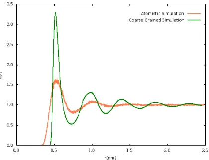
Fine grained (FG) MD simulations of 4000 Bundled Water (BW) [REF] molecules using Gromos 53a6 were carried out during 1ns, at 300 K, and at constant pressure of 1 Bar. In turn, Coarse grained (CG) MD simulations of 1000 P4 type MARTINI beads [REF] were made during 10 ns at constant pressure of 1 Bar, and at a temperature of 300 K. The density values from both FG and CG simulations were 951.33 ±0.04 kg/m3_{, and 981.69±0.07 kg/m}3_{, respectively. The fact}

that density differs 3% enables the combination of these two models in adaptive resolution simulations (AdResS2_).

The radial distribution function of COM-COM3 _{of both simulations is shown in figure}

3.1, where orange represents the atomistic rdf and green the coarse grained.

In the atomistic rdf two broad peaks are visible at 0.6 nm and 0.9 nm, respectively, that level off to g(r) = 1 for a distance beyond 1.2 nm. In turn, the CG rdf has four peaks, and the most prominent appear at 0.5 nm and 0.9 nm. When comparing both rdfs there are notable differences, not only in the number of peaks, but also in the shapes. Such that in the fine grained rdf peaks are broader, when compared to the coarse grained. Thus, the large number of peaks in the CG rdf indicates a more organized structure. Notice that, radial distribution functions of liquids, usually, comprises two main peaks at short distances, that go to g(r) =1 as the distance increases. This is

2 _{AdResS – Adaptive Resolution Scheme} 3 _{COM –Center Of Mass}

34 so, because in first solvation shell particles tend to be more organized, which gives rise to peaks at short distances. Nevertheless, as the distance increases molecular organization decreases, and so molecules have random distributions in relation to the reference particles, and consequently g(r) goes to unity. However, the type of potentials used to describe non bonded interactions, such as Lennard Jones, can introduce higher order in a system since particles cannot reach distances less than 0.9σ, and as result the system becomes over structured. This is the case in MARTINI, where beads interact by (modified) Lennard Jones potentials, and consequently are more structured when compared to the COM of fine grained models. Such is shown by the differences between AA and CG rdfs, and is the underlying reason of such dissimilarities.

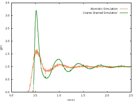
Constant volume atomistic simulations of 4000 BW molecules were made during 1 ns at 300 K, using Gromos53a6 FF. Coarse grained simulations of 1000 P4 type MARTINI beads were made during 1 ns at constant volume of 125 nm3_{, and temperature of 300K. The atomistic}

equilibrium volume was chosen for all simulations, because the final density is closer to the experimental value, which is important for solvation effects. Note that, it is possible to perform the same simulations at the coarse grained equilibrium volume. However, for cases in which the CG equilibrium volume is differs substantially from the fine grained one, would give raise in a liquid with low density.

Both COM- COM4 _{radial distribution function are shown in figure 3.2, and is similar to}

the NPT rdf. Thus, is possible to conclude that the system is well equilibrated and suitable for AdResS simulation at this volume.

4 _{COM – Center Of Mass}

Figure 3.2 Bundled water center of mass rdf of fine grained (FG), orange curve, and coarse grained (CG), green curve, simulations at constant volume.

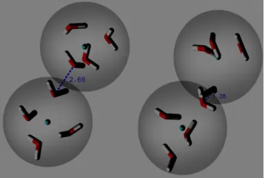
35 Adaptive Resolution simulations of 4000 bundled water molecules were made using GROMACS v4.6.0, in a spherical setup [45], at 300 K and 1 bar. The size of the explicit and hybrid regions was 1.0 nm. The simulation crashed at approximatly 10 ps due to atomic intrabead collisions when molecules were close to the frontier of the atomistic region. In fact, Oxygen atoms from the same bead (intrabead) started to overlap. This artifact is exemplified in figure 3.3, where it is possible to see that the initial distances between oxygen atoms is 2.92 Å, and decreases to 1.01 Å right before the collision.

In the oxygen- oxygen radial distribution function, figure 3.4, it is possible to see the presence of a peak at r =0.0 nm, with a corresponding g(r) of almost 2.5. This is consistent with the atomic collisions once the oxygen oxygen interatomic distance is 0.0 nm.

(a) (b)

Figure 3.3- Example of such Intrabead collisions in AdResS simulation with the bundled water model(a) Highlights the bond length ,in Å, at the beginning of the simulation, and (b) shows the bond length , in Å, before the collision.

Figure 3.4 Radial distribution function of oxygen oxygen of AdResS simulations. The inset highlights the short interatomic distances between oxygen atoms. This figure shows the short distances between oxygen atoms, and reinforces the problems that lead to crashes of such simulations.

36 Note that, molecular overlapping can occur during AdResS simulations, however it should happen near the frontiers of the hybrid-Coarse Grained region. Nevertheless, when molecules are moving towards the fine grained region the atomic identity increases and molecules orient in space avoiding each other, as result of repulsive potentials. Thus, the artifacts described above were completely unexpected.

Above all, the short oxygen distances, figure 3.4, are due to collisions inside of the beads, and are an indication of system instability. However this could be related with many factors, such as the time step, or the non bonded repulsive terms.

In order to avoid this artifact the first measure was to decrease the time step from 2fs to 1fs, which proved to be ineffective because the same problem was identified. Such interatomic distances suggested that the repulsive potentials were not being correctly taken into account. In order to add non bonded interactions between specific pairs of atoms, a pairs section was added in the topology. This option enables the definition of non bonded interaction between specific pairs of molecules, and it was used to infer if there was a problem regarding non bonded repulsive interactions. With this, a new setback occurred. This time, collisions between molecules were not intrabead but interbead, as shown in figure 3.5. In fact, when molecules were passing from the hybrid to the atomistic region water molecules from different beads started to collide.

This confirmed the previous suspicion that intrabead non bonded interactions were not being taken into account, since with the use of non bonded interactions between specific pairs of atoms intrabead collisions did not occur. However, this did not explain the interbead collisions. Notice that within AdResS molecular overlaps occur when molecules are passing from the Coarse Grained to the hybrid region. However, when hybrid molecules move towards the fine grained region they gradually increase in atomic identity, and avoid each other as consequence of repulsive interactions. This means that molecular overlaps should not occur in proximity of the

Figure 3.5 Oxygen collisions AdResS simulation. (a) Shows the initial distance between oxygen atoms of different beads. (b) Shows the distance that near the moment of simulation crash.

37 atomistic region, because molecules are almost fine grained and repulsive interactions would prevent such artifacts.

Such problems could be related either with the weighting function which was not correctly taken into account; or with an incorrect implementation of the non bonded interactions within the AdResS. Therefore, in order to discard the possibility of a source code error, this artifact was communicated to the package developers, which released a new version of the code – GROMACS v4.6.1.

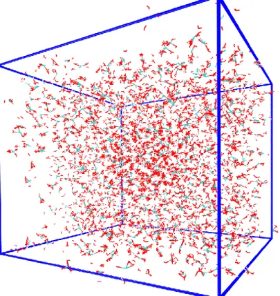
AdResS Molecular Dynamics simulations of bundled water model were made using GROMACS –v.4.6.1. Although the previous issues were not observed verified during the simulation, another phenomena occurred. As shown in figure 3.6, there is a very high density of molecules in the atomistic region, caused by an excessive molecular migration. This is also highlighted by a substantial lack of molecules in the left corner of the simulation box.

Figure 3.6 -AdResS simulation box after simulation with GROMACS version 4.6.1. In center of the simulation box it is possible so see an excess of water molecules in the center of the simulation box, which is accompanied by a substantial lack of water molecules in the left corner.

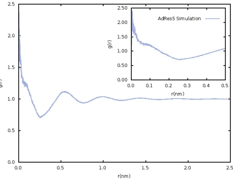
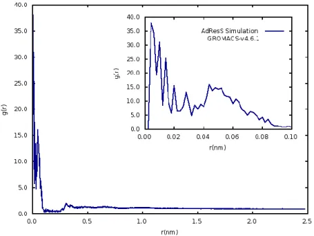
38 The radial distribution function of oxygen-oxygen, figure 3.7 , also corroborates this fact. Here is visible a very sharp peak at 0.001 nm corresponding to a g(r) of approximately 40.

The overall structure of the radial distribution function is not characteristic of any state of matter. On the contrary, it appears to be chaotic without any representative patterns of a liquid structure. Such close contacts between oxygen atoms were seen before, however this time the simulation runs until the end, while before it crashed when oxygens were overlapping. These results confirm a problem with the non bonded interactions within AdResS, since the interatomic distance suggests that repulsive potentials are not being taken into account.

In order to evaluate the non bonded interactions for hybrid molecules, bundled water simulations were carried out with a constant weight, w, throughout the box. The chosen weights values were in a range of 0.25 to 0.95. The Ox-Ox radial distribution functions, figure 3.8, are characterized by the presence of sharp peaks with a very high intensity for distances within [0.0-0.2] nm. Also, the overall rdfs do not show a structure representative of a liquid.

Figure 3.7 O-O radial distribution function of BW within AdResS, in which the short Oxygen Oxygen interatomic distances can be seen for distances comprised between 0.0 to 0.5 nm.