Combining Earth Observation and predictive modelling for multi-scale and multi-level biodiversity assessment and monitoring

D

Observation and

predictive modelling

for multi-scale and

multi-level biodiversity

assessment and

monitoring

João Francisco Fernandes Gonçalves

Tese de Doutoramento apresentada à

Faculdade de Ciências da Universidade do Porto

Departamento de Biologia

2017

D

Observation and

predictive modelling

for multi-scale and

multi-level biodiversity

assessment and

monitoring

João Francisco Fernandes Gonçalves

Plano Doutoral em Biodiversidade, Genética e Evolução

Departamento de Biologia

Faculdade de Ciências da Universidade do Porto 2017

Orientador

João P. Honrado, Professor Auxiliar e Investigador, Faculdade de Ciências Universidade do Porto

Coorientador

Caspar A. Mücher, Dr. Ir., Wageningen Environmental Research (Alterra) Wageningen University and Research

Nota Prévia

Na elaboração desta tese, e nos termos do número 2 do Artigo 4º do Regulamento Geral dos Terceiros Ciclos de Estudos Universidade do Porto e do Artigo 31º do Decreto-Lei 74/2006, de 24 de março, com a nova redação introduzida pelo Decreto-Lei 230/2009, de 14 de setembro, foi efetuado o aproveitamento total de um conjunto coerente de trabalhos de investigação já publicados, submetidos ou em fase final de preparação para publicação em revistas internacionais indexadas e com arbitragem científica, os quais integram alguns dos capítulos da presente tese. Tendo em conta que os referidos trabalhos foram realizados com a colaboração de outros autores, o candidato esclarece que, em todos eles, participou ativamente na sua conceção, na obtenção de dados e/ ou no seu processamento e análise, na discussão e interpretação dos resultados obtidos bem como na elaboração e redação dos artigos científicos aqui apresentados.

A Faculdade de Ciências da Universidade do Porto foi a instituição de origem do candidato, tendo o trabalho sido realizado sob a supervisão do orientador Prof. João Pradinho Honrado (CIBIO/InBIO – Faculdade de Ciências da Universidade do Porto), do coorientador Casper A. Mücher (Alterra – Wageningen University and Research, Holanda) e da coorientadora Isabel Pôças (LEAF/ISA – Universidade de Lisboa e CICGE – Faculdade de Ciências da Universidade do Porto). Os trabalhos foram realizados nas instalações do CIBIO/InBIO e noutras associadas aos investigadores que colaboraram no âmbito desta tese.

A elaboração desta tese de Doutoramento foi apoiada pela Fundação para a Ciência e a Tecnologia (FCT) através da bolsa de doutoramento nr.: SFRH/BD/90112/2012 do Fundo Social Europeu (FSE) e POPH-QREN (2007-2013).

Summary

(EN)

Earth Observation (EO) technologies are a powerful tool to monitor biodiversity status and change, with a vast collection of available platforms with different spatial, spectral and temporal resolutions. This variety of EO data sources is opening a wide range of opportunities for biodiversity research and for developing multi-level (from genes to landscapes), multi-scalar (from local to regional) and multi-faceted (from structure, composition up to function) monitoring systems, supported by the integration of EO data and robust modelling frameworks. Based on a comprehensive framework including those multiple biodiversity dimensions, this thesis research plan aimed to contribute to fundamental and applied research around the analysis, assessment and monitoring of biodiversity patterns and their changes. Our goal was to provide guidance and building blocks towards a cross-scale and cross-level monitoring framework supported by the integration of EO-based indicators and EO-fed models, to assist national and trans-national efforts related to the management and conservation of biodiversity.

The thesis includes three main sections: Introduction, Research papers, and General discussion and conclusions. Section I (Introduction) addresses the current challenges regarding the pressures and drivers of the global ‘biodiversity crisis’ in the Anthropocene era. A general contextualization and a broad overview of the ‘multi-dimensional’ concept of biodiversity and its impact on monitoring and assessment is presented. EO principles and data sources, as well as ecological models, are also introduced at this point. Finally, the overarching research objectives, strategy and development are described.

Section II (Research papers) includes six studies encompassing most of the scales, levels and facets that are intrinsic and relevant to biodiversity in terrestrial ecosystems. Three major topics were addressed in these studies: (i) the spatial and temporal components of functional connectivity (studies S1 to S3), (ii) habitat and ecosystem monitoring for protected area management (studies S4 and S5), and (iii) development of optimized methods for EO data processing for ecological change assessment.

In study S1 we used a comparative cross-scalar approach combining genetic tools, models, evolutionary algorithm-based optimization and EO data to investigate functional connectivity and gene flow in two Mediterranean amphibian pond-breeding species. The results clarify the effect of different landscape features on regional patterns

of population connectivity, gene flow and genetic differentiation in the two test species. Remarkable differences were found concerning the role of fine-scale patterns of vegetation cover, vegetation water content and its spatial heterogeneity in shaping patterns of regional genetic structure and gene flow for the two species. These differences in spatial heterogeneity were better portrayed by fine-scale remotely sensed spectral indices capturing land cover, vegetation and moisture in a continuous fashion. Our findings hold promising applications for addressing and evaluating functional connectivity in conservation and monitoring of vulnerable species.

In study S2, we investigated how EO-based variables related to ecosystem functioning could improve predictions and track short-term changes in habitat suitability for a vulnerable plant species. The results highlight the added value and the predictive ability of those EO-based functional variables, emphasizing their usefulness for species-level monitoring. EO time-series also contributed to clarifying the mechanisms underpinning species' temporal functional connectivity and responses to fluctuations in habitat suitability derived from multiple sources of disturbance. This holds promising applications of EO to monitor and anticipate shifts in ecosystems potentially impacting species persistence. Applications of this methodology include regional to local landscape species monitoring, management and reporting.

In study S3, we assessed the vulnerability to landscape fragmentation of reptile and amphibian species with low-dispersal abilities and facing climate and land use change. We combined Species Distribution Models (SDMs) and functional connectivity analyses to investigate the impact of fragmentation on the ability of species to track future climate change. Model projections show that environmental changes may cause severe contractions in suitable area for most test species. Moreover, connectivity analyses highlighted that potential migration corridors may be further impacted by the motorway network, making these species even more vulnerable to extinction or isolation. Contributions from this study span from methodological advances in synoptic analysis of functional connectivity up to regional and local climate change adaptation and monitoring.

Study S4 describes and tests a methodological approach for exploiting ultra-high resolution optical imagery and a digital surface model captured by an Unmanned Aerial Vehicle (UAV or ‘drone’) for fine-scale mapping of Natura 2000 priority habitats in a mountainous area under land use and rural abandonment. Our approach (based on supervised classification) obtained good overall accuracy for discriminating the target habitat types, which occur in small-scale, complex mosaics. It was also possible to

diagnose habitat quality and identify degraded patches of particular habitat types of high conservation priority. Overall, our results provide compelling indications that UAV imagery is suitable for mapping and monitoring Natura 2000 habitats, with application in protected area management and in habitat assessment and reporting on the Habitats Directive.

In study S5, we propose and evaluate an EO-based approach for measuring the performance of Protected Areas (PAs) to foster forest ecosystem stability. The approach is based on a time-series of MODIS Enhanced Vegetation Index (EVI), from which we calculated several stability metrics based on Ecosystem Functional Attributes, time-series decomposition and the non-linear Maximum Lyapunov Exponent. Then, we compared the distributions of stability metrics within and outside PAs (with similar environmental characteristics). We found a complex pattern of PA forest stability performance across the national network, both among and within PAs. Multi-model inference confirmed the pervasive negative effect of forest fires on stability, especially in mountainous PAs. Forest composition and structure also exerted a strong control over stability performance, with a positive signal related to coverage of broadleaf forests. PAs with taller and more vertically complex forest canopies, and with larger and more connected patches, were also more stable. We also found a strong positive effect of PA size, with larger parks generally holding greater stability. Potential applications of this approach are vast, spanning from PA adaptive management to disturbance control, monitoring and conservation.

In study S6, we aimed to contribute for improvement of methods in Geographic Object-based Image Analysis (GEOBIA), employed in processing (very-)high resolution EO data in ecological applications. We addressed this by optimizing the integration of two crucial steps in GEOBIA workflows: image segmentation, and classification. Genetic Algorithms were used to optimize image segmentation parameters, with synergistic benefits for both steps. A new open-source R package (SegOptim) was developed for implementing the proposed approach and dissemination. We tested this package in different settings, conditions and data sources. We found that no particular combination of an image segmentation and a classification algorithm is suited for all the tasks/objectives, suggesting an empirical verification of the “no-free-lunch theorem” for GEOBIA problems. Besides theoretical implications, this means that comparing and optimizing methods (for which SegOptim is well-tailored) is crucial to determine which ones are more suited to a particular objective. Contributions from this work span to all researchers/practitioners interested in applying GEOBIA methodologies, including ecologists, remote sensing specialists, cartographers, geographers, among others.

Finally, in Section III (General discussion and conclusions) we first summarize and link the main research contributions of each study to a broader overview around each major topic addressed in the thesis. We compare and integrate the three major approaches applied in this thesis for biodiversity monitoring and change assessment: detection, modelling, and combined. We discuss their advantages and shortcomings and provide guidelines to adopt each approach depending on the nature and objectives of global, continental (Europe) and national monitoring initiatives. We also provide a general summary of the impact and potential application of the research developed as well as possible paths to improve it. We close with a set of overarching remarks and an outlook focused on broad ‘lessons learned’, advances in the state of knowledge and methods, and a set of recommendations on operational challenges towards adopting a more “EO-based biodiversity monitoring” paradigm. Together with robust modelling frameworks, the plethora of EO data sources can (and already is) advancing the scientific knowledge regarding the causes underlying accelerated changes in biodiversity. Throughout this thesis, we supported this notion through a series of research papers that individually constitute building blocks to develop an EO-supported monitoring system. In its essence, that system could respond to the demands of national and international efforts aimed to track and halt biodiversity loss, by supporting meaningful sets of indicators to evaluate the implementation of conservation programs and policy instruments.

Resumo

(PT)

As tecnologias de Observação Terrestre (OT) constituem uma poderosa ferramenta para monitorizar o estado e as alterações da biodiversidade, com uma vasta coleção de plataformas disponíveis com diferentes resoluções espaciais, espectrais e temporais. Esta variedade de fontes de dados de OT significa que é possível desenvolver sistemas de monitorização multinível (dos genes às paisagens), multi-escalares (local até global) e multifacetados (estrutura, composição e função) suportados pela integração de dados de OT e abordagens de modelação robustas. Com base numa moldura abrangente, que inclui as múltiplas dimensões da biodiversidade, o plano de investigação desta tese teve como objetivo contribuir para a investigação fundamental e aplicada em torno da análise, avaliação e monitorização dos padrões biodiversidade e da sua alteração. O objetivo foi providenciar linhas de orientação e os elementos constituintes para desenvolver molduras de monitorização cruzando diversas escalas e níveis e suportados pela integração de indicadores e modelos alimentados por dados de OT, e tendo como objetivo assistir os esforços nacionais e transnacionais relacionados com a gestão e conservação da biodiversidade.

A tese inclui três secções: Introdução, Artigos de investigação e Discussão e conclusões gerais. A Secção I (Introdução) aborda os atuais desafios relacionados com as pressões e os fatores de alteração da ‘crise global da biodiversidade’ no Antropoceno. Uma contextualização e uma visão panorâmica geral do conceito ‘multidimensional’ de biodiversidade e o impacto deste para a monitorização e avaliação é apresentado. Os princípios fundamentais e as fontes de dados de OT, assim como, os modelos ecológicos, são também introduzidos neste ponto. Para finalizar, são descritos os objetivos gerais de investigação, a estratégia e o seu desenvolvimento.

A Secção II (Artigos de investigação) inclui seis estudos que abarcam a maioria das escalas, níveis e facetas que são intrínsecas e relevantes para a biodiversidade nos ecossistemas terrestres. Três grandes tópicos são abordados nestes estudos: (i) as componentes espacial e temporal da conectividade funcional ao nível da espécie (estudos S1 a S3), (ii) a monitorização de habitats e ecossistemas para a gestão de áreas protegidas (estudos S4 e S5), e (iii) o desenvolvimento de métodos optimizados para a o processamento de dados de OT com aplicações na avaliação de alterações ecológicas.

No estudo S1 utilizámos uma abordagem trans-escalar combinando ferramentas genéticas, modelos, otimização baseada em algoritmos evolutivos e dados de OT para investigar a conectividade funcional e o fluxo genético em duas espécies Mediterrânicas de anfíbios que se reproduzem em charcos. Os resultados obtidos clarificam o efeito de diferentes estruturas da paisagem nos padrões regionais de conectividade populacional, fluxo genético e diferenciação genética nas duas espécies. Notáveis diferenças foram encontradas relativamente ao papel de aspetos finos dos padrões de coberto da vegetação, quantidade de água na vegetação e da heterogeneidade espacial destes nos padrões regionais da estrutura genética e fluxo genético para as duas espécies. As variações na heterogeneidade espacial foram melhor capturadas pela escala-fina dos índices espectrais derivados de deteção remota, capazes de capturar de forma contínua os padrões de coberto do solo, vegetação e humidade. Estes contributos evidenciam aplicações promissoras para abordar e avaliar a conectividade funcional na conservação e monitorização de espécies vulneráveis.

No estudo S2, investigámos o potencial de variáveis baseadas em OT relacionadas com o funcionamento dos ecossistemas para melhorar as previsões e detetar as alterações de curto-prazo na adequabilidade do habitat para espécies vulneráveis de plantas. Os resultados obtidos evidenciam as mais-valias e a capacidade preditiva das variáveis funcionais de OT, enfatizando a relevância destas para a monitorização ao nível da espécie. As séries-temporais de OT também contribuíram para clarificar os mecanismos subjacentes à componente temporal da conectividade funcional e a resposta a flutuações na adequabilidade do habitat derivadas de múltiplas fontes de perturbação. Estes resultados mostram aplicações relevantes da OT para monitorizar e antecipar alterações nos ecossistemas com potenciais impactos na persistência das espécies. As aplicações desta metodologia incluem a monitorização, gestão e o relato desde a escala local da paisagem até à regional.

No estudo S3, avaliámos a vulnerabilidade à fragmentação da paisagem de espécies de répteis e anfíbios com baixa capacidade dispersão e que atualmente enfrentam alterações climáticas e de uso do solo. Modelos de Distribuição de Espécies (SDMs) e análises de conectividade funcional foram combinados para investigar o impacto da fragmentação da paisagem na capacidade das espécies acompanharem futuras alterações do clima. As projeções dos modelos mostram que as alterações ambientais irão causar contrações severas na área adequada para a maioria das espécies testadas. Adicionalmente, as análises de conectividade mostram que os potenciais corredores de migração poderão ser adicionalmente impactados pela rede

de autoestradas, tornando estas espécies ainda mais vulneráveis à extinção ou isolamento. Os contributos deste estudo estendem-se desde avanços metodológicos na análise sinóptica da conectividade funcional até à adaptação e monitorização regional e local às alterações climáticas.

O estudo S4 descreve e avalia uma abordagem metodológica para explorar imagens óticas de resolução ultra-elevada e um modelo digital da superfície capturados por um Veículo Aéreo Não Tripulado (VANT, vulgo ‘drone’) para o mapeamento a fina-escala de habitats prioritários em contexto de áreas de montanha abrangidas na Rede Natura 2000, e submetidas a processos de abandono rural e de uso do solo. A abordagem (baseada em classificação supervisionada) obteve boa exatidão geral para discriminar os tipos de habitat alvo, que ocorrem em mosaicos complexos e escalarmente finos. Foi também possível diagnosticar a qualidade do habitat e identificar parcelas degradadas de tipos de habitat particulares de elevada prioridade para a conservação. Em termos gerais, os resultados providenciam uma convincente indicação que as imagens de UAV são adequadas para o mapeamento e monitorização de habitats Natura 2000, com aplicações na gestão de áreas protegidas e na avaliação do estado de habitats para efeitos de relato da Diretiva Habitats.

No estudo S5, foi proposta e avaliada uma abordagem baseada em OT para medir a performance de Áreas Protegidas (APs) para promover a estabilidade dos ecossistemas florestais. A abordagem é baseada numa série temporal da plataforma MODIS e do Índice de Vegetação Melhorado (IVM), a partir do qual foram calculadas várias métricas de estabilidade baseadas em Atributos Funcionais dos Ecossistemas, decomposição de séries temporais e em análise não-linear através do Expoente Máximo de Lyapunov. Em sequência, comparámos a distribuição dos indicadores de estabilidade calculados dentro e fora de APs (com base em área ambientalmente similares). Em termos gerais, encontramos um padrão complexo de estabilidade florestal ao longo da rede nacional de APs, tanto entre e dentro destas. Técnicas estatísticas de Inferência multi-modelo permitiram confirmar o efeito negativo generalizado que os fogos florestais exercem sobre a estabilidade florestal, especialmente em APs de montanha. A composição e estrutura da floresta também exerceram um elevado controlo sobre a performance da estabilidade, com um sinal positivo relacionado com a cobertura de floresta de folhosas. Adicionalmente, APs com dosséis florestais mais elevados e complexos, e com parcelas mais amplas e mais conectadas foram também consideradas mais estáveis. Também encontrámos um forte efeito positivo do tamanho da AP, com parques de maiores dimensões genericamente mais estáveis. As aplicações potenciais desta abordagem são vastas, compreendendo

desde a gestão adaptativa de APs ao controlo de fontes de perturbação, monitorização e conservação.

No estudo S6, tivemos como objetivo contribuir para a melhoria dos métodos de Análise Geográfica de Imagens Baseada em Objetos (GEOBIA), aplicada no processamento de dados de OT de (muito-)alta resolução para aplicações ecológicas. Abordamos este desafio através da otimização integrada de dois processos cruciais em fluxos de trabalho em GEOBIA: a segmentação de imagem e a classificação. Algoritmos Genéticos foram utilizados para otimizar os parâmetros da segmentação de imagem, com impactos sinergísticos em ambos os processos. Um novo pacote R open-source (denominado SegOptim) foi desenvolvido implementando a abordagem preconizada e para efeitos de disseminação. Este pacote foi testado em diferentes parametrizações, condições e com diferentes fontes de dados. Os resultados dos testes indicam que nenhuma combinação particular de um algoritmo de segmentação e classificação é adequada para todas as tarefas/objetivos, sugerindo uma verificação empírica do

“no-free-lunch theorem” para problemas de GEOBIA. Para além das implicações teóricas,

isto significa que comparar e otimizar métodos (objectivos para os quais o pacote

SegOptim é perfeitamente adequado) é crucial para determinar quais são os algoritmos

mais adequados para um objetivo particular. As contribuições deste trabalho estendem-se a todos os investigadores/técnicos interessados em aplicar metodologias de GEOBIA, incluindo ecólogos, especialistas em deteção remota, cartógrafos, geógrafos, entre outros.

Para finalizar, na Secção III (Discussão geral e conclusões) começamos por sumarizar e ligar os principais contributos de investigação de cada estudo a uma panorâmica mais geral em torno de cada tópico abordado na tese. Para este efeito, comparamos e integramos as três abordagens mais significativas aplicadas no desenvolvimento da tese aplicadas à monitorização da biodiversidade e avaliação de alterações: deteção, modelação e combinadas. Discutimos as vantagens e desvantagens e evidenciamos linhas orientadores para adotar cada uma destas abordagens em função da natureza e dos objetivos de iniciativas de monitorização globais, continentais (Europeias) e nacionais. Providenciámos também um sumário geral do impacto e das potenciais aplicações da investigação desenvolvida assim como possíveis caminhos para a sua melhoria. Fechamos com um conjunto de comentários abrangentes e um outlook focado em ‘lições aprendidas’, avanços no estado do conhecimento e métodos, e num conjunto de recomendações sobre desafios operacionais em direção à adoção de um paradigma de monitorização da biodiversidade

mais suportado por dados de OT. Em conjunto com abordagens de modelação robustas, a diversidade de fontes de dados de OT pode (e já está) a avançar o conhecimento científico em relação às causas da acelerada perda de biodiversidade. Ao longo desta tese, suportamos esta noção através de uma série de trabalhos de investigação que individualmente constituem os blocos elementares para desenvolver um sistema de monitorização suportado por OT. Na sua essência, um sistema destes poderá corresponder às exigências dos esforços nacionais e internacionais direcionados para deter a perda da biodiversidade, através do suporte à obtenção de conjuntos de indicadores para avaliar a implementação de programas de conservação e instrumentos políticos.

Index

List of figures ... 20

List of tables ... 24

List of abbreviations ... 27

SECTION I. Introduction ... 31

CHAPTER 1 - Ecological change: from theory to assessment ... 33

1.1. Ecological change across scales: drivers, pressures, tipping-points

and responses ... 33

1.2. Scales, levels and ‘facets’ of biodiversity: implications for assessment

and monitoring ... 38

References ... 42

CHAPTER 2 - Methods and tools for ecological change assessment ... 45

2.1. Earth observation systems for assessing and monitoring ecological

change ... 45

2.1.1. Earth observation: principles, platforms and data ... 45

2.1.2. Applications on EO data in biodiversity science ... 51

2.2. Modelling tools for assessing change drivers and forecasting ... 55

2.2.1. Species Distribution Models (SDMs) ... 55

2.2.2. Ecological niche theory and SDM assumptions ... 57

2.2.3. Workflow and applications of SDMs ... 61

References ... 64

CHAPTER 3 - Research objectives and thesis structure ... 73

3.1. Research objectives ... 73

3.2. Research development and thesis structure... 75

SECTION II. Research papers ... 81

Sub-section II.1. Gene level – Combining genetic and Earth Observation data

for assessing gene flow and functional connectivity ... 83

Chapter 4 - Comparative landscape genetics of pond-breeding amphibians

in Mediterranean temporal wetlands: the positive role of structural

heterogeneity in promoting gene flow ... 83

DISCLAIMER ... 83

4.1. Introduction ... 85

4.2. Methods ... 87

4.3. Results... 92

4.4. Discussion ... 99

References ... 103

Sub-section II.2. Species level – Model-based assessment of habitat

suitability dynamics and vulnerability to global change ... 109

Chapter 5 - Exploring the spatiotemporal dynamics of habitat suitability to

improve conservation management of a vulnerable plant species ... 109

DISCLAIMER ... 109

ABSTRACT ... 110

5.1. Introduction ... 111

5.2. Methods ... 113

5.3. Results... 120

5.4. Discussion ... 128

References ... 133

Chapter 6 - A model-based framework for assessing the vulnerability of low

dispersal vertebrates to landscape fragmentation under environmental

change ... 139

DISCLAIMER ... 139

ABSTRACT ... 140

6.1. Introduction ... 141

6.2. Methods ... 143

6.3. Results... 150

6.4. Discussion ... 157

References ... 162

Sub-section II.3. Habitat and ecosystem levels – Exploring Earth Observation

data to assess extent, condition and stability ... 169

Chapter 7 – Evaluating an unmanned aerial vehicle-based approach for

assessing habitat extent and condition in fine-scale early successional

mountain mosaics ... 169

DISCLAIMER ... 169

ABSTRACT ... 170

7.1. Introduction ... 171

7.2. Methods ... 173

7.3. Results... 180

7.4. Discussion ... 185

References ... 190

Chapter 8 – Assessing the effectiveness of Protected Areas in promoting

forest stability – a methodological approach based on satellite time-series

data and multi-model inference ... 195

DISCLAIMER ... 195

ABSTRACT ... 196

8.1. Introduction ... 197

8.2. Methods ... 201

8.3. Results... 214

8.4. Discussion ... 223

References ... 229

Sub-section II.4. Developing novel tools for Geographic Object-based Image

Analysis (GEOBIA) of high-spatial resolution EO imagery for ecological status

and change assessment ... 235

Chapter 9 – SegOptim – a R package for optimizing segmentation

parameters with genetic algorithms for supervised image classification .. 235

DISCLAIMER ... 235

ABSTRACT ... 236

9.1. Introduction ... 238

9.2. Methods ... 242

9.3. Results... 255

9.4. Discussion ... 258

References ... 262

SECTION III. General discussion and conclusions ... 267

CHAPTER 10 – Combining EO and predictive models to improve the

monitoring of biodiversity and ecological change ... 269

10.1. Species-level monitoring in Anthropocene landscapes: a focus on

functional connectivity ... 270

10.2. Habitat and ecosystem monitoring for effective management of

protected area networks ... 274

10.3. Improving GEOBIA methods for assessment of biodiversity and

ecological change ... 277

10.4. Earth Observation detection and ecological modelling – combining

approaches for improved biodiversity monitoring and assessment ... 279

CHAPTER 11 - Conclusions and outlook ... 287

11.1. Summary of contributions and future developments ... 287

11.2. Final remarks and outlook ... 294

SECTION IV. Appendices ... 305

Appendix I | Chapter 4 - Comparative landscape genetics of pond-breeding

amphibians in Mediterranean temporal wetlands: the positive role of

structural heterogeneity in promoting gene flow ... 305

Appendix II | Chapter 5 - Exploring the spatiotemporal dynamics of habitat

suitability to improve conservation management of a vulnerable plant

species ... 323

Appendix S1 – Description of the study area ... 323 Appendix S2 – Preliminary Maxent model used for sampling design ... 324 Appendix S3 – Competing hypotheses definition, justification and support . 327 Appendix S4 – Correlation matrix for predictor variables used in model fitting ... 330 Appendix S5 – Model diagnostics ... 331 Appendix S6 – Modified Corine Land Cover (CLC): methodological notes .. 332 Appendix S7 – Species response curves for predictors ... 337 References ... 344

Appendix III | Chapter 6 - A model-based framework for assessing the

vulnerability of low dispersal vertebrates to landscape fragmentation under

environmental change... 347

Appendix S1 – Study-area description, species occurrence points and

description of the test species ... 347 Appendix S2 – Results for the spatial filtering routine applied to occurrence records ... 350 Appendix S3 – List of available GCMs from WorldClim ... 351 Appendix S4 – Land-use categories used in DynaCLUE 2050 land-use

change projections for Europe based on Corine Land Cover ... 352 Appendix S5 – Evaluation of species distribution dynamics and connectivity analyses (full methodological description) ... 353 Appendix S6 – Pearson correlation matrix for continuous predictor variables ... 357 Appendix S7 – Habitat suitability, stable habitat patches and landscape

resistance by test species and scenario ... 358 Appendix S8 – Importance of predictor variables by species and modelling technique ... 362 Appendix S9 – Habitat suitability dynamics under projections of climate and land-use change ... 364 Appendix S10 – Connectivity metrics: summary statistics ... 365 References ... 367

Appendix IV | Chapter 7 – Evaluating an unmanned aerial vehicle-based

approach for assessing habitat extent and condition in fine-scale early

successional mountain mosaics ... 369

Appendix S1 – Test-site photographs recorded during in-field campaigns .. 369

Appendix S2 – Spectral sensitivity data for Canon cameras ... 372

Appendix S3 – Features used for supervised image classification ... 377

Appendix S4 – Preliminary cross-validation results ... 381

Appendix S5 – Overall classification performance measures ... 384

Appendix S6 – References used for comparing producer and user accuracy values ... 386

Appendix S7 – Confusion matrix calculated from validation/test set 1 ... 389

References ... 390

Appendix V | Chapter 8 – Assessing the effectiveness of Protected Areas to

ensure the stability of forests – a methodological approach employing

MODIS EVI time-series data ... 393

Appendix S1 – List of selected Protected-areas in mainland Portugal... 393

Appendix S2 – Demographic changes in selected protected areas ... 396

Appendix S3 – Description of common species in Corine Land cover forest classes ... 398

Appendix S4 – Details of smoothing algorithms ... 399

References ... 399

Appendix S5 – Search buffer distances by protected area ... 401

Appendix S7 – Area covered by different forest species according to 1995 forest inventory by PA and NPA ... 404

Appendix VI | Chapter 9 – SegOptim – a R package for optimizing image

segmentation parameters with evolutionary algorithms in the context of

supervised classification ... 405

Appendix S1 – List of reviewed papers in the context of OBIA and supervised classification ... 405

Appendix S2 – Ranges of image segmentation parameters by test site ... 411

Appendix S3 – List of land cover/use classes for multi-class test sites ... 412

Appendix S4 – Confusion matrices for multi-class tests ... 413 Appendix S5 – Full list of optimized parameters by test site and algorithm . 416

List of figures

(Note: figure numbering starts by the chapter numeral followed by figure numbers within that chapter)

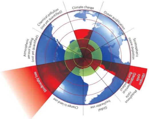
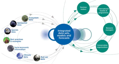
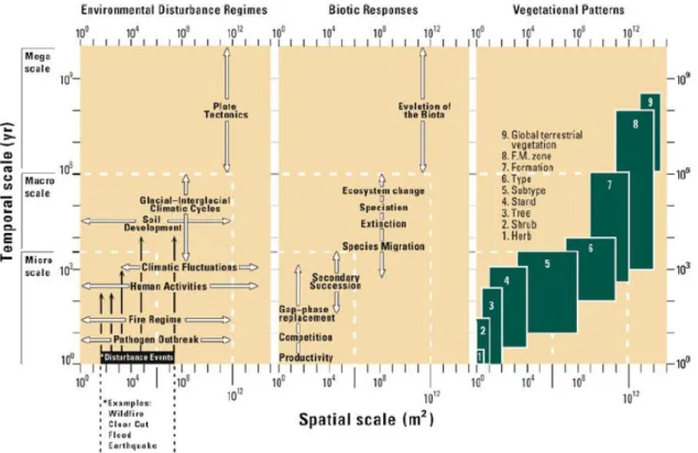
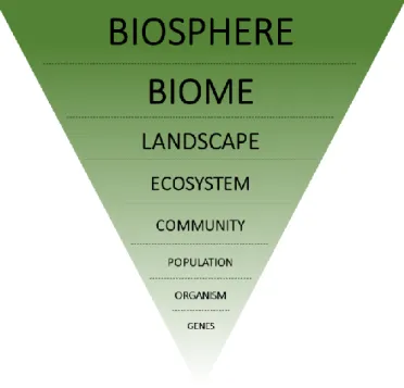
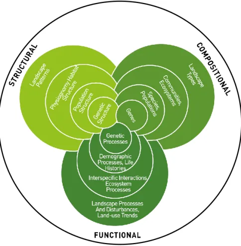
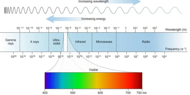
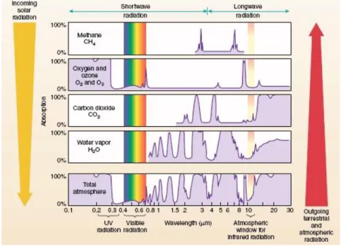
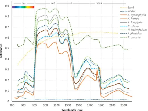
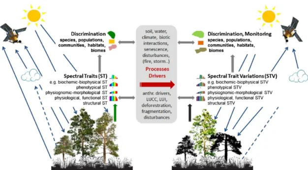
Figure 1 - 1 – A representation of the proposed safe operating space for nine planetary systems (in green colour). The red wedges represent an estimate of the current position for each variable. The boundaries in three of these systems (rate of biodiversity loss, climate change and human interference with the nitrogen cycle), have already been exceeded. (reproduced from (Rockstrom et al. 2009)) ... 34 Figure 1 - 2 – Schematic representation of safe operating space with dynamic and interacting pressures at local scale (land use change, fragmentation, species introductions, etc.) with global scale stressors (related with climate change; source: (Scheffer et al. 2015)) ... 35 Figure 1 - 3 – GEO BON – The Group on Earth Observations Biodiversity Observation Network (source GEO BON, URL: http://geobon.org/about/vision-goals).). ... 37 Figure 1 - 4 – Space-time hierarchy diagram proposed by (Delcourt et al. 1982). Environmental disturbances regimes, biotic responses and vegetational patterns are shown in the context of space-time domains. The scale for each pattern or process reflects the spatiotemporal scale required to observe or analyse it. For vegetation patterns, the temporal scale represents the time needed to record their dynamics (reproduced from: (Turner and Gardner 2015)). ... 38 Figure 1 - 5 – Eight levels of biological and ecological organization with increasing degree of complexity and interactions from bottom to top (based on: (Solomon et al. 2008) and (Allen and Hoekstra 1990)). ... 39 Figure 1 - 6 – Compositional, structural and functional biodiversity shown as interconnected spheres along multiple levels of organization. (source: Noss (1990) and redrawn in Werner and Gallo-Orsi (2016)) ... 41 Figure 2 - 1 – The electromagnetic spectrum (source: https://sites.google.com/site/chempendix/em-spectrum; © Sapling Learning) ... 46 Figure 2 - 2 – Atmospheric absorption occurring along the EM spectrum (Source: CIMSS, URL: https://cimss.ssec.wisc.edu/sage/meteorology/lesson1/AtmAbsorbtion.htm) ... 48 Figure 2 - 3 – Reflectance profiles extracted from a hyperspectral sensor showing spectral differences between alien/invasive plant species of the Acacia genus (solid lines; Acacia cyanophylla, A. karroo and A.

longifolia) and native species (dashed lines; Corema album, Halimium halimifolium, Juniperus phoenica and Pinus pinaster). Adapted and data compiled from Bradley, 2014; Lehmann et al., 2015; Mureriwa et al.,

2016. Electromagnetic spectrum ranges: Vis – Visible (390 – 700nm); NIR – Near Infrared (700-1300nm); SWIR – Short-wave Infrared (1300 – 3000nm). ... 49 Figure 2 - 4 – (a) Spectral traits (ST) for quantifying biodiversity by EO techniques (source: simplified from original Lausch et al. (2016))... 52 Figure 2 - 5 - Quantification of spectral traits and their interactions with drivers and processes to discriminate and monitor plant species, populations, habitats, communities and biomes using EO (source Lausch et al. (2016)). ... 53 Figure 2 - 6 – A simplified scheme of a SDM input and output. ... 56 Figure 2 - 7 – (a) BAM diagram representing a species niche showing the effects of biotic (B), abiotic (A) and mobility (M) aspects [adapted from: Peterson et al. (2015)]; (b) representation of the ecological niche in a two-dimensional environmental space and its relationship to species’ distribution in the geographical space (c,d). The grey area represents the Grinnellian fundamental niche (the cross sign indicates the niche optimum). Outside the niche envelope (bold line), growth is negative, decreasing until it reaches the lethal envelope (bold dashed line), beyond which the species cannot survive. The isolines, or envelopes, link all points of equal species per capita growth rate, r. (c) and (d) represent a spatial realization of the Grinnellian niche – or the ‘potential’ available habitat. A’ (green areas) – represent occupied habitat with suitable A, B, and, M conditions i.e., Hutchinson’s realized niche; B’ (red area) – representation of suitable but unoccupied

habitat due to inaccessible conditions and/or biotic constraints; A’’ and B’’ represented idealized predictions of a SDM with situations of correct, over- and under-prediction of the fundamental and/or realized niches where A’’ areas (blue) have an ‘admissible’ extrapolation contrary to, B’’ (yellow) showing a strong over-prediction of the realized niche but admissible over-prediction of the fundamental niche (for example, due to high environmental similarity with suitable locations sampled). Points show an idealized random sampling over the geographic area: black points are sample absence locations whereas green points are presence locations [adapted from Hirzel and Le Lay (2008)]... 59 Figure 2 - 8 – Typical Species Distribution Modelling workflow... 63

Figure 3 - 1 – Cross-scale and cross-level complementarity between the six research studies conducted during this PhD. Here we do not address the ‘conventional’ levels of biotic organization (Figure 1 - 5; (Allen and Hoekstra 1990)) although the obvious overlap (exceptions to ‘species’ which relates to population level; or ‘habitat’ relating broadly to the community level). Instead, we prefer to address more directly to levels at which we analysed biodiversity status and change. ... 77

Figure 4 - 1 – Sampling locations for the two study species: P. cultripes (A) and P. waltl (B). Codes as in Table 4 - 1. Results of the optimal number of clusters for each species according to BAPS are also shown. ... 94 Figure 4 - 2 – Transformations applied to each variable (included in the most frequently selected models) to generate resistance surfaces for species P. cultripes (left-side) and P. waltl (right-side). Each curve represents a different transform parameterization optimized for DEST (black color), FST (dark-grey) and G’’ST

(light-grey). Original values are represented in the x-axis (including the full range of the variable) while transformed (resistance) values are shown in the y-axis and should be interpreted in relative fashion between variables. The dashed line shows the minimum resistance for the original values of each variable. The boxplot on top shows the distribution of the original untransformed variable (boxes are the ... 97 Figure 4 - 3 – Optimized resistance surfaces for Pelobates cultripes (left-side) and Pleurodeles waltl

(right-side) based on the most frequently selected variables and considering FST genetic distances. For each

species, on the left are maps showing the original continuous values for each variable; on the right, the resistance surface generated through optimization. Points represent sampling localities. ... 98

Figure 5 - 1 – Main features of the study-area (a) and its location in mainland Portugal (b) and in Europe (c). ... 114 Figure 5 - 2 – Flowchart representing model development to evaluate the spatiotemporal dynamics of habitat suitability and to address the added-value of multi-temporal data. ... 119 Figure 5 - 3 – (a) Number of suitable habitat predictions between 2001 and 2010 for each grid unit. Burned area is displayed in proportional circles for enabling the comparison of suitable areas against fire-prone locations; (b, c) study-area broader geographical context. ... 123 Figure 5 - 4 – Plot representing the inter-annual variation in total number of suitable areas predicted (black line), along with auxiliary data related to the total amount of burned area in the study-site (in hectares; orange line) and, the variation in total annual precipitation (blue line) showing three years with severe drought conditions: 2004, 2005 and 2007. ... 124 Figure 5 - 5 – Biplots displaying the association between anomalies (annual value minus the median for the whole studied period 2001-2010) in maximum value of the growing season (left column) or Actual Evapotranspiration (right column) and anomalies in total precipitation from the previous year (identified as lag+1yr ; first row) and average minimum temperature of the coldest month (second row) which show the effect of inter-annual variations in climatic conditions in remotely sensed indicators. Values for RS variables represent the anomaly in each year (from 2001-2010) in the median across the study-area, and considering only sites predicted as suitable at least one time in 2001-2010. Rsq – coefficient of determination for the regression line; Pearson cor. – Pearson correlation between variables. ... 125 Figure 5 - 6 – Boxplots showing the effect of motorways (constructed during 2002-2006; left-side of the panel) and wildfires (right-side) on the temporal variation of predictor variables: Seasonal Amplitude (AMPLT), Maximum Value of the growing season (MAXVL) and Actual Evapotranspiration (EVPTR) for the 2001-2010 period. Plotted locations only include areas that were at least one time predicted as suitable by the averaged model. Grey boxes represent affected areas (by motorways or wildfires) while white boxes represent control/unaffected areas by both types of disturbances. Outliers were represented as circles, i.e., values lying outside the box 1.5 times the inter-quartile range. ... 126 Figure 5 - 7 – Biplots showing the association between the number of suitable areas predicted per year (one point by year between 2001-2010) and anomalies (calculated as the annual value minus the median for the whole studied period 2001-2010) in the maximum value of the growing season (left), seasonal amplitude (center) and actual evapotranspiration (right). Values for RS variables represent the anomaly in each year (from 2001-2010) in the median across the study-area, and considering only sites predicted as suitable at least one time in 2001-2010. Rsq – coefficient of determination for the regression line; Pearson cor. – Pearson correlation between variables. ... 127

Figure 6 - 1 – Schematic representation of the methodological approach developed. ... 143 Figure 6 - 2 – Barplot displaying variable importance by species and averaged across all pseudo-absence sets, evaluation rounds and modelling algorithms. Error bars represent the standard-errors across modelling techniques. Species are Anguis fragilis (ANGFR), Lacerta schreiberi (LACSH), Chioglossa lusitanica (CHALU) and Epidalea calamita (EPCAL). ... 151

Figure 6 - 3 – Boxplot of the Mean Functional Distance index by species and scenario. The yy-axis was log transformed and outliers, i.e., values 2 times the inter-quartile range outside the box, were represented as points. LES – low-emissions scenario (blue boxes); HES – high-emissions scenario (red boxes). ... 152 Figure 6 - 4 – Map representation of species distribution dynamics (a,d,g,j), connectivity between “lost” (source areas) and “kept” (target areas) using the Mean Functional Distance index (MFD, k=5; b,e,h,k), and the zonation of important areas for connectivity using the SPsum index (c,i,f,l) for each reptile species (A.

fragilis, L. schreiberi) and scenario (low-emissions scenario and high-emissions scenario) ... 154

Figure 6 - 5 – Map representation of species distribution dynamics (a,d,g,j), connectivity between “lost” (source areas) and “kept” (target areas) using the Mean Functional Distance index (MFD, k=5; b,e,h,k), and the zonation of important areas for connectivity using the SPsum index (c,i,f,l) for each amphibian species (C. lusitanica, E. calamita) and scenario (low-emissions scenario and high-emissions scenario). ... 155 Figure 6 - 6 – Boxplot showing the distributions of SPsum values for all areas important for maintaining connectivity (i.e. with 𝑆𝑃𝑠𝑢𝑚 ≥; blue boxes) and those areas intersected by motorways (red boxes) across species and scenarios (LES – low-emissions scenario and HES – high-emissions scenario). The y-axis was log-transformed, and, outliers, i.e., values lying outside the box 2 times the inter-quartile range were represented as points. ... 156

Figure 7 - 1 – Study-area location in the Iberian Peninsula and the NW region of Portugal. The test-site is fully included in the Natura 2000 “Serra de Arga” Site of Community Importance. ... 173 Figure 7 - 2 – The focal habitats as captured by the UAV platform. (a) wet heath, habitat type 4020*, in dense/large shrub formations in concave/wet areas; (b) habitat 4020* around a small pond; (c) continuous, species-rich Nardus grasslands, habitat type 6230*, with low shrub density; (d) 6230* habitat with bare soil, highlighting poor habitat condition; (e) dry heath, habitat type 4030, in mosaic with bare rock/soil areas; (f) heath (4030) encroachment on Nardus grassland denoting degradation due to decreased grazing pressure. ... 175 Figure 7 - 3 – Overview of the methodological approach tested. The scheme uses dashed boxes to denote processes (bold lettering signals important processing steps), grey boxes denote specific or detailed aspects for certain processes and blue boxes indicate data. ... 176 Figure 7 - 4 – Sample units (red quadrats) over the original colour image obtained with the UAV camera. The image evidences herbaceous (grassland) and woody (scrub) vegetation occurring in dense, complex mosaics as well as extensive rock outcrops and some linear elements such as water lines and tracks. .. 177 Figure 7 - 5 – Example of colour and texture features for a sample unit. From left to right: original red colour channel, Haralick, Structural Feature Set (SFS) and Local Statistics texture features evidencing small-scale differences and fine discrimination of herbaceous (grassland), woody (scrub) vegetation and a pond... 178 Figure 7 - 6 – Boxplot containing the distribution of producer and user accuracy values collected from research articles on the subject of habitat classification for similar habitat types such as grasslands/meadows (62xx/ 64xx /65xx; n=15 articles, grey colour), and heathlands (40xx; n=8 articles, light grey). Boxes represent the 25, 50% and 75% quartiles and whiskers the minimum and maximum values. Overlapped points display producer and user accuracy values obtained from the tested UAV-based classification, for habitat type 6230* (squares), 4020* (circles) and 4030 (triangles). ... 181 Figure 7 - 7 – Density plots for some of the most important features (Table 7 - 3) used to calibrate the random forest classifiers showing the separation between the three habitat types in the study. (a) Surface elevation texture, Mean, 15×15; (b) R/B band ratio texture, Mean, 11×11; (c) Surface elevation texture, Standard-deviation, 15×15; (d) Structural Feature Set, Brightness band, WMean, Spectral threshold = 100. ... 183 Figure 7 - 8 – Map representation of the study-area displaying the coverage of different classes as predicted by the ensembling of RF classifiers. ... 185

Figure 8 - 1 – Schematic/conceptual representation of stability components in forest ecosystems as the relation between disturbance and response captured by a vegetation index time-series (VI; green line). The upper plot depicts VI annual/seasonal variation with two major abrupt changes (red arrows) showing disturbance frequency and the severity (black arrows). The lower plot depicts the post disturbance response as the return rate of the system towards the former steady state modulated by the systems’ resilience. . 201 Figure 8 - 2 – Schematic/conceptual representation of potential shifts happening in forest ecosystems as the result of interactive changes in disturbance regime components (frequency and severity) and resilience capacity [based on Pausas (2015) and Johnstone et al (2016)]. ... 202 Figure 8 - 3 – Workflow with the approach used to analyze ecosystem stability inside and outside PAs . 203 Figure 8 - 4 – Map of the 25 selected protected areas in continental Portugal used in the study (1 - Montesinho, 2 - Corno do Bico, 3 - Peneda-Gerês, 4 - Albufeira do Azibo, 5 - Litoral Norte, 6 - Alvão, 7 - Douro Internacional, 8 - Dunas de São Jacinto, 9 - Serra da Estrela, 10 - Serra Malcata, 11 - Serra do Açor, 12 - Paul de Arzila, 13 - Tejo Internacional, 14 - Serras de Aire e Candeeiros, 15 - Serra de São Mamede, 16 - Serra de Montejunto, 17 - Açude do Monte da Barca, 18 - Sintra-Cascais, 19 - Arriba Fóssil da Costa da Caparica, 20 - Arrábida, 21 - Estuário do Sado, 22 - Lagoas de Santo André e Sancha, 23 - Vale do Guadiana, 24 - Sudoeste Alentejano e Costa Vicentina, 25 - Ria Formosa). ... 204

Figure 8 - 5 – Descriptive statistics for the 25 protected areas selected – (a) histogram of creation year; (b) histogram showing the distribution of size (in hectares; the x-axis is in log10 scale), lines show the 25% (left, dashed line), 50% (center, solid), and 75% quantiles (right, dashed); (c) histogram and density line depicting the distribution of elevation (meters a.s.l.) for the whole mainland Portugal (orange colour) vs. selected PAs (blue); and, (d) total area burnt per year (2000-2013) in selected protected areas in hectares. Values above each bar represent the percentage of the total burnt area in mainland Portugal that occurred inside all selected sites by year. ... 205 Figure 8 - 6 – Stability metrics represented for CLC 2000 forest areas in continental Portugal (colder/blue colors represent more stable areas whereas warmer/red colors correspond to less stable areas). All images were represented using intervals defined by the 1% and 99% quantiles (Note: Q95 was not presented here due to page space constraints) ... 215 Figure 8 - 7 – (a) Forest stability by indicator. Values show the percentage of Wilcoxon tests (n=1000) for which Protected Areas (PA) are relatively more stable than the surrounding non-protected area (NPA; only values greater than zero are shown). PAs are sorted in descendent order according to their overall stability ranking, obtained by summing the number of criteria that recorded a value greater than 50.0% (in bold). Each column represents a stability metric: inter-annual coefficient of variation of the annual 5% quantile (Q05), median (MED), 95% quantile (Q95), annual difference between 95 and 5% quantiles (DQT), and “summerness” (sine) transformation of the day of maximum (SMN). STL decomposition – trend component coefficient of variation (TRD) and maximum Lyapunov exponent (MLE); (b) Overall relative forest stability rank across the PA network. This ranking is based on counting the number of stability indicators that recorded a percentage higher than 50% (i.e., indicators for which PA is more stable than NPA). For PA names use Figure 8-4 caption... 216 Figure 8 - 8 ... 218 Figure 8 - 9 ... 219

Figure 9 - 1 – The architecture of the software package SegOptim. ... 243 Figure 9 - 2 – Schematic representation of the fitness function. ... 246 Figure 9 - 3 – An example cross-tabulation by segment and land cover class (SID: segment unique identifier). ... 251 Figure 9 - 4 – Segmentation features and training data used for testing the GA-based approach in SegOptim package for single-class problems (detection of invasive species; E1, E3 and E5 pilot-test areas in top-two rows) and multi-class (habitat and land cover/use mapping; E2, E4 and E6 pilot-test areas in bottom-two rows). ... 254 Figure 9 - 5 – Classification outputs generated from the best GA-based solutions for each test-site. E1, E3 and E5 are single-class problems while the remaining E2, E4 and E6 are multi-class problems. E1 depicts the distribution of Carpobrotus sp. invasive species using SAGA GIS Simple Region Growing segmenter and GBM classifier; E2 maps different natural habitats using RSGISLib Shepherd iterative elimination segmenter and Random Forest (RF) classifier; E3 shows the distribution of Acacia dealbata invasive species (yellow patches) using TerraLib Baatz-Schäpe multi-resolution segmenter and RF classifier; E4 shows land cover/use classification using GRASS GIS region Growing segmenter and RF classifier; E5 shows the distribution of small patches of the invasive Acacia dealbata species across the landscape using TerraLib Mean Region Growing segmenter and RF classifier; and, E6 shows land cover/use mapped with OTB Mean-shift segmenter and RF classifier. ... 256 Figure 9 - 6 – GA optimization paths for three test sites with different convergence profiles in terms of speed: fast for E1, intermediate for E4, and slow for E5. These paths represent only the best performing solutions for each test site. The black line represents the average Kappa for all individuals (n=20) at each round of the GA optimizer while the red line shows the Kappa value of the best solution by round. ... 257

List of tables

(Note: table numbering starts by the chapter numeral followed by the table number within that chapter)

Table 2 - 1 – A non-exhaustive list of operating satellite platforms and sensors from moderate to ‘ultra’-high spatial resolution used for ecological applications and spatiotemporal change analysis. (*) hyperspectral sensors (HS); the remaining are multispectral (MS). PAN – panchromatic band; B – band number. Blue lines represent the platforms//sensors used in this thesis. ... 50 Table 2 - 2 – Current adequacy of remote sensing to support tracking progress towards the Aichi Targets based on 3 broad categories: [ ● ] Currently not observable by EO-based approach but some of the targets under this category maybe technically feasible in the future; [ ● ] Could be partially derived from EO-based information or EO-based approaches currently in development; [ ● ] Can be totally or partially derived from existing EO-based information. In some cases, only some of the corresponding operational indicators currently analysed fit the category. The attribution of each category is based on subjective estimates of adequacy based on the most recent information available to authors (source: Secades et al. (2014)). ... 54

Table 4 - 1 – Input variables by level and data source used to explain gene flow and calculate optimized resistance surfaces. Summary statistics in brackets: minimum (min), average (avg), maximum (max) and standard-deviation (std). ... 89 Table 4 - 2 – Locality information and genetic diversity estimates for sampled Pelobates cultripes (C) and

Pleurodeles waltl (W) populations: N = sample size; NC = sample size after exclusion of potential siblings

from the sample; NA = mean number of alleles per locus; HO: observed heterozygosity; HE = expected

heterozygosity; FIS = inbreeding coefficient... 93

Table 4 - 3 – Model selection table for P. cultripes (left) and P. waltl (right). Models highlighted in bold attained the highest relative support and were included in the confidence set (ΔAICc≤4). AICc – Akaike Information Criterion value (with a correction for finite sample size), ΔAICc – delta AIC value, wi – Akaike weights. IBD – Isolation-by-distance model. IntOnly – Intercept-only/null model. ... 95 Table 5 - 1 – Predictor variables related to each hypothesis/model. Types of variables according to their spatiotemporal variability: DN – dynamic predictors, SD – semi-dynamic predictors and, ST – static predictors. ... 116 Table 5 - 2 – Model ranking and selection table; K – number of parameters (this value equals the sum of the degrees of freedom for each smoothing spline in the model plus the intercept term; the exception is M8 which has only one parameter), LogLik – log likelihood, AICc – Akaike’s Information Criterion value (with finite sample size correction), ΔAICc – delta AICc, wi – Akaike weights, D2 – deviance, R2 – Nagelkerke’s R-squared; AUC – Area Under the Receiver Operating Curve and, TSS –True-skill statistic calculated for the test set. With exception of ΔAICc and wi, all values in the table present the average across all 500 cross-validation rounds. ... 121 Table 5 - 3 – Evaluation statistics for the two types of model-averaged predictions (MAP): (i) single-year prediction (using only the calibration year of 2010), and, (ii) model-averaged predictions with the multi-temporal mean (average predictions for 2001-2010). Performance statistics: AUC – area under the receiver operating curve, and, TSS – true-skill statistic, were aggregated using the mean and standard-deviation across all 500-holdout cross-validation rounds. ... 122

Table 6 - 1 – Model performance statistics for biomod2 partial models and the final ensemble model (“Ensemble” column). Results were averaged across the test sets, pseudo-absence sets and model runs. Two evaluation measures were calculated: AUC (area under the curve), and TSS (true-skill statistic). Seven modelling techniques were used: GLM (Generalized Linear Model), GBM (Generalized Boosting Model), GAM (Generalized Additive Model), CTA (Classification Tree Analysis), FDA (Flexible Discriminant Analysis), RFO (Random Forests), and MAX (Maximum Entropy Model). Modelling techniques highlighted with an asterisk (*; i.e., the best five techniques by species considering the AUC values) were included in the final ensemble. Column “Cutoff” displays the value used to partition ensemble probability maps (ranging from 0 to 1000) into suitable/unsuitable areas; values inside parenthesis represent respectively the Sensitivity (or true positive rate) and Specificity (or true negative rate). Species are Anguis fragilis (ANGFR),

Table 6 - 2 – Net variation in percentage (%𝑛𝑣 = ((𝑁𝑒𝑤 + 𝐾𝑒𝑝𝑡)/(𝐾𝑒𝑝𝑡 + 𝐿𝑜𝑠𝑡) − 1) × 100) by species and scenario (2050 scenario: HES – high-emissions scenario; LES – low-emissions scenario) showing habitat area losses and gains, derived from the joint effects of climate and land use changes. Descriptive statistics (median) for the Mean Functional Distance index (MFD, k=5) by species and scenario. ... 153 Table 6 - 3 – Spatial intersection between important areas for connectivity (i.e., with 𝑆𝑃𝑠𝑢𝑚 ≥ 1) and the motorway network (considering a buffer of 500m around each road). HES – High-emissions scenario; LES – Low-emissions scenario. ... 156 Table 7 - 1 – Overall validation measures averaged across all 50 datasets. ACC – overall accuracy; HSS – Heidke skill score; PSS – Peirce skill score; GSS – Gerrity skill score. ... 180 Table 7 - 2 – Average producer and user accuracy values for each class. Values were aggregated using the mean and standard-deviation across the 50 validation datasets... 181 Table 7 - 3 – Average feature importance and overall ranking for calibrating the random forest-based classifiers. Results were aggregated across all training rounds. ... 182 Table 7 - 4 – Percentage cover and area (in hectares) of each class in the study-area. ... 184 Table 8 - 1 – CLC classes selected for assessment and PA vs. NPA comparison ... 207 Table 8 - 2 – Stability metrics calculated to compare PA and NPA (n equals the number of observations in the time-series). ... 210 Table 8 - 3 – List of explanatory variables (related to each hypotheses set) along with input datasets. ... 213 Table 8 - 4 – Results for AICc-based model ranking for each response stability metric including only selected models (i.e. ΔAICc<3): annual coefficient of variation of the annual 5% quantile (Q05), median (MED), 95% quantile (Q95), annual difference between 95 and 5% quantiles (DQT), and “summerness” (sine) transformation of the day of maximum (SMN). STL decomposition – trend component coefficient of variation (TRD), and maximum Lyapunov exponent (MLE). ΔAICc – Delta AIC (greater values translate lower model support; typically, values above 2 or 3 have relatively low support); wi – Akaike weights (higher values

represent greater relative model support within [0, 1]); and, D2 – explained deviance; symbols within parenthesis represent model significance: (***) p<0.001, (**) p<0.01, (*) p<0.05, (.) p<0.1; The : (colon) in model formula indicates an interaction between two variables. ... 221 Table 8 - 5 – Coefficient signs for models that were selected at least one time using the AICc-based ranking. The (↗) arrow represents a positive effect of a given predictor variable while (↙) is negative. The order of the arrows follows that of the predictor variables in each model represented in column two. The : (colon) in model formula indicates an interaction between two variables. ... 222

Table 9 - 1 – (a) GA parameters used for running the image segmentation tests as well as, (b) description of GA operators used. ... 247 Table 9 - 2 – List of software packages and algorithms for image segmentation currently available in

SegOptim. (*1- OTB functionalities can be accessed through Monteverdi graphical interface; *2 - TerraLib

functionalities can be accessed through TerraView 5 graphical interface). Also includes the list of currently optimizable parameters in SegOptim. ... 248 Table 9 - 3 - List of testing sites and description of testing objectives (UL – upper-left corner and LR – lower-right corner coordinates in WGS 1984 geographic). The six tests (E1-E6) are listed based on the spatial resolution of EO imagery. ... 250 Table 9 - 4 – Types of classification features used for each study area/experiment. NDI – Normalized Difference Index combinations based on any two different bands; HL – Haralick texture features; LS – Local Statistics features; SFS – Structural Feature Set texture features. (*) for the features in E6, two images (March/July 2016) were used to calculate classification features... 253 Table 9 - 5 – Results for 5-fold cross-validation using the Kappa Index to evaluate object-based classification performance based on SegOptim’s GA-optimized image segmentation for each of algorithm. Values highlighted in bold represent the best solutions for each test site. E1, E3 and E5 are single-class problems while the remaining E2, E4 and E6 are multi-class problems. ... 255

List of abbreviations

a.s.l. Above sea level

ACC Accuracy

AFN Autoridade Florestal Nacional (prior forest autorithy to ICNF) AIC Akaike Information Criterion

AICc Akaike Information Criterion (with a correction for finite sample size

ASTER Advanced Spaceborne Thermal Emission and Reflection Radiometer

AUC Area under the receiver operating curve (ROC)

BIO Bioclimatic Indices from WorldClim global climatic dataset

BOA Bottom-of-the-atmosphere

CAR Catchment Area

CBD Convention for Biological Diversity

CEAI Clark-Evans aggregation index

CIBIO Centro de Investigação em Biodiversidade e Recursos Genéticos

CLC Corine Land Cover

CMIP Coupled Model Intercomparison Project

CNIG Centro Nacional de Información Geográfica

Csa Hot-summer Mediterranean climate - Köppen-Geiger classification system

Csb Warm-summer Mediterranean climate - Köppen-Geiger classification system

CTA Classification Tree Analysis

D2, D2 _Deviance

DGPS Differential Global Positioning System

DN Digital number

DNA Deoxyribonucleic acid

DSM Digital Surface Model

Dyna-CLUE Dynamic Conversion of Land Use and its Effects Model

ED2 Euclidean Distance 2

EEA European Environmental Agency

EFA Ecosystem Functional Attributes

EFI European Forest Institute

EO Earth Observation

E-OBS E-OBS gridded climatic dataset from European Climate Assessment & Dataset project

EOLi-SA Earth Observation Link - ESA client for EO Catalogue and Ordering Services

EROS Earth Resources Observation and Science

ES Ecosystem Services

ESA European Space Agency

ESPA EROS center science processing architecture

ESRI Environmental Systems Research Institute

EU European Union

EVI Enhanced Vegetation Index

FAO Food and Agriculture Organization

FIS Inbreeding coefficient

FST Fixation index

GA Genetic Algorithms

GAM Generalized Additive Models

GBM Generalized Boosted Regression and Classification Model

GCMs Global Circulation Models

GCP Ground Control Points

GDEM Global Digital Elevation Model

GEOBIA Geographic Object-based Image Analysis

GIS Geographic Information Systems

GLM Generalized Linear Model

GPS Global Positioning System

GRASS Geographic Resources Analysis Support System

GSS Gerrity skill score

HE Expected heterozygosity

HL Haralick texture features

HO Observed heterozygosity

HSS Heidke skill score

HWE Hardy-Weinberg equilibrium

IBD Isolation-by-distance

ICNF Instituto da Conservação da Natureza e Florestas

InBIO Research Network in Biodiversity and Evolutionary Biology

IPCC Intergovernmental Panel on Climate Change

IPMA Instituto Português do Mar e da Atmosfera IUCN International Union for Conservation of Nature

LD Linkage disequilibrium

LEAF Linking Landscape, Environment, Agriculture and Food

LiDAR Light Detection and Ranging

LORACS Landscape ORganization and Connectivity Survey

LS Local Statistics texture features

LUC Land use/cover

LULC Land use/land cover

MAP Model-averaged predictions

MAP-ST Model-averaged predictions - multi-temporal mean

MAP-SY Model-averaged predictions - single-year

MAX Maximum Entropy model (for biomod2 R package)

MaxEnt Maximum Entropy model

MD Median

MFD Mean Functional Distance index

MLE Maximum Lyapunov exponent

MLPE Maximum likelihood population effects

MMI Multi-Model Inference

MODIS MODerate Resolution Imaging Spectroradiometer

MP Mega-pixel

NA Number of alleles

NDMI Normalized Difference Moisture Index

NDVI Normalized Difference Vegetation Index

NFLT "No free-lunch theorem"

NIR Near-infrared

NPA Non-protected Area (i.e., all areas without protection status)

NT Near Threatened (IUCN conservation status)

OBIA Object-based Image Analysis

OTB Orfeo Toolbox

PA (Terrestrial) Protected Areas

PCR Polymerase chain reaction

PSS Peirce skill score

PWN Pine Wilt Nematode

R2, R2 _{Coefficient of determination}

RADAR Radio Detection And Ranging

RFO, RF Random Forest model/classifier

RGB Red, Blue, and Green channels of a true color image

RMSE Root-mean-square error

ROC Receiver Operating Curve

ROI Region-of-interest

RS Remote Sensing

RSGISLib Remote Sensing and GIS Software Library

RTK Real Time Kinematic (RTK) satellite navigation

SAGA System for Automated Geoscientific Analyses (SAGA GIS)

SAR Synthetic Aperture Radio Detection And Ranging

SD Standard-deviation

SDM Species Distribution Models

SFS Structural Feature Set texture operators

SIOSE Sistema de Información sobre Ocupación del Suelo for Spain SP Shortest-paths (in a graph structure between two nodes)

Spsum Shortest-paths sum index

SRTM Shuttle Radar Topography Mission

STL Seasonal and Trend decomposition using Loess

SU Sample unit

SVM Support Vector Machines

TerraLib Open source GIS software library

TIMESAT Software package for analysing time-series of satellite sensor data

TM Thematic Mapper

TOA Top-of-the-atmosphere

TSS True-skill statistic

TWI Topographic Wetness Index

UAV Unmanned Aerial Vehicle

UN United Nations

UNEP United Nations Environment Programme

USGS United States Geological Survey

VFD Vegetation functioning dynamics

VI (Spectral) vegetation Index

VIF Variance Inflation Factors

VWC Vegetation water content

WCMC World Conservation Monitoring Centre