M
ASTER IN
M
ONETARY AND
F
INANCIAL
E
CONOMICS
M
ASTER
’
S
F
INAL
W
ORK
D
ISSERTATION
T
HE
E
FFECT OF
Q
UANTITATIVE
E
ASING
P
ROGRAMMES ON LONG
-
TERM
G
OVERNMENT
B
ONDS
T
ERESA
G
ASPAR
S
ILVA
M
ASTER IN
M
ONETARY AND
F
INANCIAL
E
CONOMICS
M
ASTER
’
S
F
INAL
W
ORK
D
ISSERTATION
T
HE
E
FFECT OF
Q
UANTITATIVE
E
ASING
P
ROGRAMMES ON LONG
-
TERM
G
OVERNMENT
B
ONDS
T
ERESA
G
ASPAR
S
ILVA
S
UPERVISION:
P
ROFESSORA
NTÓNIOA
FONSOi
Acknowledgements
I would like to thank my dissertation supervisor Professor António Afonso for the patience in answering my queries and interest in the topic.
I also thank my family and friends.
I dedicate this dissertation to my parents and brother. Thank you for your unconditional love and support.
Obrigada
Teresa Gaspar Silva October 2017
ii
Teresa Gaspar Silva
Abstract: The aim of this dissertation is to clarify the Quantitative Easing programmes
employed by the United States of America, United Kingdom, Euro Area and Japan during the financial crisis of 2007-2009 and assess its impact into the variation of the long-term Government bond yield, using monthly and quarterly based data. The empirical analysis consisted in four equations for each timeframe using an OLS estimator. It was found evidence supporting that QE diminishes the variation of the long-term Government bond yield in the US. On the UK case, it was found evidence that QE measures reduces the explained variable but with modest strength. In the EA and in Japan the results were ambiguous and one cannot be assertive about the impact of QE policies for both economies.
Key Words: Quantitative Easing, Government Bonds, Monetary Policy, Unconventional
iii
Teresa Gaspar Silva
Resumo: O objectivo desta dissertação é apresentar os programas de Quantitative
Easing levados a cabo nos Estados Unidos da América, Reino Unido, Zona Euro e no Japão durante a Crise Financeira de 2007-2009 e avaliar o seu impacto na variação das taxas de juro de longo prazo para títulos do Governo, usando dados mensais e trimestrais. A analise empírica consistiu em quatro equações para cada frequência temporal usando um estimador OLS. No caso dos USA, foi encontrado suporte de que as politicas de QE diminuem a taxa de juro de longo prazo para títulos do Governo. A mesma relação foi encontrada para o Reino Unido, no entanto com menos assertividade. Os resultados para a Zona Euro e para o Japão foram ambíguos e não foi possível determinar o impacto das medidas de QE para estes países.
Palavras-Chave: Quantitative Easing, Política Monetária, Política Monetária Não
iv
1. Introduction ... 1
2. Literature Review ... 2
3. The Path from Conventional Monetary Policy to Unconventional Monetary Policy ... 11
4. Data and Methodology ... 21
4.1. The Model ... 21
4.2. Methodology ... 24
5. Results and Discussion ... 25
5.1. United States ... 25 5.2. United Kingdom ... 29 5.3. Euro Area ... 31 5.4. Japan ... 34 6. Conclusion ... 37 Appendix ... 40
Methodology: United States of America ... 40
Methodology: United Kingdom ... 44
Methodology: Euro Area ... 49
Methodology: Japan ... 53
v
Table I - Literature Review ... 58
Table II - Variables: United States of America ... 61
Table III - Variables: United Kingdom ... 62
Table IV - Variables: Euro Area... 63
Table V - Variables: Japan ... 64
Table VI - Announcements: United States of America ... 65
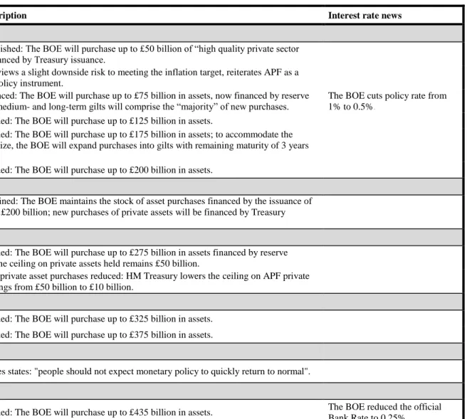
Table VII - Announcements: United Kingdom ... 68
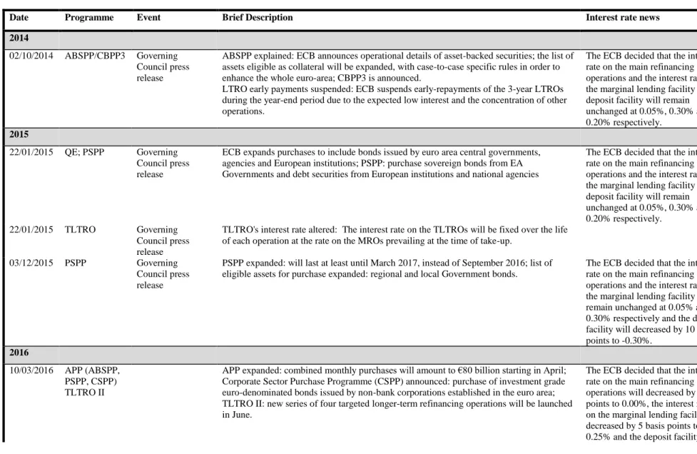
Table VIII - Announcements: Euro Area ... 69
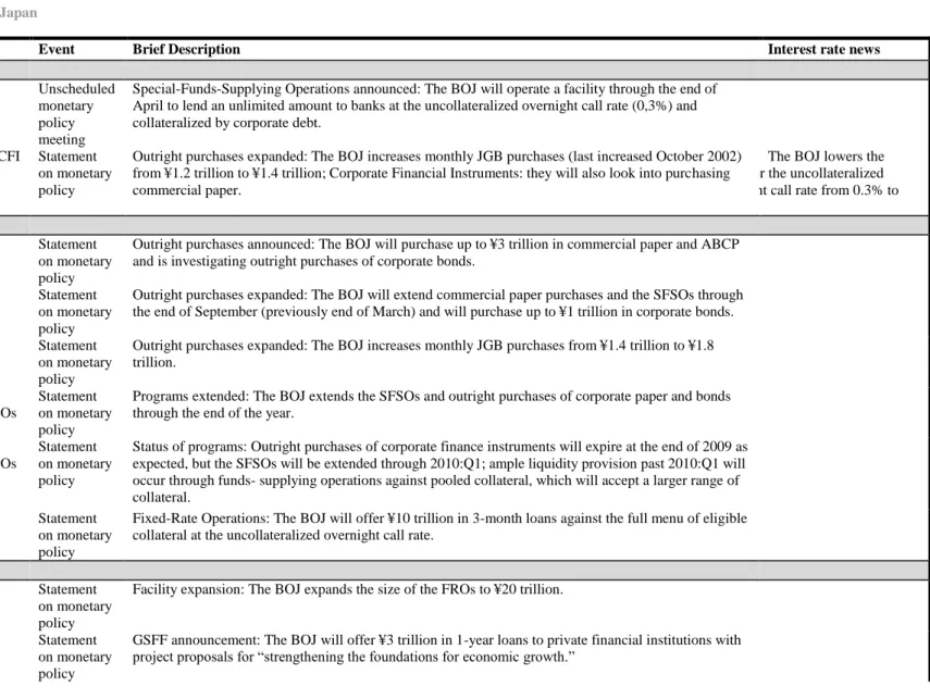
Table IX - Announcements: Japan ... 71
Table X - Results: United States of America ... 74
Table XI - Results: United Kingdom ... 75
Table XII - Results: Euro Area ... 76
1
1. Introduction
On September 2009, the Lehman Brothers announced bankruptcy marking the beginning of what became the “Great Recession”. After this episode, the financial markets became dysfunctional, credit conditions constricted, consumption and investment decreased and overall, the economic indicators deteriorated. Aiming for a recovery of consumption and the economy in general, Central Banks opted to loosen their monetary policy. One of the first actions taken was the decrease of the instrumental rate. The interest rates approached levels close to zero (Zero Lower Bound (ZLB) theory) and financial markets remained dysfunctional. At this point, the conventional monetary policy was worn out so the Central Bank needed a new action plan – the so-called unconventional monetary policies. There are several ways of implementing unconventional monetary policies; this study focuses on the Quantitative Easing measures. Quantitative Easing (QE) is a mechanism where the Central Bank creates new money (electronically) and employs the increasing of monetary base on financial asset purchases, such as government bonds. Before the Financial Crisis of 2007-2009, QE related research was not abundant. After 2008, the amount of studies about the effects of QE skyrocketed. Regarding the US, Gagnon et al. (2011), Chung et al. (2010) and Baumeister and Benati (2010) represent the most cited studies about the effect of QE measures in the American economy. Joyce et al. (2011) and Joyce, Tong and Woods (2011) are relevant essays about the QE programmes lead by the Bank of England (BOE). Some literature on the European case was performed by Attinasi et al. (2009), Gambacorta et al. (2012) and Afonso and Kazemi (2017). The new wave of Japanese QE policies was studied by Rogers et al. (2014) and Gambacorta et al. (2012).
2
Fawley and Neely (2013), Rogers et al. (2014) and Gambacorta et al. (2012) are rare examples of studies that portray and compare the four major QE programmes.
Most of the empirical analysis on the topic uses high-frequency financial data and does not include more than one or two economies. Therefore, there is a lack of literature that describes and compares QE programmes, across Central Banks, especially with theoretical and empirical analysis of its own.
Inspired by the gap on the literature, the aim of this dissertation is to assess the motivations the lead the Federal Reserve System (Fed), the Bank of England (BOE), the European Central Bank (ECB) and the Bank of Japan (BOJ) to consider the use of QE; to portray the peculiarities of each economy and programme and, finally, assess the impact of the announcement and asset purchases under QE policies into the long-term Government bond yield.
The thesis is organized as follows: the following section presents an overview on the relevant literature; section three presents the path through conventional monetary policy to unconventional monetary policy, in particular Quantitative Easing measures; section four describes the model, the data used and the methodology employed for each economy; section five reports the outputs of the empirical analysis and discussion; the conclusion and further research is on section six.
2. Literature Review
The literature on evaluating the impacts of the quantitative easing (QE) programmes has usually obtained its results using high-frequency data. Event-studies and structural vector autoregression (VAR) models are the most used approaches in assessing the impact of unconventional monetary policy. It is worth mentioning the
3
scarcity of studies evaluating the programmes of the United States of America (US), United Kingdom (UK), Euro area (EA) and Japan (JP) with an empirical analysis on their own, and even less studies employing monthly or quarterly data, in order to assess the long-term outcomes of those programmes.
Fawley and Neely (2013) portray the circumstances and motivations that led the Fed (Federal Reserve System of the US), European Central Bank (ECB), Bank of England (BOE) and Bank of Japan (BOJ) to implement QE programmes. A list of the most important announcements made in the scope of QE and a timeline of its purchases is provided. Was concluded that not all QE programmes were implemented with the same goal or tools. The Fed and the BOE chose to expand their monetary bases by purchasing bonds while the ECB and BOJ opted to focus on direct lending to banks. The different type of economy of the countries justifies these differences. The paper presents a valuable conjectural resume of the four major QE programmes using available empirical investigation of the most remarkable literature.
Gambacorta et al. (2012) aimed to measure the effectiveness of unconventional monetary policy at the zero lower bound in eight countries, including Canada, Japan, US and Norway. Using panel VAR with monthly data from 2008 to 2011, it was concluded that the exogenous rise in Central Bank (CB) balance sheets at the zero lower bound leads to a momentary increase in economic activity and consumer prices; in consequence the estimated output effects were qualitatively comparable to the ones found in the literature on the effects of conventional monetary policy, while the impact on the price level is weaker and less persistent; the unconventional measures had a similar macroeconomic effect across countries. Last but not least, the authors assessed
4
that is needed an immense expansion of the CB’s balance sheet to achieve a strong monetary stimulus.
Rogers et al. (2014) used common methodologies in order to report the outcomes of unconventional monetary policy on stock prices, bond yields and exchange rates for the BOE, Fed, ECB and BOJ. The methodology used was an ordinary least squares (OLS) estimator with intraday data and a structural VAR model with daily data. The research concluded that the policies applied were effective, even in the zero lower bound scenarios, improving broad financial conditions. These policies worked mainly through the reduction of the term premia. They observed spill over effects between countries although it was not in the same magnitude for all economies. The authors did not only found good news, the influence of bond yields into assets prices appeared to have a higher effect on the US than in other economies and with the recovery that will be needed after the end of unconventional monetary policies it is likely that the long-term yields will increase.
Joyce, Tong and Woods (2011) evaluate the motivation of the large-scale asset programmes held by the Bank of England and portray how it was executed. The aim is to verify the impact of the asset purchases that began in 2009 had on the economy, specifically in the financial markets. Thus, this paper contributes with a synopsis about the design, operation and impact of the quantitative easing programme of the United Kingdom. The authors emphasise that the scale and speed of the asset purchases indicate that they were made with the intention of reversing the fall in confidence and the risk of rise of inflation falling sharply below target. The architecture of the programme was intended to target purchases of medium to long-term gilts from the non-bank financial sector. The impact was obvious on asset prices. Moreover, it was
5
analysed a variety of approaches used by the BOE’s research to quantify the possible influence of those asset price variances on output and inflation. Although there is no certainty about the exact magnitude of the impact, the evidence suggests that the policy had positive and significant economic effects.
On the same note, Joyce et al. (2011) portray the unconventional monetary measures that the BOE adopted to battle the financial crisis. The study analysed the key transmission channels that affect the financial markets. For this, it was used an event-study analysis and survey data. The authors scrutinize the instantaneous response of asset prices to QE announcements and assign it into separated channels. The assets studied were the gilts, corporate bonds, equities and the Sterling. The majority of the impact of QE on gilt yields happens when the purchases are announced and not when the purchases truly happen. The main results of this study indicate that the QE purchases programs had a noteworthy effect on financial markets and predominantly on gilt yields.
The main goal of Baumeister and Benati (2010) was to analyse the macroeconomics consequences of a reduction in the long-term bond yield spread when the short-term interest rates are constrained by the zero lower bound within the Great Recession (2007-2009) timeframe in US and UK. Their research is guided by two main questions: first, how effective CBs’ unconventional monetary policy actions in the form of government-bonds purchases were in counteracting the recessionary shocks of the 2007-2009 financial crisis; and secondly, how powerful central bank interventions are during the zero lower bound. To answer this question, the article proposes the creation of a counterfactual recreation of how output, inflation and unemployment would have developed if the asset purchases programs did not take place. The research concluded
6
that a reduction in the long-term yield spread employs a prevailing effect on both inflation and output when in a zero lower bound situation, as in the case of the US and the UK.
The focus of Driffill (2016) was the unconventional monetary policy in the Euro zone but it also debates the policies implemented by the Fed and the BOE. The objective was to provide lessons to the Euro area using the information available about the other two programmes. It was noted that, in comparison with the programmes held by the Fed and the BOE, the ECB’s programme had a much smaller effect on bond yields and thus the effects on output and inflation could be less puissant. The good news are that the most common dangers of QE, i.e. the creation of asset prices bubbles, allowing zombie firms and banks to survive, higher levels of future inflation and the deceleration of the adjustment processes, do not appear to be a concern for EA. The ECB’s efforts seemed to contribute on the reduction of costs of debt service that could ease the fiscal situation of member states.
The main contribution for the literature about QE given by Krishnamurthy and Vissing-Jorgensen (2011) was the enlightenment about how different transmissions channels for QE1 in 2008–2009 and QE2 in 2010–2011 led by the Fed influenced the interest rates and their implications in policymaking. The methodology chosen consists in an event-study using intraday data, which allowed the authors to distinguish the various transmissions channels. The methodology used consists in a difference-in-differences approach. The signalling effect, long-term safety channel and the inflation channel were the primary transmissions channels that influenced both QE1 and QE2. The channels that were only relevant during QE1 were the Mortgage-backed Securities (MBS) risk premium, default risk premium and the liquidity channel. Based on these
7
results three main policy implications were derived: it is not appropriate that the spotlight of CBs’ policy rate to be the Treasury rate; QE has a higher benign effect on mortgage and lower-grade corporate rates whenever the Federal Reserve’s asset purchases include non-Treasury assets; and as a Treasury-only policy, such as QE2, is transmitted mainly by a signalling channel, it will make the markets lower the expectation level of future federal funds rates.
Gagnon et al. (2011) clarifies how the Federal Reserve’s large-scale asset purchases (LSAP) were employed and debates the mechanisms through which the asset purchases could affect the economy. The authors quickly examined the experiences of Japan and the UK to compare the results. To assess the effect of LSAP on market interest rates two different approaches were used: an study and a time-series analysis. The event-study analysis consisted in the event-study of eight major announcements using a one-day window frame and it was possible to observe that all interest rates suffered a significant decrease. The event-study and the time-series analysis came to the same conclusions, even using different information in the tests. It was found that the market functioning effect was stronger at the beginning of the LSAP and the portfolio balance effect was probably responsible for the term effects; and that the LSAP resulted in long-lasting reductions in the long-run interest rates on a diverse range of securities even those that were not part of the purchases, indicating a spillover effect.
Wright (2012) opted for a high-frequency event-study and a structural VAR within the period of November 2008 to December 2010, using daily data, in order to measure the impact of the Federal Open Market Committee (FOMC) meetings and announcements related to monetary policy on several long-term interest rates for the US. The conclusions of this work were: monetary policy shocks affect long-run
8
Treasury and Corporate bonds but its effect fades quite fast, in a period of about two months; and the impact of monetary policy shocks were stronger in longer-term interest rates than in short-term interest rates.
Chung et al. (2010) incorporated expectations on the modelling of the impact on macroeconomic variables made by the LSAPs using a forecasting model used by the Federal Reserve Board, from 2009 to 2016. The model made it possible to observe an improvement of real economy conditions that were led by changes in financial conditions, such as lower foreign exchange value of the dollar and higher stock market valuations; LSAPs led to an increase in Gross Domestic Product (GDP), lower unemployment rate and also contributed on price stability, as long-term inflationary consequences of the programme were not a likely scenario anymore. Overall, the study reflects that agents have confidence in the FOMC’s actions.
Attinasi et al. (2009) aim was to discover the determinants of the increase in the sovereign bond yield spread of selected EA countries vis-à-vis Germany. It was done via a dynamic panel regression containing data from several European countries between July 2007 and March 2009. It was observed that announcements of bank rescue packages steered a revision of sovereign credit risk by the investors; and when comparing to Germany, countries with greater expected budget deficits or/and greater government debt ratios had higher government bond yields spreads.
De Grauwe and Ji (2014) scrutinized the changes in Eurozone spreads. The focuses were on outlining how much of the downturn is merited to improving fundamentals and determining how much could be attributed to optimistic market sentiments sparked by the announcement of Outright Monetary Transactions (OMT) in the third quarter of 2012. After analysing nine countries of the EA between the first quarter of 2000 and the
9
third quarter of 2013, the following conclusions derives: throughout 2010-2012 periphery countries suffered an increase in their spread that could not be justified by changes in the fundamentals, such as debt-to-GDP ratio, but by negative market sentiments; after the third quarter of 2012 the spreads of periphery countries have declined and, as before, this occurrence could not be attributed to changes in fundamentals but with the improvement of market sentiments, which coincide exactly with the OMT announcement by the ECB. Thus, market sentiments are not always in line with the fundamentals what could prevent the market from considering the actuals risks.
Studying the relation between banking and sovereign risk in the Euro area was the proposition of Gerlach et al. (2010). In order to do so, the authors questioned what factors have been influencing the spread in the Euro zone after the introduction of the Euro, focusing on the banking sector and sovereign risk. Employing a dynamic panel model with data from nine euro area countries between 1999 and 2009, it was observed that sovereign spreads diminish with bigger equity ratios; the size of the banking sector, proxy by aggregate balance sheet to GDP ratio, was an essential factor of sovereign risk spread relative to Germany in the Euro area; if and when readings of aggregate risk raised, yields increased more rapidly in economies with large banking sectors but the rising in aggregate risk was in itself increasing banking risk. Thus, variations of global risk perception could affect, in size and speed, sovereign risk spreads.
Klepsch and Wollmershäuser (2011) incorporated literature previously mentioned, Attinasi et al. (2009) and Gerlach et al. (2010), on their work about “How the Financial Crisis has Helped Investors to Rediscover Risk” - an analysis of yields spreads on European Monetary Union (EMU) government bonds from 2000 to 2010. The authors
10
used a dynamic panel regression. They observed that spreads converged with the introduction of the Euro and abruptly diverged with the financial crisis of 2007. It is important to note that before the crisis, some spreads’ determinants were being ignored by the investors and after the crisis investors gave more attention to countries’ credit risk. Therefore, risk aversion in the markets became more important. Consequently, during the crisis, the fundamentals turn out to be more important for investors leading to an increase in spreads. As also concluded by Gerlach et al. (2010), sovereign risk is manipulated by equity ratios of banks. At last, the authors additionally concluded that high forecast debt levels have a higher impact on yield spreads than the expected GDP growth rates.
Fawley and Neely (2013), Gambacorta et al. (2012) and Rogers et al. (2014) scrutinize and compare various programmes of unconventional monetary policy. The first study states that purchase of bonds were the main tools used by the Fed and the BOE, while the BOJ and ECB focus on direct lending to banks. Gambacorta et al. (2012) found evidence that the macroeconomic effects were similar among countries and that an immense expansion of the CB’s balance sheet was needed to achieve a strong monetary stimulus. Rogers et al. (2014) observe a higher effect on the US economy than in the others studied and Driffill (2016) argued that the policies of the Fed and the BOE were more effective than the policies of the ECB.
Gagnon et al. (2011) and Wright (2012) agree that QE measures have a greater impact on long-term interest rates comparing with short-term rates.
De Grauwe and Ji (2014) and Klepsch and Wollmershäuser (2011) noticed that fundamentals and spread determinants were being ignored before the financial crises.
11
Krishnamurthy and Vissing-Jorgensen (2011), Gagnon et al. (2011) and Chung et al. (2010) stressed the importance of the confident on the monetary authorities when employing unconventional monetary policies. In the same line of thought, Joyce et al. (2011) concluded that most of the impact on gilts by the QE programmes were at the time of the announcements rather than at the time of the actual purchases.
The entire literature mentioned above is summarized in Table I with results and specific details regarding the methodology and the sample size.
3. The Path from Conventional Monetary Policy to
Unconventional Monetary Policy
Central banks are one of the key agents in every economy. They are responsible for the currency/monetary issuance, supervision of the monetary system and definition and conduction of monetary policy. Different CBs have distinct mandates and so the goal of their monetary policy will be different from one another. In general, the goals of monetary policy (MP) can be price stability, high employment, economic growth, financial market stability, interest rate stability and foreign exchange market stability.
Thus, monetary policy provides ample monetary stimulus to the economy during downturns offers inflationary tension during upturns and eases the sound functioning of money markets.
Although the CB sets the goals for the monetary policy, it is unable to influence it directly. Hence, CBs use their MP tools to manipulate operating targets (such as: banking liquidity, monetary market interest rates) and those targets will influence
12
intermediate targets. These mechanisms will act through transmission channels and will manipulate the final goals of the monetary policy. (Abreu et al., 2012)
The usual action of the CBs is setting target for the overnight interest rate in the interbank money market by adjusting the money supply through open market operations. (Smaghi, 2009) By doing so, the central bank is not involved in direct lending to the Government or the private sector. Therefore, the risk of exposure of the CB’s balance sheet is lessened; the fact that all the transactions that are made to provide liquidity are reverse transactions against a list of eligible collateral also contributes to the low risk incurred in the process. (Smaghi, 2009) As such, CBs conduct the liquidity conditions in the money markets and work on its mandate objectives, piloting key interest rates. (Smaghi, 2009)
Standard and non-standard policies affect the economy through several main transmission channels. The topic will be resumed later through this chapter.
Tension started to build up on American financial markets at the beginning of 2007. In 2008, financial institutions such as Lehman Brothers, one of the biggest investment banks in the world, go bankrupt. As a result, the transmission mechanics of monetary policy stopped working properly as the general risk level went up, resulting in liquidity sinking. Capital flows between countries went to minimum records and the financial crisis rapidly disseminated to Europe and emerging economies.
When the economy suffers a powerful shock the interest rate may be brought to zero or the transmission process of MP may no longer work, even when interest rate different from zero (Smaghi, 2009).1
1 Keynes coined the term Liquidity Trap in 1936 in order to define a situation where the short-term
13
When faced with a scenario where traditional tools are no longer effective, as it happened in the financial crisis of 2007, the policy-makers are challenged with a number of questions. Monetary policy-makers should visibly delineate the objectives of the unconventional measures and then pick the best measures to pursue those objectives. They should also be aware of the possible side effects of those policies, such as the influence on the financial soundness of the CB’s balance sheet and avoiding the blockage of market recovery to normal functioning with unconventional measures. (Smaghi, 2009)
Unconventional monetary policies consist in actions that directly aim the accessibility and cost of external finance to banks, non-financial companies and households. These policies can be funded by CB liquidity, loans, fixed-income securities and equity. (Smaghi, 2009)
The type of shock, the state of the banking system and the differences on institutional peculiarities influence the selection of tools used by the CBs to endure with the atypical scenario in interbank markets and economy in general. (Smaghi, 2009)
In the US, the need for unconventional monetary policy arrived when the economy faced a ZLB situation and the normal status quo was no longer effective. In this case, the unconventional monetary policy substituted the conventional monetary policy.
In the EA, the unconventional monetary policy ensured the transmission of monetary policy in the face of financial market malfunctioning, as a complement of the conventional policies. In the case of ZLB, the CB may decide to influence medium to long-term interest rate expectations, change the composition and/or expand of the CB’s balance sheet. When a transmission tool is not working, the CB may bring the
short-14
term nominal interest rates to zero and step in precisely on the transmission mechanism causing problems using unconventional policies.
Bernanke et al. (2004) found evidence supporting that different financial assets are not perfect substitutes, making variations in the composition of the CB’s balance sheet an effective unconventional monetary policy.
Communication and credibility of the monetary authorities are key aspects to have in consideration when in a ZLB situation. If the CB commits to maintain interest rate at a low level and maintain it at a lower level for longer than previously expected, it should diminish longer-term rates, support other asset prices and stimulate aggregate demand. (Bernanke et al. ( 2004)
There are several ways of applying unconventional monetary policy, such as credit easing, quantitative easing (QE) and manipulations of the exchange rate.
Credit easing aims to reduce specific interest rates and/or rebuild market failures; when the result is the expansion of the money supply it can be taken as a not pure form of QE. (Smaghi, 2009) This instrument can be used when the interest rate is above zero. (Smaghi, 2009) The objective of credit easing is the purchase of certain type of securities as to lower interest rates in specific credit markets, thus the CB hopes to improve the functioning of credit markets and ease the transmissions to the real economy. (Söderström and Westermark, 2009)
Therefore, policies that unusually increase the money base, embracing lending programmes and asset purchases, are called QE measures. Credit easing, which eases credit facilities, can be taken as a special form of QE programme if it increases the monetary base.
15
An alternative way of uplifting the economy is through the depreciation of the exchange rate. The CB could purchase foreign securities and currency, instead of purchasing domestic securities. (Söderström and Westermark, 2009) It is relevant to note that because the exchange rate and inflation expectations are linked, a lower exchange rate will lead to higher inflation expectations and thus lower real interest rates. (Söderström and Westermark, 2009)
Quantitative easing is a measure taken by the CBs with the aim of expanding money supply that affects the liability side of the central bank’s asset side. (Fawley and Neely, 2013) This measure should be only applied when the interest rate is zero or close to it. (Smaghi, 2009)
A quantitative monetary policy aims to influence the money supply. Often described as the central bank balance sheet effects on the asset side. (Söderström and Westermark, 2009)
In order to do so the monetary authority creates money and uses it to purchase financial assets from private investors such as insurance companies, banks and pension funds. Money is created without the need of printing and it is simply achieved by an increase of credit on the central bank’s account. (Delivorias, 2015)
As CBs purchase large amounts of assets, prices rise, thus decreasing by definition the interest rate associated with them. Lower interest rates decrease borrowing costs, increasing investment and consumption. Therefore, it is relevant to understand how the main transmission mechanisms work on affecting asset prices, interest rates and the real economy. (Joyce et al., 2011)
As agents should believe in long-term low policy rates as to lower their expectations of the interest rates, quantitative easing purchases can help those
16
expectations become credible. When the CB buys long-term government bonds it affects the long-term sovereign bond yields and longer-term rates in general, giving a sign that the short-term interest rate will, in fact, be lower in the future. (Söderström and Westermark, 2009)
As seen before, there are several factors influencing how unconventional monetary policy should be executed and how it affects the economy.
As mentioned before, the way through which monetary policy affects the various elements of the economy is called the transmission mechanism and it works across different channels.
The research of how the monetary institutions can manipulate the economy, how the markets react to those actions and what channels allow the standard and non-standard policies to reach the targets settled by the CBs is not a new topic in the economic literature. These topics are again in vogue due to the recent unconventional monetary policies.
The literature is not consensual in which are the most important channels. Below, the channels most seen in the literature will be presented, namely the policy-signalling channel, the portfolio balance channel and the liquidity premia. (Joyce et al., 2011)
The macro/policy news, also known as the signalling channel, denotes to the knowledge that economic agents obtain with announcements of QE and incorporate it into their decisions. This channel can have an ambiguous effect on yields because QE can indicate lower policy rates in the short-run but can signal higher inflation in the long run. (Joyce et al., 2011)
The portfolio balance channel results from the actions that agents do to remodel their portfolio in response to asset purchases made through QE programmes. Another
17
effect of this channel is the increase in the wealth of the agents when the monetary authority buys their assets. (Joyce, Tong and Woods, 2011) Assuming imperfect substitution between assets, a variation of quantity of a specific asset will lead, ceteris paribus, to a variation in its relative expect rate of return. (Joyce et al., 2011) Thus, asset purchases made through QE programmes are expected to decrease bond yields and drive investors to raise their demand on additional long run assets.
Therefore, QE purchases have two main effects through this channel: the increase in assets prices, by diminishing yields that will decrease the cost of borrowing; and an increase in consumption as higher asset prices increase the agents’ wealth. This channel is argued to influence the markets right after the QE announcement and throughout time, as investors need time to rebalance their portfolios. (Joyce et al., 2011)
Assuming that a longer-term asset is riskier than a short-term one, agents ask for a compensation, which is reflected in the price, for holding a long-term asset – the so-called term premium. When the monetary authorities buy this kind of assets, investors will ask for less compensation for holding these assets and term premium will thus fall. A reduction on term premium leads to a reduction of the long-term real rates. (Fawley and Neely, 2013)
The signalling channel affects expected policy rates and the portfolio balance channel reduces the term premium – spreads of long-run interest rates over expected policy rate - and the risk premia – the asked return on riskier assets relative to riskless assets. (Joyce, Tong and Woods, 2011)
A scenario defines a liquid market where there are enough assets for “normal” transactions without shortage, i.e. no difficulty in exchanges. When markets are under stress, they can become illiquid and the liquidity premium – the value asked in order to
18
compensate the agent because of the risk of holding a less liquid asset - may rise. (Joyce et al., 2011) Thus, QE purchases may act through the liquidity premia channel because those purchases may ease and diminish the cost of selling assets that investors face. It is worth mentioning that this channel may only be active during the asset purchases lead by the CB. (Joyce, Tong and Woods, 2011)
As the reader could notice, these mechanisms, although they were analysed separately, produce their outcomes simultaneously. Their strength depends on the economic and financial structure of each economy.
As the aim of this dissertation is to study the effect of unconventional monetary policies into the long-term bond yields, it is relevant to understand the elements of such yield and the mechanisms that may influence it.
Prospects of future policy interest rate variations affect longer-term market interest rates, because these are constructed via the expectations of short-term rates. The impact of market rate variations on rates of long-term maturities (i.e., long-term banking lending rates, 10-year Government bond yields) is less direct than in shorter maturities.
Accordingly, the liquidity premium theory indicates that assets with different maturities are not perfect substitutes. Uncertainty and risk aversion are factors that lead investors to prefer more liquid assets. Risk adverse agents prefer short-run investments as these types of assets have a limited exposure to risk and their capital is stationary for a shorter period. Thus, the long-term interest rate is constructed by the average of the actual and the expected short-run interest rates and the liquidity premium. The liquidity premium is the compensation in return asked by the investors in order to bear the risk of possessing a longer-term and, probably, a less liquid asset. (Abreu et al., 2012)
19
The study of the behaviour of long-term sovereign bond yields has been an important field in the economic world for a long period. Authors have found that its behaviour usually depends on the time span that it is studied, because of economic scenarios.
The credit risk, liquidity risk and the overall risk aversion of agents are factors that Klepsch and Wollmershäuser (2011) refer as relevant for long-term sovereign yields. While Afonso and Rault (2010) studied the role of government balance-to-GDP ratio, the debt-to-GDP ratio, the current account balance ratio, inflation surprises, the real effective exchange rate and a liquidity measure as determinants of long-run sovereign bond yields.
When a country is not in a sound situation and its probability of default is high, investors will demand a higher credit risk premium to reimburse them from holding that risk. Government default risk is considered to result from the fiscal condition of the country because it is usually measured by the debt-to-GDP and deficit-to-GDP ratios. (Klepsch and Wollmershäuser, 2011) In the occurrence of a weakening of the sovereign current account balance, the long-run interest rates might increase. (Afonso and Rault, 2010)
Unconventional measures that are directed at, for example, sovereign bonds will increase the available funds for governments, which will decrease their probability of default. Thus, non-standard policies might decrease long-term bond yields through the reduction of the credit risk.
If an investor suspects that a security will have low demand in poor market conditions, the demanded yield needs to be higher because the agent will require a liquidity premium in order to buy the asset. Thus, mismatches of wills on the financial
20
markets increase transaction costs and will increase the asked yield. (Klepsch and Wollmershäuser, 2011) Generally, a better fiscal position reduces the real long-term interest rate, however, Afonso and Rault (2010) have found that an increase in stocks of government debt diminishes the real interest yield in some countries. Other literature has reached the same conclusions and there might be two reasons for such event: the market may be having a mispricing behaviour, or the market may be welcoming the increase in liquidity. Thus, QE purchases directed at long-term Government bonds may decrease the long-term bond yield. (Afonso and Rault, 2010)
It is worth mentioning that there is not a consensus about the weight of deficit and Government debt on long-term interest rates.
Risk aversion portrays the attitude of investors towards risk. When in times of uncertainty investors tend to be more risk averse. (Klepsch and Wollmershäuser, 2011) Literature usually uses equity market volatility as a proxy for investors’ risk aversion.
Inflation and real exchange rate may be an indicator of monetary authorities’ activity. Sovereign risk may rise in the occurrence of high or expected high inflation. In the study of Afonso and Rault (2010) inflation had a negative relation to real long-term sovereign yields. The real exchange rate also had a negative relation with the long-term bond yield in the majority of the countries analysed.
It is clear that the study of long-term sovereign bond yields has mapped various scenarios, not all consensual.
Unconventional monetary policies are multifactorial, depending not only on the type of shock that happened but also on the approach led by the monetary authorities, the specifications of the economy and the motivations behind the QE programmes. In the next section, each programme will be explained in particular.
21
4. Data and Methodology
The scope of this dissertation is to evaluate the effects of the announcements and the purchases of quantitative easing on the variation of the long-term bond interest rates in the four main economies under quantitative easing measures - United States of America, Japan, United Kingdom and Euro Zone. Expectations are not inside the scope of this dissertation. The period analysed was from 1999 to 2016 for all countries using monthly and quarterly frequency, exceptions may occur.
In this chapter, the general model is presented and design of the QE policies and the methodology will be explained separately by country.
4.1. The Model
To obtain the answers proposed by this study it was decided to employ a regression using the target variable, the factors that influence it and QE specific variables. After analysing the literature on the determinants of the yields and the yields spreads, it was possible to compile the most important elements used for the analysis.
Several authors have shown that the main determinants of the long-term Government bond interest yields are the credit risk and the investors’ risk aversion. Besides those determinants, other factors must be taken in consideration when measuring the effect of unconventional monetary policies into the variation of the yields, such as international risk, the economic cycle, the stance of monetary policy, real effective exchange rate and last but not least, the announcements and actions of outstanding monetary measures. In order to measure these determinants and actions one must use proxies. Below follows
22
the explanation for the specific variables used, concluding with a general model that serves as a base for the country-by-country analysis showed afterwards in this chapter.
The chosen dependent variable is the variation of the long-run Government bond yield with 10 years of maturity. The dependent variable and the lagged level of the long-term Government bond yield are included in the left-hand side of the regression. As a representation on the stance for conventional monetary policy, the instrumental rate for each economy is used.
The credit risk, as explained on the ECB monthly report of May 2014 (ECB, 2014), is classically related with country ratings and default risk of a specific country. Debt and deficit-to-GDP ratio, structure of debt maturity, interest expenditure-to-GDP or interest expenditure-to-tax revenue ratios usually measure it. In the model it will be used the Debt-to-GDP ratio in order to measure sovereign’s credit risk. During the tests, manipulations of this indicator were used, such as the growth rate and the variation comparing with the previous period analysed.
The aggregate banking assets-to-GDP ratio and the banking equity-to-assets ratio which together represent the total assets held by the financial sector are the variables used by (Gerlach et al. (2010) and Klepsch and Wollmershäuser (2011) in order to assess the impact of the sovereign risk channel into the long-term interest rate. When possible these variables will be used in addiction of the typical debt-to-GDP ratio.
Several proxies are used to evaluate the investors’ risk aversion. Klepsch and Wollmershäuser (2011) explain that corporate bonds spreads and equity market volatility are used to size investors’ risk aversion. In the same line of thought, the ECB (2014) specifies that US corporate bond spreads and US stock market implied volatility
23
(VIX) are both valid proxies. Gambacorta et al. (2012) explain that the VIX is an indicator of financial turmoil and economic risk and adds that it should capture uncertainty shocks that may have affected the “macro financial dynamics” throughout the crisis. Thus, the variable chosen was the VIX index, which weights the volatility of the US equity market.
As a control variable to regulate for economic cycles, the industrial production index (INDPRO) is used because it proxies output. (Peersman, 2011) During the tests, manipulations of this indicator were used, such as the growth rate and the variation comparing with the previous period analysed.
Afonso and Kazemi (2017) found evidence that the effective exchange rate is a determinant of the long-term sovereign yield in the Euro area. Thus, it is be included in the study as to observe if it is also a determinant on the other economies studied.
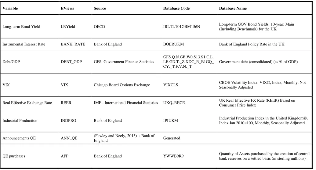
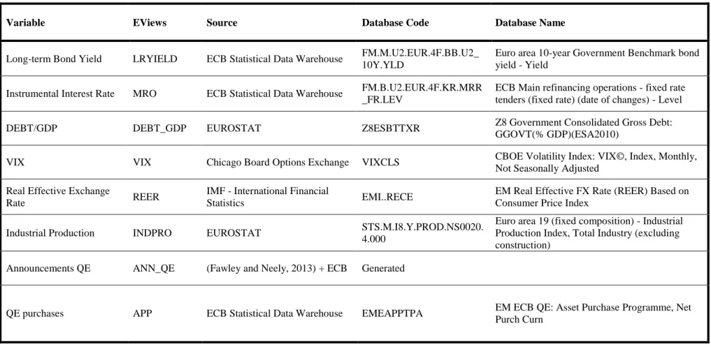
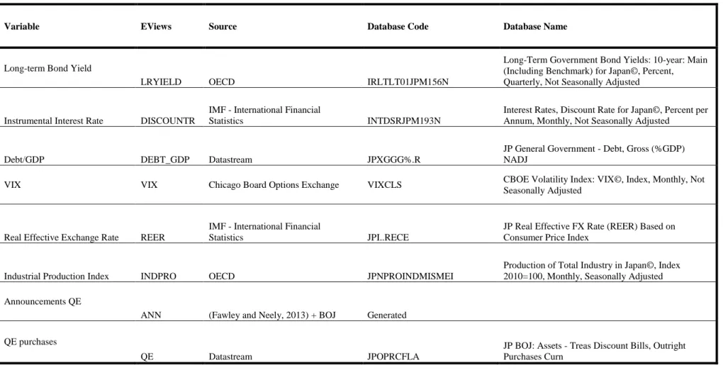
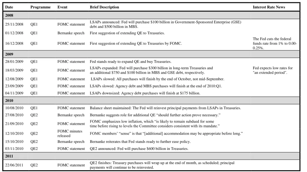
Last but not least, the announcements related with QE and the respective purchases are the variables used to measure the unconventional monetary policy in study, i.e. Quantitative Easing. Therefore, a dummy is created, called ANN that will take the value 1 when CBs make announcements of QE programmes in that month and 0 otherwise. The variable QE will take the value of the asset purchases made by CBs in the months that the actual purchases occurred in the respective currency of the economy being treated at the time. Tables VI, VII, VIII and IX scrutinize the announcements considered for the empirical analysis.
For a full list of the variables used, their time series name, database and nomenclature on EViews, consult tables II, III, IV and V in the appendix.
24
Placing together the variables mentioned above in a regression equation and taking into consideration the high persistence of financial time-series, the following regression is used to assess the effect of Quantitative Easing into the variation of long-run Government bond interest yields:
∆ ( 𝐿𝑅 𝐺𝑜𝑣 𝑏𝑜𝑛𝑑 𝑌𝑖𝑒𝑙𝑑) t = 𝛼 + 𝛽1 (𝐿𝑅 𝐺𝑜𝑣 𝑏𝑜𝑛𝑑 𝑌𝑖𝑒𝑙𝑑) t + 𝛽2 𝑃𝑜𝑙𝑖𝑐𝑦 𝑅𝑎𝑡𝑒 t + 𝛽3𝐷𝐸𝐵𝑇𝐺𝐷𝑃 t + 𝛽4 𝐴𝑔𝑔𝑟𝑒𝑔𝑎𝑡𝑒 𝐵𝑎𝑘𝑖𝑛𝑔 𝐴𝑠𝑠𝑒𝑡𝑠 𝐺𝐷𝑃 t + 𝛽5 𝐵𝑎𝑛𝑘𝑖𝑛𝑔 𝐸𝑞𝑢𝑖𝑡𝑦 𝑇𝑜𝑡𝑎𝑙 𝐵𝑎𝑛𝑘𝑖𝑛𝑔 𝐴𝑠𝑠𝑒𝑡𝑠t + 𝛽6 𝑉𝐼𝑋 t + 𝛽7 𝐼𝑁𝐷𝑃𝑅𝑂 t + 𝛽8 𝑅𝐸𝐸𝑅 t + 𝛽8 𝐴𝑁𝑁 t + 𝛽9 𝑄𝐸 t + 𝜀𝑡 ,
with t = 1, …, 204 denoting the monthly time dimension or t = 1, …, 68 denoting the quarterly time dimension depending on the time period being analysed. Including 𝛼 that denotes the constant and 𝜀 denoting the error term for all models.
The econometric tests were conducted using the statistics software EViews 9. For all the estimations, an OLS regression was employed with HAC correction for standard errors and covariance.
4.2. Methodology
The model was built crossing references about the determinants of the long-term Government bond yield and QE policies and so there is not a framework to strictly follow. The goal is to find the most significant explanatory variables for the variation of the long-term Government bond yield on the time spans used, which can lead to different variables employed for different countries. Thus not resulting in a uniform model but in the most explanatory model possible given the economy and period analysed. In order to do so, sub-time samples are employed and all the explanatory
25
variables are tested (including lags, growth rates, variations) and then selected in order to find the determinants that compose the best the variation of the long-run Government bond yield.
Four models specifications compose the analysis:
Entire time sample: 1999/2000 to 2015/2016;
Time sample: 1999/2000 to 2007;
Time sample: 2007 to 2015/2016;
Time sample: 2007 to 2015/2016 – only QE related variables.
On the appendix is presented the mandate of the CB in question, some of the roots for the crisis, a timeline of the QE measures and the four regressions resulting from the empirical analysis, for the four economies feathered in this essay.
5. Results and Discussion
In this section, the results for each group will be presented and discussed. From here the coefficients are present with three decimal places. The exact numbers are in the related tables of each economy in the attachment sections of this dissertation.
5.1. United States
In the current section it is presented the results of the empirical analysis and discussion for the US economy. In order facilitate the interpretation, the following categorization will be used to address the regressions used:
26
1M: 1999 M04 – 2007 M12 1Q: 1999 Q3 – 2007 Q4
2M: 2008 M01 – 2015 M12 2Q: 2008 Q1 – 2015 Q4
3M (QE only): 2008 M01 – 2015 M12 3Q (QE only): 2008 Q1 – 2015 Q4
4M: 1999 M03 – 2015 M12 4Q: 1999 Q3 – 2015 Q4
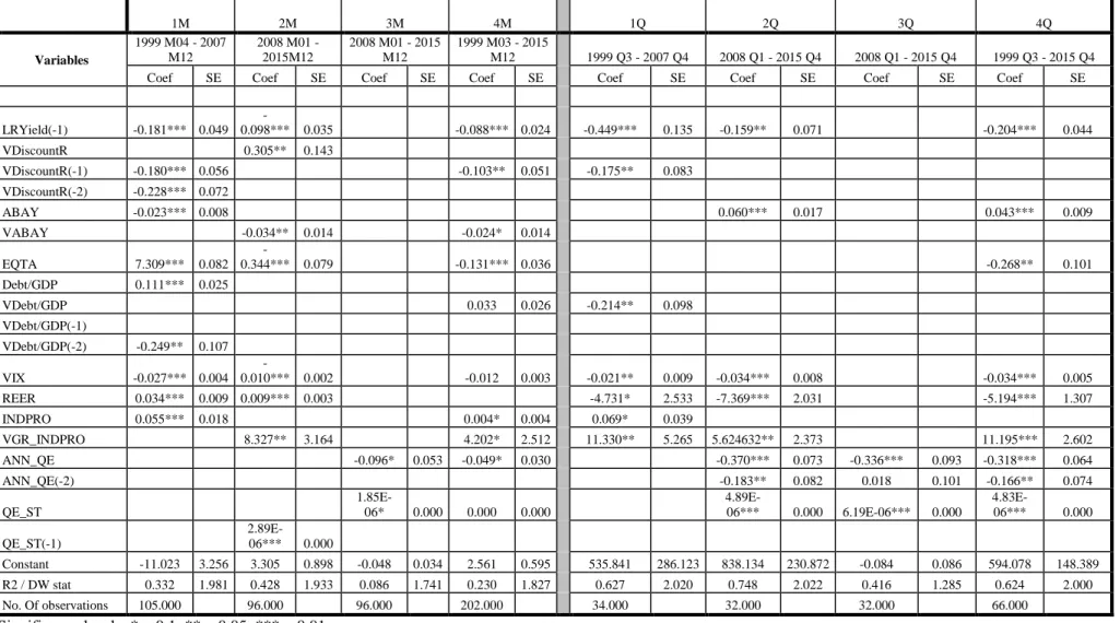
Across all regressions of both time frequencies the LRYield(-1) presents a negative coefficient, which can be explain by the construction of the VLRYield itself: VLRYield = LRYield – LRYield(1). The value of the coefficient ranges between 0.449 and -0.088.
The variation of the instrumental rate (VDiscountR = DiscountR – DiscountR(-1)) has a negative coefficient for the regression 1M (VDiscountR(-1) = -0.189; VDiscountR(-2) = -0.228) and 4M (VDiscountR(-1) = -0.103) and a positive coefficient for the regression 3M (VDiscountR(-1) = 0.305). A different variable used in the literature as a proxy for the stance of MP is the effective federal funds rate. However, as it was not statically significant (SS) in the regressions tested and it was removed from the analysis. This happened because, although the Fed sets a target on the EFFR, the DiscountR is the tool used by the Fed to manipulate the money supply and achieve the EFFR target.
As explained before, ABAY, EQTA, and Debt/GDP are measures for sovereign’s credit risk. The size of the banking sector within a country, ABAY, has a statistically significant and positive coefficient on equation 2Q (0.060) and 4Q (0.043) and a statistically significant and negative coefficient on equation 1M (-0.023). VABAY presents a negative coefficient on equation 2M (-0.034) and 4M (-0.024), while in the other equations, it was not statistically significant and thus it was removed from those
27
regressions. EQTA presented a positive coefficient on 1M (7.309) and a negative coefficient on 2M (-0.345), 4M (-0.131) and 4Q (-0.267); in the other equations, it was not statistically significant. One possible explanation for the positive coefficients for the size of the banking sector within a country and the banking equity-to-banking assets ratio is that the recovery of the banking system improved the yields and consequently the VLRYield. (Klepsch and Wollmershäuser, 2011) On the other hand, a negative coefficient may represent that a higher-sized banking system or a decrease of equity regarding the banking assets indicates a more fragile banking sector with a higher risk of bank default and as bank rescue packages have a negative impact in the economy, the VLRYield increases.
The Debt/GDP represents the Government’s default risk. A higher value indicates a higher probability of default, which, in theory, leads to an increase of the VLRYield. (Klepsch and Wollmershäuser, 2011) Debt/GDP has only retrieved a SS positive coefficient on equation 1M (0.111), while VDebt/GDP has a negative coefficient on 1Q (-0.214).
The indicator for financial turmoil presents negative coefficients in all equations (between -0.011 and -0.034), although not being statistically significant on 4M. A negative relation between VIX and VLRYield may indicate that investors prefer long-run instruments when financial markets are not sound.
The real exchange rate was statistically significant through monthly and quarterly analysis, with the exception of equation 4M. On the monthly analysis, the coefficient was positive (in 1M: 0.034 and in 2M: 0.009), while in the quarterly analysis it presents a negative coefficient (in 1Q: -4.731, 2Q: -7.369 and in 4Q: -5.194). The signal of the coefficient for REER is not consensual through the literature. For example, Afonso and
28
Rault (2010) obtained positive and negative relations between these variables, mostly negative for the countries analysed. In this study, the REER was significant in more expressions using quarterly data than with monthly data and the coefficients were higher.
The variables used to measure output (INDPRO and VGR_INDPRO) were always SS, displaying a positive relation with the dependent variable. The positive relation reflects the increase on LRYields due to the improvement of the overall economy measured by the industrial production index. The VGR_INDPRO (between 11.330 and 4.201) has a much higher coefficient than INDPRO (between 0.069 and 0.004), which may be explained by the lag between the announcement of the indicator and the necessity of adapting expectations by the agents on the VLRYield.
Across the monthly and the quarterly analysis, two variables were used to assess the impact of the announcement of QE: ANN_QE and ANN_QE(-2). ANN_QE gave a SS negative relation in equation 3M (-0.100), 4M (-0.050), 2Q (-0.370), 3Q (-0.336) and 4Q (-0.318), while ANN_QE(-2) was only significant and negative on the quarterly equations 2Q (-0.183) and 4Q (-0.318). Although it did not retrieve the expected signal on 3Q, it was not statistically significant. Overall, the announcement of QE policies decreased the VLRYield, as seek by the authorities.
The variables used to represent the purchases made under the QE policies were: QE_ST, QE_ST(-1), QE_CT and QE_CT(-1). As both variations gave the same coefficients, QE_ST and QE_ST(-1) were chosen as they produced better outputs in term of overcoming auto-correlation problems. QE_ST had a positive coefficient on 3M (1.85E-06), 4M (1.27E-06 but not SS), 2Q (4.89E-06), 3Q (6.19E-06) and 4Q (4.83E-06).
29
In the US’s case, the estimations made under the quarterly frequency performed better than the ones made on the monthly basis as they presented a higher R2 and Durbin-Watson statistics closer to two.
Reviewing the results, the effect of QE policies on the VLRYield was not clear in sign and presented modest coefficients.
The results for the United States are presented in table X.
5.2. United Kingdom
The results of the empirical analysis and discussion for the UK are presented in this section. For ease of reading, the following nomenclature will be used to address the regressions executed:
1M: 2000 M03 – 2007 M12 1Q: 2000 Q2 – 2007 Q4
2M: 2008 M01 – 2016 M05 2Q: 2008 Q1 – 2016 Q1
3M (QE only): 2008 M01 – 2015 M12 3Q (QE only): 2008 Q1 – 2017 Q1
4M: 1999 M06 – 2015 M01 4Q: 2000 Q2 – 2016 Q2
The LRYield(-1) presents a negative and statistically significant coefficient on 4M (-0.085) and 2Q (-0.246); and LRYield(-2) in 1Q (-0.244) and 4Q (-0.233). This can be explain by the construction of the VLRYield itself: VLRYield = LRYield – LRYield(-1). The VLRYield(-1) has a positive relation with the dependent variable and it was only statistically significant on 1M (0.219) and 2M (0.284). The VLRYield(-2) presents a negative coefficient of -0.176 significant at the 10% level. The variation of the LRYield was not statistically significant on the quarterly basis analysis and thus it was removed from the estimations.
30
The variation of the instrumental rate in UK’s case is the bank rate (VBankRate = BankRate – BankRate(-1)). The first lag of this variation is SS and has a negative coefficient for the regression 1M (-0.317), 1Q (-0.487) and 4Q (-0.173); while the second lag has a negative relation with the dependent variable on equation 2M (-0.234) and 2Q (-0.232). Therefore, this variable does not present the expected relation with the VLRYield, as the CB decreases the BankRate (= VBankRate) in order to decrease the long-term interest rates and consequently the LRYield and the VLRYield.
The indicators for sovereign risk used were VDebt/GDP, VDebt/GDP(-1) and VDebt/GDP(-2). VDebt/GDP was the only statistically significant variable, presenting a positive relation with the dependent variable on equation 1Q of 0.127: an increase/decrease on VDebt/GDP leads to an increase/decrease on VLRYield.
The VIX retrieved a negative coefficient in all the equations, although not SS on 1Q. The coefficient was rather small: varying from -0.006 to -0.032. As seen before on the US case, a negative relation may hint that investors swift their demand from short-term riskier assets to safer assets such as the Government bonds, thus increasing the liquidity of Government bond assets and lowering its yield.
The real effective exchange rate (REER) was not statistically significant in any regression across both time frequencies.
The proxy for output INDPRO presents a positive (and SS) relation with the VLRYield on equations 4M (0.011) and 1Q (0.081). The VGR_INDPRO has a SS negative coefficient of -0.808 when analysed for the period 2000-2007 on a quarterly basis. Some literature about the determinants of the long-term Government bond yields, such as Gerlach et al. (2010), found evidence that in the period previous to the financial
31
crisis (2000 – 2007), the fundamentals were being underrated by the investors, which can explain the negative relation between the VGR_INDPRO and the VLRYield on 1Q.
In order to appraise the impact of the QE policies on the VLRYield, the following variables were used: ANN_QE (t=0,-1,-2,-3) and AFP (t=0,-1,-2,-3). Regarding the announcements of QE: ANN_QE presented a negative coefficient, which was not statistically significant. Only ANN_QE(-1) presented a SS positive coefficient of 0.22 on 2Q and 0.31 on 3Q. The variables used to measure the effective purchases of assets under QE measures did not present homogenous signals for the coefficients. The AFP showed a positive SS coefficient, although small, of -1.91E-06 on equation 1Q. The AFP(-1) has a small but positive SS coefficient on 3M (1.58E-07) and 2Q (1.32E-06). The AFP(-2) presents a SS negative coefficient of -6.61E-08 on 2M and of -1.04E-07 on 4M. Last but not least, the AFP(-3) has a SS positive and small coefficient on 3M of -1.75E
-07.
The effect of QE policies on the VLRYield is not clear due to its small coefficients and opposite signs throughout the estimations.
In the UK’s case, the estimations made under the quarterly frequency performed better than the ones made on the monthly basis as they presented a higher R2 and Durbin-Watson statistics closer to two. However, it was not possible to obtain more statically significant variables than in the monthly analysis.
The results for the United Kingdom are presented in table XI.
5.3. Euro Area
In this section, the outputs from the regressions about the EA are presented.
To facilitate the reading, the following cipher will be used to address the regressions executed:
32
1M: 2000 M02 – 2007 M12 1Q: 2000 Q1 – 2007 Q4
2M: 2008 M01 – 2016 M12 2Q: 2008 Q1 – 2016 Q4
3M (QE only): 2008 M01 – 2017 M02 3Q (QE only): 2008 Q1 – 2017 Q1
4M: 1999 M04 – 2017 M01 4Q: 2000 Q3 – 2016 Q4
The first variables analysed were the LRYield in its lagged (t = -3) form, and the VLRYield (t = -2 and t = -3). The LRYield(-3) has a negative but not statistically significant coefficient on 1M, while the VLRYield(-1) displays a negative relation on 1Q and a positive on 1M and 2M, though never presenting SS coefficients for these equations. This variable presented SS positive coefficients on 4M (0.140), 2Q (0.213) and 4Q (0.25). The VLRYield(-2) has a negative, but not SS, coefficient on 1Q and a negative relation (-0.164) significant at the 10% level.
The instrumental rate – the main refinancing operations rate (mro) – retrieved outputs with opposite signs, but when comparing their magnitudes it resulted in an overall positive relation: a decrease/increase on the policy rate leads to a decrease/increase on the VLRYield. The mro(-3) has a positive (0.245) SS relation with the dependent variable. The VMRO delivered a positive non-SS coefficient on 4M and a SS negative coefficient (-0.208) on 1M; while VMRO(-1) displayed a negative but not SS coefficient on 2M and a SS positive coefficient (0.357) on 2Q.
Conventional theory indicates that higher levels of Debt/GDP increase a country’s default probability leading to investors requiring a term premium in order to buy Government bonds, which further leads to higher rates for these instruments. Recent literature about the influence of the fundamentals on the process of expectations of the financial agent has sparked after the financial crisis in 2007-2009. Gerlach et al. (2010) and Klepsch and Wollmershäuser (2011) found evidence that agents may have under
33
looked the impact of Debt/GDP on periods previous to the crisis. The results found in this essay support that theory for the EA. The Debt/GDP(-1) presented a negative SS coefficient (-0.077) on 1Q (2000 Q2 – 2007 Q4) with the VLRYield, while VDebt/GDP presented a positive SS relation (0.084) on 4Q (2000 Q3 – 2016 Q4); and GR_Debt/GDP presented a positive SS coefficient of 12.299 when analysed for the 2008 Q1 – 2016 Q4 timeframe.
The VIX presented a negative relation in all equations which was only SS on 2M, 1Q, 2Q and 4Q with coefficients ranging from -0.003 to -0.028.
The analysis of the impact of the real effective exchange rate (REER) on the VLRYield revealed a negative influence on the period before the crisis (1M and 1Q) and a positive relation when analysed from 2008 to 2016 (2M and 2Q). Supporting that REER is a determinant of the sovereign yields in the EA, as found by Afonso and Kazemi (2017).
Overall, the INDPRO variables displayed a positive relation on the periods before the crisis (1M and 1Q): an increase/decrease of the industrial production index leads to an increase/decrease on the variation of the long-term Government bond yields (VLRYield). In particular, the GR_INDPRO has a strong coefficient of 14.399 significant at a 5% level.
Finally, the QE measures are represented by: ANN_QE(t = 0, -1, -2 and -3) and APP(t = 0, -1, -2 and -4). On a monthly basis, ANN_QE(-1) displays a negative SS relation with the dependent variable (-0.096);ANN_QE(-2) also has a negative coefficient of -0.151 on 2M and -0.141 on 4M. On a quarterly basis, only the ANN_QE(-2) is SS with a positive coefficient of 0.299 on 4Q.
34
The asset purchases under QE programmes generated coefficients with opposite signs across the empirical analysis. The APP(-1) has a small positive SS coefficient on 2M. The APP(-2) also has small positive coefficients, which are SS on 3M and 4M. The APP(-4) was the only variable of this group to provide a negative SS coefficient on the estimations – it has a negative coefficient of -4.16E-06 on 3M and of -6.34E-06 on 4M. On a quarterly basis, the APP(-4) is the only variable with a statistically significant coefficient. It displayed a negative coefficient of -1.47E-06 on 4Q.
The equation exclusively with QE related variables on a monthly basis – 3M – have only two statistically significant variables with opposite directions and similar magnitudes: APP(-2) and APP(-4). No QE related variables were statistically significant on the homologous equation on a quarterly basis (3Q).
In the Eurozone’s case the quarterly regressions provided better R2 and
Durbin-Watson statistics than the regressions tested on a monthly basis. The results for the Euro Area are presented in table XII.
5.4. Japan
In this section, it is presented the results and discussion from the empirical study regarding the Japanese case.
For ease of reading, the following nomenclature will be used to address the regressions executed: 1M: 1999 M05 – 2007 M12 1Q: 2000 Q2 – 2007 Q4 2M: 2008 M01 – 2015 M12 2Q: 2008 Q1 – 2015 Q4 3M (QE only): 2008 M01 – 2015 M02 3Q (QE only): 2008 Q1 – 2015 Q4
35
4M: 1999 M06 – 2015 M01 4Q: 1999 Q4 – 2015 Q4
The variables regarding the LRYield were only statistically significant on equation 2Q. The LRYield(-2) presents a negative coefficient of -0.956 significant at 1% level. While LRYield(-3) has a positive coefficient around 0.178 at a 10% significance level. Overall, the effect of the lags LRYield on the dependent variable is negative, as expected due to the construction of the VLRYield itself: VLRYield = LRYield – LRYield(-1).
The VLRYield(-2) displays a negative relation (-0.185) on 4M at 1% significance level (-0.167) on 4Q at 5% significance level. The VLRYield(-4) has a negative coefficient on 4M (-0.145) significant at the 5% level. The lags of the dependent variable were not SS in any other regression.
The instrumental rate used by the BOJ is the DiscountR. A decrease/increase of the DiscountR should decrease/increase the LRYield. Thus, a decrease/increase of the VDiscountR should decrease/increase the VLRYield. The VDiscountR(-2) has a negative coefficient of -0.367 on 4Q and is SS at the 5% level, while on 2M it presents a positive relation (0.812) with a significance level of 1%. The VDiscountR(-1) has a SS positive coefficient on 2Q and the VDiscountR(-3) has a SS positive on 1M. By analysing the magnitudes and the signs of the variables, it can be concluded that the VDiscountR evolves in the same direction as VLRYield, indicating that the monetary policies may have an impact on the long-term Government bond yield.
A lower Debt/GDP ratio indicates sound public finances and a lower LRYield. In theory, the variables Debt/GDP, VDebt/GDP and GR_Debt/GDP should evolve in the same direction as the variable in study. Statistically significant and negative relations