Abstract— This work focus on a coexistence study between
wireless microphone systems and secondary users of the TV White Spaces, using a Monte-Carlo methodology. Exclusion areas around wireless microphone receivers, for co-channel and adjacent channel interference, are computed, considering indoor and outdoor scenarios. Using this methodology, impact and tendencies of several parameters over the probability of interference are analyzed, like spectral channel spacing, separation distance and propagation scenario. As an example, for outdoor scenarios, the spectral spacing between primary system and secondary users, ranging from 0 MHz (co-channel operation) to 16 MHz (2 DVB-T channels) results in a protection distance of 13.9 km and 2.2 km, respectively.
Index Terms—Cognitive radio, Frequency modulation,
Microphones, Radiofrequency interference, UHF propagation.
I. INTRODUCTION
V White Space (TVWS) cognitive device operation within the UHF bands may be permitted if (and only if) it does not interfere with incumbent services operation, such as DVB-T broadcast and wireless microphone systems [1]. TVWS devices should either sense the presence of other signals or make use of a geolocation database to determine which spectrum is unused in the vicinity [2]. Recent studies have shown however that the signal levels they would need to sense down to are extremely low, making the task difficult to accomplish with existent mobile technology [3]. Geolocation database is nowadays the most promising alternative to sensing. With this approach, TVWS device provides their location, and receives information on frequency and power levels they can use.
One of the issues in developing a geolocation approach is to define a methodology that enables the database to derive such Manuscript received September 13, 2011. The research leading to these results has received funding from the European Community’s Seventh Framework Programme (FP7/2007-2013) under grant agreement No. 248560 (COGEU). R. P. Dionísio gratefully acknowledge the Portuguese Foundation for Science and Technology (FCT) through grant SFRH/PROTEC/50015/2009 for funding his PhD.
R. Dionisio is with Instituto Politécnico de Castelo Branco, Av. do Empresário, 6000-767 Castelo Branco Portugal (phone: +351-272-339-399; fax: +351-272-339-399; e-mail: [email protected]).
P. Marques and J. Rodriguez are with Instituto de Telecomunicações, Campus de Santiago, 3810-193 Aveiro Portugal (e-mail: [email protected], [email protected]).
a list that could be available for TVWS devices. To protect incumbent services against interferences, depending on the transmit power of the TVWS device, a minimum distance to the closest possible receiver working at the considered channel, is required.
Studies based on interference simulations and device parameters were conducted in [4], to compute protection distance for DVB-T receivers. They present a methodology to populate a geolocation database with available frequency and maximum power that a TVWS device could use, without causing interference. This paper will focus on the protection of wireless microphones systems.
From the wireless microphone industry, one of the most demanding systems in terms of quality of service and bandwidth are Professional Wireless Microphone Systems (PWMS). PWMS need to provide a high audio quality with 100 % duty cycle. They are used indoors and outdoor, with fixed or mobile equipment. The expected audio quality needs to be completely reliable, i.e. PWMS need to stay above the quality threshold all the time [3]. Such stringent specifications are very different to communication systems, where a certain amount of errors (BER) may be allowed. Moreover, PWMS equipment may be operated everywhere and at any time, especially in case of “breaking news” events leading to different situations to be considered.
The objective of this paper is to measure the influence of TVWS’s secondary users to wireless microphone systems, and compute exclusion areas around wireless microphone
Interference Study Between Wireless
Microphone Systems and TV White Space
Devices
Rogerio Dionisio, Member, IEEE, Paulo Marques, and Jonathan Rodriguez
T
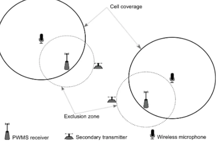
receivers, as depicted in Fig. 1. Section II describes the methodology used to compute the probability of interference. Section III and IV present parameter values and examined scenarios. Section V follows with simulation results, where we discuss the impact of wireless microphones activity on the availability of TVWS. Conclusions are finally drawn in Section VI.
II. METHODOLOGY
The criterion used for interference to occur is to have a carrier to interference plus noise ratio (C/(N+I)) less than the minimum allowable value. In order to compute the C/(N+I) of the PWMS receiver, we need first to establish the signal from the wireless microphone, corresponding to the C, the signal produced by the interfering transmitter, corresponding to the I, and the thermal noise, corresponding to the N. This is done defining technical parameters for each system; this includes the receiver and transmitter specifications, the propagation model associated with the medium of communication and a measure of the quality of service required. The position of the wireless microphone and the PWMS receiver is identified and a link budget is computed. The same process occurs for the interfering system. Having knowledge of both the primary signal and the interfering signal allows the PWMS receiver C/(N+I) to be computed, using a Monte-Carlo technique.
SEAMCAT - Spectrum Engineering Advanced Monte-Carlo Analysis Tool [5], from CEPT, is used to study the interference between PWMS systems and White Space Devices (TVWS) secondary users. For each trial, the received primary signal C is compared to the sensitivity S of the PWMS receiver. If C falls below S, the trial is discarded. Then, if C/(N+I)trial is higher than C/(N+I)target, no interference is
registered; Otherwise, interference occurs and this event accumulates to the number of trials with the same result (NInt). Finally, after all trials are computed (NAll), the probability of interference is expressed as
𝑃!"#$%&$%$"'$= 𝑁!"# 𝑁!"". (1)
Fig. 2. Maximum interference levels as a function of the frequency offset, for a 200 kHz channel PWMS receiver.
TABLEI
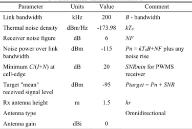
PWMSRECEIVER SPECIFICATIONS
Parameter Units Value Comment Link bandwidth kHz 200 B - bandwidth
Thermal noise density dBm/Hz -173.98 kT0
Receiver noise figure dB 6 NF
Noise power over link bandwidth dBm -115 Pn = kT0B+NF plus any noise rise Minimum C/(I+N) at cell-edge dB 20 SNRmin for PWMS receiver Target "mean"
received signal level
dBm -95 Ptarget = Pn + SNR
Rx antenna height m 1.5 hr
Antenna type Omnidirectional
Antenna gain dBi 0
This way, we are able to quantify the probability of interference between PWMS and TVWS, considering many independent simulation trials.
III. PRIMARY AND SECONDARY USERS SPECIFICATIONS A. Incumbent user
The PWMS link is defined in such a way that the receiver is at the edge of the coverage area with the received signal equal to -95 dBm [3]. The criterion for interference to occur is for the PWMS receiver to have a carrier to interference plus noise ratio, C/(N+I), less than the minimum allowable of 20 dB [3]. A summary of the specifications for the WM receiver is shown in Table I.
At the WM receiver, maximum co-channel interference permitted should be below -115 dBm, taking as a basis analogue FM wireless microphone systems [3]. Fig. 2 represents the absolute power level (in dBm) of maximum interfering signal, which might be tolerated by the receiver at a given frequency separation.
Fig. 3. TVWS UE equipment emission masks normalized to 1 MHz measurement bandwidth. 0 0.2 0.4 0.6 0.8 1 −120 −110 −100 −90 −80 −70 −60 −50 −40 −30 −20 Frequency Offset (MHz) Maximum Interference (dBm) 0 2 4 6 8 10 12 −30 −25 −20 −15 −10 −5 0 Frequency Offset (MHz) Emission Mask (dBc) WSD UE
TABLEII
TVWSUE TRANSMITTER TECHNICAL PARAMETERS
Parameter Units Value Comment
Link bandwidth MHz 5 LTE 5 MHz
In-block EIRP dBm 23 P
Tx antenna height m 1.5 ht
Antenna type Omnidirectional
Antenna gain dBi 0
B. Secondary user
While TVWS devices technology is still unknown, 3GPP Long Term Evolution (LTE) standard [6] operating over TVWS is used as proxy for the secondary user of the spectrum. This study considers only user equipment (UE) transmitters as a source of interference, due to their mobility and conceivable proximity with PWMS systems. Antenna pattern is assumed to be omnidirectional in azimuth and elevation. Spectral emission mask are illustrated in Fig. 3, which is also based on the 3GPP standard [6] that defines the maximum Out-of- Band (OoB) emission limits for UE.
We also consider that TVWS transmitters are continuously emitting at a maximum power of 23 dBm (5 MHz bandwidth) to account for interference in a worst-case scenario. Table II shows a summary of the technical parameters used.
IV. SIMULATION SCENARIOS
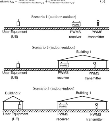
Several scenarios with different characteristics are needed to get acceptable results from interference simulations. Therefore, we consider three deployment geometries, as depicted in Fig. 4:
• Scenario 1: Primary and secondary user outdoors; • Scenario 2: Primary user outdoor and secondary user
inside a building;
• Scenario 3: Primary user and secondary user inside different buildings.
All simulation scenarios are composed with one primary system (PWMS) and one secondary system (TVWS UE), each of them is composed of one transmitter and one receiver. We also consider that the central frequency of all systems corresponds to the centre of a DVB-T channel. For adjacent-channel interference scenarios, spectral separation is measured between the central frequencies of both systems.
A. Propagation Model
Wireless microphone signals almost never operate under free space conditions. Therefore, in addition to the free space path loss, signals are subject to additional attenuation due to multipath fading, shadowing, absorption and scattering.
Due to the above factors, propagation losses are normally predicted statistically based on a large number of measurements in the environment where the system is expected to operate. Many such studies have been done by the cellular telephone industry in urban, suburban, and rural areas. The Hata and Okumura propagation models [7] are currently
in wide use. They were developed to characterize propagation between a base station and a mobile unit in the VHF and UHF ranges e.g. for mobile phone applications. However, this model is inappropriate to model the radio channel between TVWS UE (interferer) and PWMS receiver (victim): The mobile station height (in this case, TVWS UE) would be in the 1-10 m range, but the base station height (the PWMS receiver) would usually be in the same range, rather than 30-200 m recommended by Hata and Okumura propagation model.
The two-ray ground reflection model takes into account the effect of ground reflection, and the antenna heights above it. This model, although simplistic, can be very well suited for analysis involving line-of- sight (LOS) scenarios and can be adapted to consider non-LOS scenarios as well. These properties make it an appropriate propagation model for low height transmitters (1.5 m) used in scenarios 1 to 3. Considering flat earth surface and angles of incidence with the ground close to grazing, then the reflection coefficient is close to -1 and the path-loss for an outdoor scenario is given by, L!"#$%&'()*!"#$!!%!!"#$!!%= 10 log 2 ! !"! ! 1 − cos !"!!!! ! (2)
where ht and hr are the heights above ground of the transmitter and receiver antennas, respectively, λ is the signal wavelength and d is the total path length. The variation in path loss is achieved by applying a lognormal distribution, using a random variable 𝜎 to model shadowing and location variability, 𝑃𝑎𝑡ℎ𝑙𝑜𝑠𝑠dB= 𝐿!"#$!!%!!"#$!!%!!"#$%&'() !"+ 𝜎!"#$!!%!!!"#$$%!!"#$%&'() !". (3)
Scenario 1 (outdoor-outdoor)
Scenario 2 (indoor-outdoor)
Scenario 3 (indoor-indoor)
Fig. 4. Geometry of the PWMS system (incumbent) and TVWS UE (secondary user), for 3 distinct scenarios. Only TVWS UEs are present from the secondary system, since TVWS receivers are not involved in the interference process. User Equipment (UE) PWMS transmitter PWMS receiver PWMS User Equipment (UE) PWMS transmitter PWMS receiver Building 1 PWMS User Equipment (UE) PWMS transmitter PWMS receiver Building 1 Building 2 PWMS
TABLEIII
CONSTANT PARAMETERS OF THE PROPAGATION MODEL
Parameter Value Units
𝐿!" 10 dB
𝜎!"#$!!%!!"#$!!%
!!"#$%&'() 5.5 dB
𝜎!"" 5 dB
The use of the two-ray ground model for indoor-outdoor propagation introduces the following terms in the path-loss: 𝐿𝑖𝑛𝑑𝑜𝑜𝑟−𝑜𝑢𝑡𝑑𝑜𝑜𝑟
2𝑅𝑎𝑦𝐺𝑟𝑜𝑢𝑛𝑑
𝑑𝐵= 𝐿𝑜𝑢𝑡𝑑𝑜𝑜𝑟−𝑜𝑢𝑡d𝑜𝑜𝑟 2𝑅𝑎𝑦𝐺𝑟𝑜𝑢𝑛𝑑
𝑑𝐵+ 𝐿𝑒𝑤𝑑𝐵 (4)
where Lew is the attenuation due to external walls.
Uncertainty on materials and relative location in the building increases the standard deviation of the lognormal distribution: 𝜎𝑖𝑛𝑑o𝑜𝑟−𝑜𝑢𝑡𝑑𝑜𝑜𝑟 2𝑅𝑎𝑦𝐺𝑟𝑜𝑢𝑛𝑑 𝑑𝐵= 𝜎𝑜𝑢𝑡𝑑𝑜𝑜𝑟−𝑜𝑢𝑡𝑑𝑜𝑜𝑟 2𝑅𝑎𝑦𝐺𝑟𝑜𝑢𝑛𝑑 𝑑𝐵 2 + 𝜎𝑎𝑑𝑑𝑑𝐵 2. (5)
When TVWS UE transmitter and PWMS receiver are located in different buildings, the calculation is similar to the indoor-outdoor propagation mode but with doubled additional values: 𝐿𝑖𝑛𝑑𝑜𝑜𝑟−𝑖𝑛𝑑𝑜𝑜𝑟 2𝑅𝑎𝑦𝐺𝑟𝑜𝑢𝑛𝑑 𝑑𝐵= 𝐿𝑜𝑢𝑡𝑑𝑜𝑜𝑟−𝑜𝑢𝑡𝑑𝑜𝑜𝑟 2𝑅𝑎𝑦𝐺𝑟𝑜𝑢𝑛𝑑 𝑑𝐵+ 2×𝐿𝑤𝑒𝑑𝐵. (6)
The standard deviation of the lognormal distribution is also increased through the following equation:
𝜎𝑖𝑛𝑑𝑜𝑜𝑟−𝑖𝑛𝑑𝑜𝑜𝑟 2𝑅𝑎𝑦𝐺𝑟𝑜𝑢𝑛𝑑 𝑑𝐵= 𝜎𝑜𝑢𝑡𝑑𝑜𝑜𝑟−𝑜𝑢𝑡𝑑𝑜𝑜𝑟 2𝑅𝑎𝑦𝐺𝑟𝑜𝑢𝑛𝑑 𝑑𝐵 2 + 2×𝜎𝑎𝑑𝑑𝑑𝐵 2. (7) Values for the additional path-loss and the corresponding standard deviation are given in Table III [5].
V. RESULTS AND DISCUSSION A. Co-channel interference
All simulations are performed at 658 MHz. For each scenario, we increase the distance between a TVWS UE and a wireless microphone receiver, from 1 to 15 km, and compute the probability of interference exceeding a predefined criterion C/(N+I)target = 20 dB. Results from Fig. 5 shows that the worst
case came from an outdoor-outdoor scenario, where both systems are in Line-of-Sight (LOS), so they should be placed at farther distance to avoid interference.
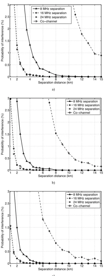
B. Adjacent channel interference
For the same C/(N+I)target = 20 dB, other simulations were
conducted to identify exclusion areas depending on the spectral separation between incumbent PWMS and TVWS UE. The frequency of operation for the PWMS system is maintained at 658 MHz, while TVWS UE frequency of operation is moved away up to three adjacent channels, each with 8 MHz bandwidth, according to the DVB-T channel grid. Results are plotted in Fig. 6 for scenario 1 to 3. Co-channel
results are also included for comparison. Exclusion areas can be considerably reduced when increasing the spectral separation between TVWS UE and PWMS systems. However, and for all scenarios, no further improvements are visible by increasing the channel gap above 16 MHz.
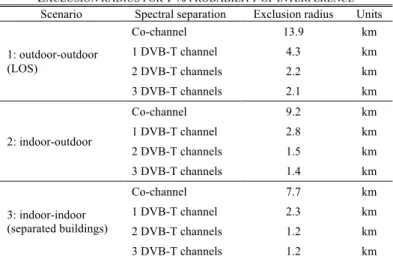
Table IV gives a summary of the protection distance for 1% probability of interference, for all scenarios with co-channel and adjacent-channel interference. The results show that protection distances between PWMS system and secondary users depend on the scenario and the spectral separation. Co-channel interference is the most limitative scenario, with a strong influence on TVWS availability, due to large protection distance around primary PWMS receivers, varying from 7.7 km to 13.9 km. Increasing the frequency gap between primary and secondary users lowers the protection distance, and hence increases the TVWS area. With 8 MHz gap, corresponding to one DVB-T channel, protection distance varies between 2.3 km and 4.3 km, whereas for 16 MHz gap, corresponding to two DVB-T channels, protection distance decreases between 1.2 km and 2.2 km. Protection distances obtained with a 24 MHz gap are similar to the last ones, with values between 1.2 km and 2.1 km.
Fig. 5. Probability of interference for 3 scenarios with co-channel interference, as a function of the separation distance between TVWS UE and PWMS receiver.
TABLEIV
EXCLUSION RADIUS FOR 1% PROBABILITY OF INTERFERENCE
Scenario Spectral separation Exclusion radius Units 1: outdoor-outdoor (LOS) Co-channel 13.9 km 1 DVB-T channel 4.3 km 2 DVB-T channels 2.2 km 3 DVB-T channels 2.1 km 2: indoor-outdoor Co-channel 9.2 km 1 DVB-T channel 2.8 km 2 DVB-T channels 1.5 km 3 DVB-T channels 1.4 km 3: indoor-indoor (separated buildings) Co-channel 7.7 km 1 DVB-T channel 2.3 km 2 DVB-T channels 1.2 km 3 DVB-T channels 1.2 km 2 4 6 8 10 12 14 15 1 0 10 20 30 40 50 60 70 80 90 100 Separation distance (km) Probability of interference (%) outdoor−outdoor indoor−outdoor indoor−indoor
a)
b)
c)
Fig. 6. Probability of interference as a function of the separation distance between TVWS UE and PWMS receiver for: a) scenario 1, b) scenario 2 and c) scenario 3.
VI. CONCLUSIONS
This paper deals with the analysis of co-channel and adjacent-channel interference from TVWS UE to PWMS receivers in the UHF band, using a simulation tool. The results enable the definition of exclusion areas around primary PWMS system, where transmissions of secondary users of the spectrum are not allowed. This methodology can be used to populate a geo-location database with available frequency and maximum power that a TVWS device could use, to avoid causing interference.
Further extensions of this work will include the study of other interference scenarios, considering the presence of more than one interferer in the vicinity of the primary system, with variable transmitted power. The model presented will be also improved, considering the mobility of the wireless microphone, as in the case of “breaking news” events.
REFERENCES
[1] "ECC Report 24: Technical considerations regarding harmonisation options for the Digital Dividend," CEPT 2008.
[2] "Digital Dividend: Geolocation for Cognitive Access," Ofcom2010. [3] "ECC Report 159: Technical and operational requirements for the
possible operation of cognitive radio systems in the ‘white spaces’ of the frequency band 470-790 MHz," CEPT 2011.
[4] R. Dionísio, P. Marques, and J. Rodriguez, "TV White Spaces Maps Computation through Interference Analysis," in Future Network &
Mobile Summit, Warsaw, Poland, 2011, pp. 1-9.
[5] . SEAMCAT. Available: http://www.seamcat.org
[6] "3GPP TS 36.101 V9.2.0 - E-UTRA; User Equipment (UE) radio transmission and reception," ed: ETSI.
[7] T. S. Rappaport, Wireless Communications - Principles and Practice. New Jersey: Prentice Hall, 1996.
2 4 6 8 10 12 14 1 15 0 0.5 1 1.5 2 2.5 3 Separation distance (km) Probability of interference (%) 8 MHz separation 16 MHz separation 24 MHz separation Co−channel 2 4 6 8 10 12 14 1 15 0 0.5 1 1.5 2 2.5 3 Separation distance (km) Probability of interference (%) 8 MHz separation 16 MHz separation 24 MHz separation Co−channel 2 4 6 8 10 12 14 15 1 0 0.5 1 1.5 2 2.5 3 Separation distance (km) Probability of interference (%) 8 MHz separation 16 MHz separation 24 MHz separation Co−channel