CERN-EP-2017-071 2017/09/07
CMS-SUS-16-035
Search for physics beyond the standard model in events
with two leptons of same sign, missing transverse
momentum, and jets in proton-proton collisions at
√
s
=
13 TeV
The CMS Collaboration
∗Abstract
A data sample of events from proton-proton collisions with two isolated same-sign leptons, missing transverse momentum, and jets is studied in a search for signatures of new physics phenomena by the CMS Collaboration at the LHC. The data corre-spond to an integrated luminosity of 35.9 fb−1, and a center-of-mass energy of 13 TeV. The properties of the events are consistent with expectations from standard model processes, and no excess yield is observed. Exclusion limits at 95% confidence level are set on cross sections for the pair production of gluinos, squarks, and same-sign top quarks, as well as top-quark associated production of a heavy scalar or pseudoscalar boson decaying to top quarks, and on the standard model production of events with four top quarks. The observed lower mass limits are as high as 1500 GeV for gluinos, 830 GeV for bottom squarks. The excluded mass range for heavy (pseudo)scalar bosons is 350–360 (350–410) GeV. Additionally, model-independent limits in several topological regions are provided, allowing for further interpretations of the results. Published in the European Physical Journal C as doi:10.1140/epjc/s10052-017-5079-z.
c
2017 CERN for the benefit of the CMS Collaboration. CC-BY-3.0 license
∗See Appendix A for the list of collaboration members
1 Introduction
Final states with two leptons of same charge, denoted as same-sign (SS) dileptons, are produced rarely by standard model (SM) processes in proton-proton (pp) collisions. Because the SM rates of SS dileptons are low, studies of these final states provide excellent opportunities to search for manifestations of physics beyond the standard model (BSM). Over the last decades, a large number of new physics mechanisms have been proposed to extend the SM and address its shortcomings. Many of these can give rise to potentially large contributions to the SS dilepton signature, e.g., the production of supersymmetric (SUSY) particles [1, 2], SS top quarks [3, 4], scalar gluons (sgluons) [5, 6], heavy scalar bosons of extended Higgs sectors [7, 8], Majorana neutrinos [9], and vector-like quarks [10].
In the SUSY framework [11–20], the SS final state can appear in R-parity conserving models through gluino or squark pair production when the decay of each of the pair-produced particles yields one or more W bosons. For example, a pair of gluinos (which are Majorana particles) can give rise to SS charginos and up to four top quarks, yielding signatures with up to four W bosons, as well as jets, b quark jets, and large missing transverse momentum (Emiss
T ). Similar signatures can also result from the pair production of bottom squarks, subsequently decaying to charginos and top quarks.
While R-parity conserving SUSY models often lead to signatures with large Emiss
T , it is also interesting to study final states without significant Emiss
T beyond what is produced by the neu-trinos from leptonic W boson decays. For example, some SM and BSM scenarios can lead to the production of SS or multiple top quark pairs, such as the associated production of a heavy (pseudo)scalar, which subsequently decays to a pair of top quarks. This scenario is real-ized in Type II two Higgs doublet models (2HDM) where associated production with a single top quark or a tt pair can in some cases provide a promising window to probe these heavy (pseudo)scalar bosons [21–23].
This paper extends the search for new physics presented in Ref. [24]. We consider final states with two leptons (electrons and muons) of same charge, two or more hadronic jets, and mod-erate Emiss
T . Compared to searches with zero or one lepton, this final state provides enhanced sensitivity to low-momentum leptons and SUSY models with compressed mass spectra. The results are based on an integrated luminosity corresponding to 35.9 fb−1of√s=13 TeV proton-proton collisions collected with the CMS detector at the CERN LHC. Previous LHC searches in the SS dilepton channel have been performed by the ATLAS [25–27] and CMS [24, 28–32] Col-laborations. With respect to Ref. [24], the event categorization is extended to take advantage of the increased integrated luminosity, the estimate of rare SM backgrounds is improved, and the (pseudo)scalar boson interpretation is added.
The results of the search are interpreted in a number of specific BSM models discussed in Sec-tion 2. In addiSec-tion, model-independent results are also provided in several kinematic regions to allow for further interpretations. These results are given as a function of hadronic activity and of Emiss
T , as well as in a set of inclusive regions with different topologies. The full analysis results are also summarized in a smaller set of exclusive regions to be used in combination with the background correlation matrix to facilitate their reinterpretation.
2 Background and signal simulation
Monte Carlo (MC) simulations are used to estimate SM background contributions and to es-timate the acceptance of the event selection for BSM models. The MADGRAPH5 aMC@NLO
2.2.2 [33–35] andPOWHEGv2 [36, 37] next-to-leading order (NLO) generators are used to
simu-late almost all SM background processes based on the NNPDF3.0 NLO [38] parton distribution functions (PDFs). New physics signal samples, as well as the same-sign W±W± process, are
generated with MADGRAPH5 aMC@NLOat leading order (LO) precision, with up to two
addi-tional partons in the matrix element calculations, using the NNPDF3.0 LO [38] PDFs. Parton showering and hadronization, as well as the double-parton scattering production of W±W±,
are described using the PYTHIA 8.205 generator [39] with the CUETP8M1 tune [40, 41]. The
GEANT4 package [42] is used to model the CMS detector response for background samples,
while the CMS fast simulation package [43] is used for signal samples.
To improve on the MADGRAPH modeling of the multiplicity of additional jets from
initial-state radiation (ISR), MADGRAPH tt MC events are reweighted based on the number of ISR
jets (NISR
J ), so as to make the light-flavor jet multiplicity in dilepton tt events agree with the one observed in data. The same reweighting procedure is applied to SUSY MC events. The reweighting factors vary between 0.92 and 0.51 for NISR
J between 1 and 6. We take one half of the deviation from unity as the systematic uncertainty in these reweighting factors.
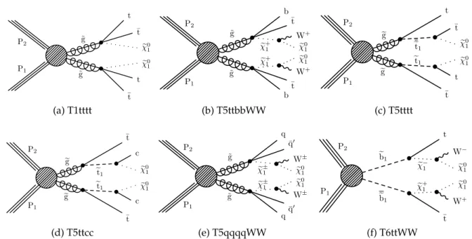
The new physics signal models probed by this search are shown in Figs. 1 and 2. In each of the simplified SUSY models [44, 45] of Fig. 1, only two or three new particles have masses sufficiently low to be produced on-shell, and the branching fraction for the decays shown are assumed to be 100%. Gluino pair production models giving rise to signatures with up to four b quarks and up to four W bosons are shown in Figs. 1a–e. In these models, the gluino decays to the lightest squark (eg → eqq), which in turn decays to same-flavor (eq → qeχ01) or different-flavor (eq→ q0χe±1) quarks. The chargino decays to a W boson and a neutralino (eχ±1 → W±χe01),
where the eχ0
1 escapes detection and is taken to be the lightest SUSY particle (LSP). The first two scenarios considered in Figs. 1a and 1b include an off-shell third-generation squark (et or eb) leading to the three-body decay of the gluino, eg→ tteχ01(T1tttt) and eg→tbeχ+1 (T5ttbbWW), resulting in events with four W bosons and four b quarks. In the T5ttbbWW model, the mass splitting between chargino and neutralino is set to mχe±
1 −mχe01 = 5 GeV, so that two of the
W bosons are produced off-shell and can give rise to low transverse momentum (pT) leptons. The next two models shown (Figs. 1c and d) include an on-shell top squark with different mass splitting between the et and the eχ0
1, and consequently different decay modes: in the T5tttt model the mass splitting is equal to the top quark mass (met−mχe0
1 = mt), favoring the et→teχ
0 1 decay, while in the T5ttcc model the mass splitting is only 20 GeV, favoring the flavor changing neutral current et → ceχ01 decay. In Fig. 1e, the decay proceeds through a virtual light-flavor squark, leading to a three-body decay to eg → qq0χe1±, resulting in a signature with two W
bosons and four light-flavor jets. The two W bosons can have the same charge, giving rise to SS dileptons. This model, T5qqqqWW, is studied as a function of the gluino and eχ0
1mass, with two different assumptions for the chargino mass: mχe±
1 =0.5(meg+mχe01), producing mostly on-shell
W bosons, and mχe±
1 = mχe01 +20 GeV, producing off-shell W bosons. Finally, Fig. 1f shows a
model of bottom squark production followed by the eb→teχ±1 decay, resulting in two b quarks and four W bosons. This model, T6ttWW, is studied as a function of the eb and eχ±
1 masses, keeping the eχ0
1mass at 50 GeV, resulting in two of the W bosons being produced off-shell when the eχ±
1 and eχ01masses are close. The production cross sections for SUSY models are calculated at NLO plus next-to-leading logarithmic (NLL) accuracy [46–51].
The processes shown in Fig. 2, ttH, tHq, and tWH, represent the top quark associated produc-tion of a scalar (H) or a pseudoscalar (A). The subsequent decay of the (pseudo)scalar to a pair of top quarks then gives rise to final states including a total of three or four top quarks. For the purpose of interpretation, we use LO cross sections for the production of a heavy Higgs boson
P1 P2 g g ¯t t 0 1 0 1 ¯t t ˜ ˜ T1ttt (a) T1tttt P1 P2 ˜ g ˜ g e+ 1 e+ 1 b ¯t W+ e0 1 e0 1 W+ ¯t b (b) T5ttbbWW P1 P2 eg eg et1 et1 ¯t t e0 1 e0 1 ¯t t (c) T5tttt P1 P2 eg eg et1 et1 ¯t c e0 1 e0 1 c ¯t (d) T5ttcc P1 P2 ˜ g ˜ g e± 1 e± 1 q¯q W± e0 1 e0 1 W± ¯ q q (e) T5qqqqWW P1 P2 eb1 eb1 e+ 1 e1 ¯t W+ e0 1 e0 1 W t (f) T6ttWW
Figure 1: Diagrams illustrating the simplified SUSY models considered in this analysis. P1 P2 g g ¯t t 0 1 0 1 ¯t t ˜ ˜ T1ttt (a) T1tttt P1 P2 ˜ g ˜ g e+ 1 e+ 1 b ¯t W+ e0 1 e0 1 W+ ¯t b (b) T5ttbbWW P1 P2 eg eg et1 et1 ¯t t e0 1 e0 1 ¯t t (c) T5tttt P1 P2 eg eg et1 et1 ¯t c e0 1 e0 1 c ¯t (d) T5ttcc P1 P2 ˜ g ˜ g e± 1 e± 1 q¯q W± e0 1 e0 1 W± ¯ q q (e) T5qqqqWW P1 P2 eb1 eb1 e+ 1 e1 ¯t W+ e0 1 e0 1 W t (f) T6ttWW
Figure 1: Diagrams illustrating the simplified SUSY models considered in this analysis.
g g ¯t t t ¯t H(A) (a) t¯tH W b ¯ q q¯ t t ¯t H(A) (b) tHq b g H(A) t W tt ¯t (c) tHW
Figure 2: Diagrams for scalar (pseudoscalar) production in association with top quarks.
3
The CMS detector and event reconstruction
The central feature of the CMS detector is a superconducting solenoid of 6 m internal diameter, providing a magnetic field of 3.8 T. Within the solenoid volume are a silicon pixel and strip tracker, a lead tungstate crystal electromagnetic calorimeter (ECAL), and a brass and scintillator hadron calorimeter (HCAL), each composed of a barrel and two endcap sections. Forward calorimeters extend the pseudorapidity coverage provided by the barrel and endcap detectors. Muons are measured in gas-ionization detectors embedded in the steel flux-return yoke outside the solenoid. A more detailed description of the CMS detector, together with a definition of the coordinate system used and the relevant kinematic variables, can be found in Ref. [49].
Events of interest are selected using a two-tiered trigger system [50]. The first level (L1), com-posed of custom hardware processors, uses information from the calorimeters and muon de-tectors to select events at a rate of around 100 kHz within a time interval of less than 4 µs. The second level, known as the high-level trigger (HLT), consists of a farm of processors running a version of the full event reconstruction software optimized for fast processing, and reduces the event rate to less than 1 kHz before data storage.
Events are processed using the particle-flow (PF) algorithm [51, 52], which reconstructs and identifies each individual particle with an optimized combination of information from the various elements of the CMS detector. The energy of photons is directly obtained from the ECAL measurement. The energy of electrons is determined from a combination of the elec-Figure 2: Diagrams for scalar (pseudoscalar) boson production in association with top quarks. in the context of the Type II 2HDM of Ref. [23]. The mass of the new particle is varied in the range [350, 550] GeV, where the lower mass boundary is chosen in such a way as to allow the decay of the (pseudo)scalar into on-shell top quarks.
3
The CMS detector and event reconstruction
The central feature of the CMS detector is a superconducting solenoid of 6 m internal diameter, providing a magnetic field of 3.8 T. Within the solenoid volume are a silicon pixel and strip tracker, a lead tungstate crystal electromagnetic calorimeter (ECAL), and a brass and scintilla-tor hadron calorimeter (HCAL), each composed of a barrel and two endcap sections. Forward calorimeters extend the pseudorapidity (η) coverage provided by the barrel and endcap detec-tors. Muons are measured in gas-ionization detectors embedded in the steel flux-return yoke outside the solenoid. A more detailed description of the CMS detector, together with a def-inition of the coordinate system used and the relevant kinematic variables, can be found in Ref. [52].
Events of interest are selected using a two-tiered trigger system [53]. The first level (L1), com-posed of custom hardware processors, uses information from the calorimeters and muon de-tectors to select events at a rate of around 100 kHz within a time interval of less than 4 µs. The second level, known as the high-level trigger (HLT), consists of a farm of processors running a
version of the full event reconstruction software optimized for fast processing, and reduces the event rate to less than 1 kHz before data storage.
Events are processed using the particle-flow (PF) algorithm [54, 55], which reconstructs and identifies each individual particle with an optimized combination of information from the various elements of the CMS detector. The energy of photons is directly obtained from the ECAL measurement. The energy of electrons is determined from a combination of the elec-tron momentum at the primary interaction vertex as determined by the tracker, the energy of the corresponding ECAL cluster, and the energy sum of all bremsstrahlung photons spatially compatible with the electron track [56]. The energy of muons is obtained from the curvature of the corresponding track, combining information from the silicon tracker and the muon sys-tem [57]. The energy of charged hadrons is determined from a combination of their momen-tum measured in the tracker and the matching ECAL and HCAL energy deposits, corrected for the response function of the calorimeters to hadronic showers. Finally, the energy of neutral hadrons is obtained from the corresponding corrected ECAL and HCAL energy.
Hadronic jets are clustered from neutral PF candidates and charged PF candidates associ-ated with the primary vertex, using the anti-kT algorithm [58, 59] with a distance parameter R = √(∆η)2+ (∆φ)2of 0.4. Jet momentum is determined as the vectorial sum of all PF can-didate momenta in the jet. An offset correction is applied to jet energies to take into account the contribution from additional proton-proton interactions (pileup) within the same or nearby bunch crossings. Jet energy corrections are derived from simulation, and are improved with in situ measurements of the energy balance in dijet and photon+jet events [60, 61]. Additional selection criteria are applied to each event to remove spurious jet-like features originating from isolated noise patterns in certain HCAL regions. Jets originating from b quarks are identi-fied (b tagged) using the medium working point of the combined secondary vertex algorithm CSVv2 [62]. The missing transverse momentum vector~pTmiss is defined as the projection on the plane perpendicular to the beams of the negative vector sum of the momenta of all recon-structed PF candidates in an event [63]. Its magnitude is referred to as Emiss
T . The sum of the transverse momenta of all jets in an event is referred to as HT.
4 Event selection and search strategy
The event selection and the definition of the signal regions (SRs) follow closely the analysis strategy established in Ref. [24]. With respect to the previous search, the general strategy has remained unchanged. We target, in a generic way, new physics signatures that result in SS dileptons, hadronic activity, and Emiss
T , by subdividing the event sample into several SRs sensi-tive to a variety of new physics models. The number of SRs was increased to take advantage of the larger integrated luminosity. Table 1 summarizes the basic kinematic requirements for jets and leptons (further details, including the lepton identification and isolation requirements, can be found in Ref. [24]).
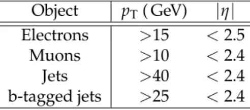
Table 1: Kinematic requirements for leptons and jets. Note that the pT thresholds to count jets and b-tagged jets are different.
Object pT( GeV) |η| Electrons >15 <2.5
Muons >10 <2.4
Jets >40 <2.4
Events are selected using triggers based on two sets of HLT algorithms, one simply requiring two leptons, and one additionally requiring HT >300 GeV. The HTrequirement allows for the lepton isolation requirement to be removed and for the lepton pTthresholds to be set to 8 GeV for both leptons, while in the pure dilepton trigger the leading and subleading leptons are required to have pT > 23(17)GeV and pT > 12 (8)GeV, respectively, for electrons (muons). Based on these trigger requirements, leptons are classified as high (pT > 25 GeV) and low (10< pT <25 GeV) momentum, and three analysis regions are defined: high (HH), high-low (HL), and high-low-high-low (LL).
The baseline selection used in this analysis requires at least one SS lepton pair with an invari-ant mass above 8 GeV, at least two jets, and Emiss
T >50 GeV. To reduce Drell–Yan backgrounds, events are rejected if an additional loose lepton forms an opposite-sign same-flavor pair with one of the two SS leptons, with an invariant mass less than 12 GeV or between 76 and 106 GeV. Events passing the baseline selection are then divided into SRs to separate the different back-ground processes and to maximize the sensitivity to signatures with different jet multiplicity (Njets), flavor (Nb), visible and invisible energy (HT and ETmiss), and lepton momentum spectra (the HH/HL/LL categories mentioned previously). The mmin
T variable is defined as the small-est of the transverse masses constructed between~pTmiss and each of the leptons. This variable features a cutoff near the W boson mass for processes with only one prompt lepton, so it is used to create SRs where the nonprompt lepton background is negligible. To further improve sensitivity, several regions are split according to the charge of the leptons (++or−−), taking advantage of the charge asymmetry of SM backgrounds, such as ttW or WZ, with a single W boson produced in pp collisions. Only signal regions dominated by such backgrounds and with a sufficient predicted yield are split by charge. In the HH and HL categories, events in the tail regions HT > 1125 GeV or EmissT > 300 GeV are inclusive in Njets, Nb, and mminT in or-der to ensure a reasonable yield of events in these SRs. The exclusive SRs resulting from this classification are defined in Tables 2–4.
The lepton reconstruction and identification efficiency is in the range of 45–70% (70–90%) for electrons (muons) with pT > 25 GeV, increasing as a function of pT and converging to the maximum value for pT > 60 GeV. In the low-momentum regime, 15 < pT < 25 GeV for electrons and 10 < pT < 25 GeV for muons, the efficiencies are 40% for electrons and 55% for muons. The lepton trigger efficiency for electrons is in the range of 90-98%, converging to the maximum value for pT > 30 GeV, and around 92% for muons. The chosen b tagging working point results in approximately a 70% efficiency for tagging a b quark jet and a<1% mistagging rate for light-flavor jets in tt events [62]. The efficiencies of the HT and EmissT requirements are mostly determined by the jet energy and Emiss
T resolutions, which are discussed in Refs. [60, 61, 64].
5 Backgrounds
Standard model background contributions arise from three sources: processes with prompt SS dileptons, mostly relevant in regions with high Emiss
T or HT; events with a nonprompt lepton, dominating the overall final state; and opposite-sign dilepton events with a charge-misidentified lepton, the smallest contribution. In this paper we use the shorthand “nonprompt leptons” to refer to electrons or muons from the decays of heavy- or light-flavor hadrons, hadrons misidentified as leptons, or electrons from conversions of photons in jets.
Several categories of SM processes that result in the production of electroweak bosons can give rise to an SS dilepton final state. These include production of multiple bosons in the same event (prompt photons, W, Z, and Higgs bosons), as well as single-boson production
Table 2: Signal region definitions for the HH selection. Regions split by charge are indicated with (++) and (−−).
Nb mminT (GeV) EmissT (GeV) Njets HT<300 GeV HT∈ [300, 1125]GeV HT∈ [1125, 1300]GeV HT∈ [1300, 1600]GeV HT>1600 GeV
0 <120 50−200 2-4 SR1 SR2 SR46 (++) / SR47 (−−) SR48 (SR49 (++−−) /) SR50 (SR51 (++−−) /) ≥5 SR3 SR4 200−300 2-4≥5 SR5 (++) / SR6 (SR7 −−) >120 50 −200 2-4≥5 SR8 (++) / SR9 (−−) SR10 200−300 2-4≥5 1 <120 50 −200 2-4≥5 SR11 SR12 SR13 (++) / SR14 (−−) SR15 (++) / SR16 (−−) 200−300 2-4 SR17 (++) / SR18 (−−) ≥5 SR19 >120 50−200 2-4 SR20 (++) / SR21 (−−) ≥5 SR22 200−300 2-4 ≥5 2 <120 50−200 2-4 SR23 SR24 ≥5 SR25 (++) / SR26 (−−) SR27 (++) / SR28 (−−) 200−300 2-4 SR29 (++) / SR30 (−−) ≥5 SR31 >120 50−200 2-4 SR32 (++) / SR33 (−−) ≥5 SR34 200−300 2-4≥5 ≥3 <120 20050−−200300 ≥2 SR35 (SR36 (−−++) /) SR37 (++SR39) / SR38 (−−) >120 50−300 ≥2 SR40 SR41 inclusive inclusive 300>−500500 ≥2 —— SR44 (SR42 (++++) / SR45 () / SR43 (−−−−))
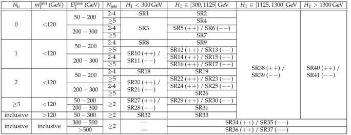
Table 3: Signal region definitions for the HL selection. Regions split by charge are indicated with (++) and (−−).
Nb mminT (GeV) EmissT (GeV) Njets HT<300 GeV HT∈ [300, 1125] GeV HT∈ [1125, 1300] GeV HT>1300 GeV
0 <120 50 − 200 2-4 SR1 SR2 SR38 (++) / SR39 (−−) SR40 (++) /SR41 (−−) ≥5 SR3 SR4 200 − 300 2-4≥5 SR5 (++) / SR6 (−−)SR7 1 <120 50 − 200 2-4 SR8 SR9 ≥5 SR10 (++) / SR11 (−−) SR12 (++) / SR13 (−−) 200 − 300 2-4≥5 SR14 (++) / SR15 (−−)SR16 (++) / SR17 (−−) 2 <120 50 − 200 2-4 SR18 SR19 ≥5 SR20 (++) / SR21 (−−) SR22 (++) / SR23 (−−) 200 − 300 2-4≥5 SR24 (++) / SR25 (−−)SR26 ≥3 <120 200 − 30050 − 200 ≥2 SR27 (++) /SR28 (−−) SR29 (++) / SR30 (−−)SR31 inclusive >120 50 − 300 ≥2 SR32 SR33 inclusive inclusive 300 − 500>500 ≥2 —— SR34 (++) / SR35 (−−)SR36 (++) / SR37 (−−)
in association with top quarks. Among these SM processes, the dominant ones are WZ, ttW, and ttZ production, followed by the W±W±process. The remaining SM processes are grouped
into two categories, “Rare” (including ZZ, WWZ, WZZ, ZZZ, tWZ, tZq, as well as tttt and double parton scattering) and “X+γ” (including Wγ, Zγ, ttγ, and tγ). The expected yields from these SM backgrounds are estimated from simulation, accounting for both the theoretical and experimental uncertainties discussed in Section 6.
For the WZ and ttZ backgrounds, a three-lepton (3L) control region in data is used to scale the simulation, based on a template fit to the distribution of the number of b jets. The 3L control region requires at least two jets, Emiss
T > 30 GeV, and three leptons, two of which must form an opposite-sign same-flavor pair with an invariant mass within 15 GeV of the Z boson mass. In the fit to data, the normalization and shapes of all the components are allowed to vary
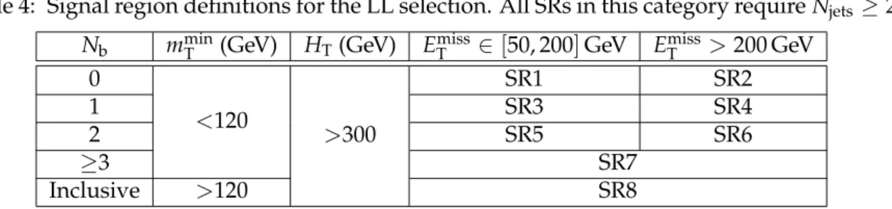
Table 4: Signal region definitions for the LL selection. All SRs in this category require Njets ≥2. Nb mminT (GeV) HT(GeV) EmissT ∈ [50, 200]GeV EmissT >200 GeV
0 <120 >300 SR1 SR2 1 SR3 SR4 2 SR5 SR6 ≥3 SR7 Inclusive >120 SR8
according to experimental and theoretical uncertainties. The scale factors obtained from the fit in the phase space of the 3L control region are 1.26±0.09 for the WZ process, and 1.14±0.30 for the ttZ process.
The nonprompt lepton background, which is largest for regions with low mmin
T and low HT, is estimated by the “tight-to-loose” method, which was employed in several previous versions of the analysis [28–32], and significantly improved in the latest version [24] to account for the kinematics and flavor of the parent parton of the nonprompt lepton. The tight-to-loose method uses two control regions, the measurement region and the application region. The measument region consists of a sample of single-lepton events enriched in nonprompt leptons by re-quirements on Emiss
T and transverse mass that suppress the W→ `νcontribution. This sample is used to extract the probability for a nonprompt lepton that satisfies the loose selection to also satisfy the tight selection. This probability (eTL) is calculated as a function of lepton pcorrT (de-fined below) and η, separately for electrons and muons, and separately for lepton triggers with and without an isolation requirement. The application region is a SS dilepton region where both of the leptons satisfy the loose selection but at least one of them fails the tight selection. This region is subsequently divided into a set of subregions with the exact same kinematic re-quirements as those in the SRs. Events in the subregions are weighted by a factor eTL/(1−eTL) for each lepton in the event failing the tight requirement. The nonprompt background in each SR is then estimated as the sum of the event weights in the corresponding subregion. The pcorr
T parametrization, where pcorr
T is defined as the lepton pT plus the energy in the isolation cone exceeding the isolation threshold value, is chosen because of its correlation with the parent parton pT, improving the stability of the eTLvalues with respect to the sample kinematics. To improve the stability of the eTLvalues with respect to the flavor of the parent parton, the loose electron selection is adopted. This selection increases the number of nonprompt electrons from the fragmentation and decay of light-flavor partons, resulting in eTL values similar to those from heavy-flavor parent partons.
The prediction from the tight-to-loose method is cross-checked using an alternative method based on the same principle, similar to that described in Ref. [65]. In this cross-check, which aims to remove kinematic differences between measurement and application regions, the mea-surement region is obtained from SS dilepton events where one of the leptons fails the impact parameter requirement. With respect to the nominal method, the loose lepton definition is adapted to reduce the effect of the correlation between isolation and impact parameter. The predictions of the two methods are found to be consistent within systematic uncertainties. Charge misidentification of electrons is a small background that can arise from severe brems-strahlung in the tracker material. Simulation-based studies with tight leptons indicate that the muon charge misidentification probability is negligible, while for electrons it ranges be-tween 10−5and 10−3. The charge misidentification background is estimated from data using an opposite-sign control region for each SS SR, scaling the control region yield by the charge misidentification probability measured in simulation. A low-Emiss
pairs in the Z boson mass window, is used to cross-check the MC prediction for the misidenti-fication probability, both inclusively and — where the number of events in data allows it — as a function of electron pTand η.
6 Systematic uncertainties
Several sources of systematic uncertainty affect the predicted yields for signal and background processes, as summarized in Table 5. Experimental uncertainties are based on measurements in data of the trigger efficiency, the lepton identification efficiency, the b tagging efficiency [62], the jet energy scale, and the integrated luminosity [66], as well as on the inelastic cross section value affecting the pileup rate. Theoretical uncertainties related to unknown higher-order effects are estimated by varying simultaneously the factorization and renormalization scales by a factor of two, while uncertainties in the PDFs are obtained using replicas of the NNPDF3.0 set [38]. Experimental and theoretical uncertainties affect both the overall yield (normalization) and the relative population (shape) across SRs, and they are taken into account for all signal samples as well as for the samples used to estimate the main prompt SS dilepton backgrounds: WZ, ttW, ttZ, W±W±. For the WZ and ttZ backgrounds, the control region fit results are used for
the normalization, so these uncertainties are only taken into account for the shape of the back-grounds. For the smallest background samples, Rare and X+γ, a 50% uncertainty is assigned in place of the scale and PDF variations.
The normalization and the shapes of the nonprompt lepton and charge misidentification back-grounds are estimated from control regions in data. In addition to the statistical uncertainties from the control region yields, dedicated systematic uncertainties are associated with the meth-ods used in this estimate. For the nonprompt lepton background, a 30% uncertainty (increased to 60% for electrons with pT >50 GeV) accounts for the performance of the method in simula-tion and for the differences in the two alternative methods described in Secsimula-tion 5. In addisimula-tion, the uncertainty in the prompt lepton yield in the measurement region, relevant when estimat-ing eTLfor high-pTleptons, results in a 1–30% effect on the estimate. For the charge misidenti-fication background, a 20% uncertainty is assigned to account for possible mismodeling of the charge misidentification rate in simulation.
7 Results and interpretation
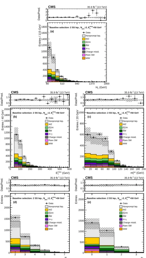
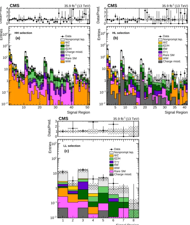
A comparison between observed yields and the SM background prediction is shown in Fig. 3 for the kinematic variables used to define the analysis SRs: HT, EmissT , mminT , Njets, and Nb. The distributions are shown after the baseline selection defined in Section 4. The full results of the search in each SR are shown in Fig. 4 and Table 6. The SM predictions are generally consistent with the data. The largest deviations are seen in HL SR 36 and 38, with a local significance, taking these regions individually or combining them with other regions adjacent in phase space, that does not exceed 2 standard deviations.
These results are used to probe the signal models discussed in Section 2: simplified SUSY mod-els, (pseudo)scalar boson production, four top quark production, and SS top quark production. We also interpret the results as model-independent limits as a function of HT and EmissT . With the exception of the new (pseudo)scalar boson limits, the results can be compared to the pre-vious version of the analysis [24], showing significant improvements due to the increase in the integrated luminosity and the optimization of SR definitions.
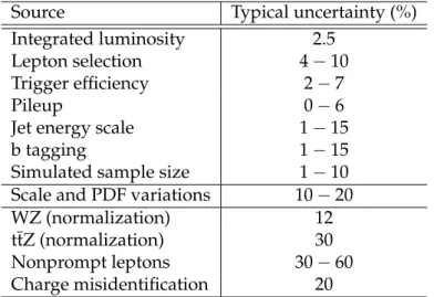
Table 5: Summary of the sources of uncertainty and their effect on the yields of different pro-cesses in the SRs. The first two groups list experimental and theoretical uncertainties assigned to processes estimated using simulation, while the last group lists uncertainties assigned to processes whose yield is estimated from data. The uncertainties in the first group also apply to signal samples. Reported values are representative for the most relevant signal regions.
Source Typical uncertainty (%)
Integrated luminosity 2.5
Lepton selection 4−10
Trigger efficiency 2−7
Pileup 0−6
Jet energy scale 1−15
b tagging 1−15
Simulated sample size 1−10
Scale and PDF variations 10−20
WZ (normalization) 12
ttZ (normalization) 30
Nonprompt leptons 30−60
Charge misidentification 20
signal and background uncertainties and their correlations — are combined using an asymp-totic formulation of the modified frequentist CLs criterion [67–70]. When testing a model, all new particles not included in the specific model are considered too heavy to take part in the interaction. To convert cross section limits into mass limits, the signal cross sections specified in Section 2 are used.
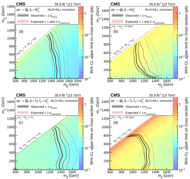
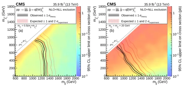
The observed SUSY cross section limits as a function of the gluino and LSP masses, as well as the observed and expected mass limits for each simplified model, are shown in Fig. 5 for gluino pair production models with each gluino decaying through a chain containing off- or on-shell third-generation squarks. These models, which result in signatures with two or more b quarks and two or more W bosons in the final state, are introduced in Section 2 as T1tttt, T5ttbbWW, T5tttt, and T5ttcc. Figure 6 shows the limits for a model of gluino production followed by a decay through off-shell first- or second-generation squarks and a chargino. Two different assumptions are made on the chargino mass, taken to be between that of the gluino and the LSP. These T5qqqqWW models result in no b quarks and either on-shell or off-shell W bosons. Bottom squark pair production followed by a decay through a chargino, T6ttWW, resulting in two b quarks and four W bosons, is shown in Fig. 7. For all of the models probed, the observed limit agrees well with the expected one, extending the reach of the previous analysis by 200–300 GeV and reaching 1.5, 1.1, and 0.83 TeV for gluino, LSP, and bottom squark masses, respectively.
The observed and expected cross section limits on the production of a heavy scalar or a pseu-doscalar boson in association with one or two top quarks, followed by its decay to top quarks, are shown in Fig. 8. The limits are compared with the total cross section of the processes de-scribed in Section 2. The observed limit, which agrees well with the expected one, excludes scalar (pseudoscalar) masses up to 360 (410) GeV.
The SM four top quark production, pp → tttt, is normally included among the rare SM back-grounds. When treating this process as signal, its observed (expected) cross section limit is determined to be 42 (27+13
−8 ) fb at 95% CL, to be compared to the SM expectation of 9.2+−2.92.4fb [33]. This is a significant improvement with respect to the observed (expected) limits obtained
Data/MC 0 1 2 3 4 Data/Pred. (13 TeV) -1 35.9 fb CMS (GeV) T H 80 510 940 1370 1800 Entries / 115 GeV 0 200 400 600 800 1000 1200 1400 1600 1800 Data Nonprompt lep. WZ Z/H t t W t t γ X+ Charge misid. Rare SM WW >50 GeV miss T 2, E ≥ jets
Baseline selection: 2 SS lep., N (a) Data/MC 0 0.5 1 1.5 2 Data/Pred. (13 TeV) -1 35.9 fb CMS (GeV) miss T E 0 100 200 300 400 500 600 Entries / 40 GeV 0 200 400 600 800 1000 1200 1400 1600 1800 2000 Data Nonprompt lep. WZ Z/H t t W t t γ X+ Charge misid. Rare SM WW >50 GeV miss T 2, E ≥ jets
Baseline selection: 2 SS lep., N (b) Data/MC 0 0.5 1 1.5 2 Data/Pred. (13 TeV) -1 35.9 fb CMS (GeV) min T m 0 20 40 60 80 100 120 140 160 180 200 Entries / 20 GeV 0 200 400 600 800 1000 Data Nonprompt lep. WZ Z/H t t W t t γ X+ Charge misid. Rare SM WW >50 GeV miss T 2, E ≥ jets
Baseline selection: 2 SS lep., N (c) Data/MC 0 0.5 1 1.5 2 Data/Pred. (13 TeV) -1 35.9 fb CMS jets N 2 3 4 5 6 7 Entries 0 500 1000 1500 2000 2500 Data Nonprompt lep. WZ Z/H t t W t t γ X+ Charge misid. Rare SM WW >50 GeV miss T 2, E ≥ jets
Baseline selection: 2 SS lep., N (d) Data/MC 0 0.5 1 1.5 2 Data/Pred. (13 TeV) -1 35.9 fb CMS b N 0 1 2 3 Entries 0 500 1000 1500 2000 2500 Data Nonprompt lep. WZ Z/H t t W t t γ X+ Charge misid. Rare SM WW >50 GeV miss T 2, E ≥ jets
Baseline selection: 2 SS lep., N (e)
Figure 3: Distributions of the main analysis variables: HT (a), ETmiss(b), mminT (c), Njets (d), and Nb(e), after the baseline selection requiring a pair of SS leptons, two jets, and EmissT >50 GeV. The last bin includes the overflow events and the hatched area represents the total uncertainty in the background prediction. The upper panels show the ratio of the observed event yield to the background prediction.
Data/MC 0 1 2 3 4 Data/Pred. (13 TeV) -1 35.9 fb CMS Signal Region 10 20 30 40 50 Entries 2 − 10 1 − 10 1 10 2 10 3 10 4 10 Data Nonprompt lep. WZ W t t Z/H t t Charge misid. γ X+ Rare SM WW HH selection (a) Data/MC 0 1 2 3 4 Data/Pred. (13 TeV) -1 35.9 fb CMS Signal Region 5 10 15 20 25 30 35 40 Entries 2 − 10 1 − 10 1 10 2 10 3 10 4 10 Data Nonprompt lep. WZ Z/H t t W t t γ X+ Rare SM WW Charge misid. HL selection (b) Data/MC 0 1 2 3 Data/Pred. (13 TeV) -1 35.9 fb CMS Signal Region 1 2 3 4 5 6 7 8 Entries 2 − 10 1 − 10 1 10 2 10 3 10 Data Nonprompt lep. WZ Z/H t t γ X+ W t t WW Rare SM Charge misid. LL selection (c)
Figure 4: Event yields in the HH (a), HL (b), and LL (c) signal regions. The hatched area represents the total uncertainty in the background prediction. The upper panels show the ratio of the observed event yield to the background prediction.
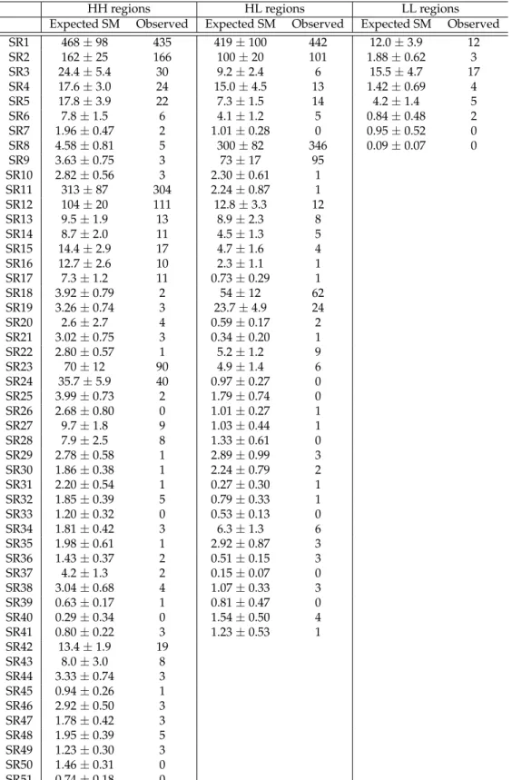
Table 6: Number of expected background and observed events in different SRs in this analysis.
HH regions HL regions LL regions
Expected SM Observed Expected SM Observed Expected SM Observed
SR1 468±98 435 419±100 442 12.0±3.9 12 SR2 162±25 166 100±20 101 1.88±0.62 3 SR3 24.4±5.4 30 9.2±2.4 6 15.5±4.7 17 SR4 17.6±3.0 24 15.0±4.5 13 1.42±0.69 4 SR5 17.8±3.9 22 7.3±1.5 14 4.2±1.4 5 SR6 7.8±1.5 6 4.1±1.2 5 0.84±0.48 2 SR7 1.96±0.47 2 1.01±0.28 0 0.95±0.52 0 SR8 4.58±0.81 5 300±82 346 0.09±0.07 0 SR9 3.63±0.75 3 73±17 95 SR10 2.82±0.56 3 2.30±0.61 1 SR11 313±87 304 2.24±0.87 1 SR12 104±20 111 12.8±3.3 12 SR13 9.5±1.9 13 8.9±2.3 8 SR14 8.7±2.0 11 4.5±1.3 5 SR15 14.4±2.9 17 4.7±1.6 4 SR16 12.7±2.6 10 2.3±1.1 1 SR17 7.3±1.2 11 0.73±0.29 1 SR18 3.92±0.79 2 54±12 62 SR19 3.26±0.74 3 23.7±4.9 24 SR20 2.6±2.7 4 0.59±0.17 2 SR21 3.02±0.75 3 0.34±0.20 1 SR22 2.80±0.57 1 5.2±1.2 9 SR23 70±12 90 4.9±1.4 6 SR24 35.7±5.9 40 0.97±0.27 0 SR25 3.99±0.73 2 1.79±0.74 0 SR26 2.68±0.80 0 1.01±0.27 1 SR27 9.7±1.8 9 1.03±0.44 1 SR28 7.9±2.5 8 1.33±0.61 0 SR29 2.78±0.58 1 2.89±0.99 3 SR30 1.86±0.38 1 2.24±0.79 2 SR31 2.20±0.54 1 0.27±0.30 1 SR32 1.85±0.39 5 0.79±0.33 1 SR33 1.20±0.32 0 0.53±0.13 0 SR34 1.81±0.42 3 6.3±1.3 6 SR35 1.98±0.61 1 2.92±0.87 3 SR36 1.43±0.37 2 0.51±0.15 3 SR37 4.2±1.3 2 0.15±0.07 0 SR38 3.04±0.68 4 1.07±0.33 3 SR39 0.63±0.17 1 0.81±0.47 0 SR40 0.29±0.34 0 1.54±0.50 4 SR41 0.80±0.22 3 1.23±0.53 1 SR42 13.4±1.9 19 SR43 8.0±3.0 8 SR44 3.33±0.74 3 SR45 0.94±0.26 1 SR46 2.92±0.50 3 SR47 1.78±0.42 3 SR48 1.95±0.39 5 SR49 1.23±0.30 3 SR50 1.46±0.31 0 SR51 0.74±0.18 0
(GeV) g ~ m 600 800 1000 1200 1400 1600 1800 2000 (GeV)0χ∼1 m 0 200 400 600 800 1000 1200 1400 1600 1800
95% CL upper limit on cross section (pb)
3 − 10 2 − 10 1 − 10 1 ) b + m W (m ⋅ = 2 0 1 χ ∼ -m g ~ m (13 TeV) -1 35.9 fb CMS (a) NLO+NLL exclusion 1 0 χ∼ t t → g ~ , g ~ g ~ → pp theory σ 1 ± Observed experiment σ 1 and 2 ± Expected (GeV) g ~ m 600 800 1000 1200 1400 1600 (GeV) 0χ∼1 m 0 200 400 600 800 1000 1200 1400 1600
95% CL upper limit on cross section (pb)
3 − 10 2 − 10 1 − 10 1 ) b + m W (m ⋅ = 2 0 1 χ ∼ -m g ~ m (13 TeV) -1 35.9 fb CMS + 5 GeV 1 0 χ∼ = m 1 ± χ∼ m (b) NLO+NLL exclusion 1 ± χ∼ tb → g ~ , g ~ g ~ → pp theory σ 1 ± Observed experiment σ 1 and 2 ± Expected (GeV) g ~ m 600 800 1000 1200 1400 1600 (GeV)0χ∼1 m 0 200 400 600 800 1000 1200 1400 1600
95% CL upper limit on cross section (pb)
3 − 10 2 − 10 1 − 10 1 b + m W + m t = m 1 0 χ ∼ - m g ~ m (13 TeV) -1 35.9 fb CMS t + m 1 0 χ∼ = m 1 t ~ m (c) NLO+NLL exclusion 1 0 χ∼ t → 1 t ~ , t 1 t ~ → g ~ , g ~ g ~ → pp theory σ 1 ± Observed experiment σ 1 ± Expected (GeV) g ~ m 600 800 1000 1200 1400 1600 (GeV) ±χ∼1 m 0 200 400 600 800 1000 1200 1400 1600
95% CL upper limit on cross section (pb)
3 − 10 2 − 10 1 − 10 1 b + m W = m 1 0 χ ∼ - m g ~ m (13 TeV) -1 35.9 fb CMS + 20 GeV 1 0 χ∼ = m 1 t ~ m (d) NLO+NLL exclusion 1 0 χ∼ c → 1 t ~ , t 1 t ~ → g ~ , g ~ g ~ → pp theory σ 1 ± Observed experiment σ 1 ± Expected
Figure 5: Exclusion regions at 95% CL in the mχe0
1 versus meg plane for the T1tttt (a) and
T5ttbbWW (b) models, with off-shell third-generation squarks, and the T5tttt (c) and T5ttcc (d) models, with on-shell third-generation squarks. For the T5ttbbWW model, mχe±
1 =mχe01+5 GeV,
for the T5tttt model, met−mχe0
1 = mt, and for the T5ttcc model, met−mχe01 =20 GeV and the decay
proceeds through et→ceχ01. The right-hand side color scale indicates the excluded cross section values for a given point in the SUSY particle mass plane. The solid, black curves represent the observed exclusion limits assuming the NLO+NLL cross sections [46–51] (thick line), or their variations of ±1 standard deviation (thin lines). The dashed, red curves show the expected limits with the corresponding±1 and±2 standard deviation experimental uncertainties. Ex-cluded regions are to the left and below the limit curves.
(GeV) g ~ m 600 800 1000 1200 1400 1600 1800 2000 (GeV)0χ∼1 m 0 200 400 600 800 1000 1200 1400 1600 1800
95% CL upper limit on cross section (pb)
3 − 10 2 − 10 1 − 10 1 0 1 χ ∼ = m g ~ m (13 TeV) -1 35.9 fb CMS ) 1 0 χ∼ +m g ~ = 0.5(m 1 ± χ∼ m (a) NLO+NLL exclusion 1 0 χ∼ 'W q q → g ~ , g ~ g ~ → pp theory σ 1 ± Observed experiment σ 1 and 2 ± Expected (GeV) g ~ m 600 800 1000 1200 1400 1600 1800 2000 (GeV) 0χ∼1 m 0 200 400 600 800 1000 1200 1400 1600 1800
95% CL upper limit on cross section (pb)
3 − 10 2 − 10 1 − 10 1 0 1 χ ∼ = m g ~ m (13 TeV) -1 35.9 fb CMS + 20 GeV 1 0 χ∼ = m 1 ± χ∼ m (b) NLO+NLL exclusion 1 0 χ∼ 'W* q q → g ~ , g ~ g ~ → pp theory σ 1 ± Observed experiment σ 1 and 2 ± Expected
Figure 6: Exclusion regions at 95% CL in the plane of mχe0
1 versus megfor the T5qqqqWW model
with mχe±
1 =0.5(meg+mχe01)(a) and with mχe1± =mχe01+20 GeV (b). The notations are as in Fig. 5.
(GeV) 1 b ~ m 300 400 500 600 700 800 900 1000 (GeV)±χ∼1 m 200 400 600 800 1000
95% CL upper limit on cross section (pb)
3 − 10 2 − 10 1 − 10 1 b + m W = m ± 1 χ ∼ - m 1 b ~ m (13 TeV) -1 35.9 fb CMS = 50 GeV 1 0 χ∼ m NLO+NLL exclusion 1 0 χ∼ tW → 1 b ~ , 1 b ~ 1 b ~ → pp theory σ 1 ± Observed experiment σ 1 ± Expected
Figure 7: Exclusion regions at 95% CL in the plane of mχe±
1 versus mebfor the T6ttWW model
with mχe0
(GeV) H m 350 400 450 500 550 ) (fb)t t → BR(H × ,tW,tq)+H) t (t → (pp σ 0 20 40 60 80 100 120 140 160 95% CL Observed scalar theory σ experiment σ 2 ± 1 and ± 95% CL Expected (13 TeV) -1 35.9 fb CMS (a) (GeV) A m 350 400 450 500 550 ) (fb)t t → BR(A × ,tW,tq)+A) t (t → (pp σ 0 20 40 60 80 100 120 140 160
95% CL Observed σpseudoscalartheory experiment σ 2 ± 1 and ± 95% CL Expected (13 TeV) -1 35.9 fb CMS (b)
Figure 8: Limits at 95% CL on the production cross section for heavy scalar (a) and pseudoscalar (b) boson in association to one or two top quarks, followed by its decay to top quarks, as a function of the (pseudo)scalar mass. The red line corresponds to the theoretical cross section in the (pseudo)scalar model.
in the previous version of this analysis, 119 (102+57
−35) fb [24], as well as the combination of those results with results from single-lepton and opposite-sign dilepton final states, 69 (71+38
−24) fb [71]. The results of the search are also used to set a limit on the production cross section for SS top quark pairs, σ(pp→tt) +σ(pp→tt). The observed (expected) limit, based on the kinematics of a SM tt sample and determined using the number of b jets distribution in the baseline region, is 1.2 (0.76+0.3
−0.2) pb at 95% CL, significantly improved with respect to the 1.7 (1.5+−0.70.4) pb observed (expected) limit of the previous analysis [24].
7.1 Model-independent limits and additional results
The yields and background predictions can be used to test additional BSM physics scenarios. To facilitate such reinterpretations, we provide limits on the number of SS dilepton pairs as a function of the Emiss
T and HT thresholds in the kinematic tails, as well as results from a smaller number of inclusive and exclusive signal regions.
The Emiss
T and HTlimits are based on combining HH tail SRs, specifically SR42–45 for high EmissT and SR46–51 for high HT, and employing the CLscriterion without the asymptotic formulation as a function of the minimum threshold of each kinematic variable. These limits are presented in Fig. 9 in terms of σAe, the product of cross section, detector acceptance, and selection
ef-ficiency. Where no events are observed, the observed and expected limits reach 0.1 fb, to be compared with a limit of 1.3 fb obtained in the previous analysis [24].
Results are also provided in Table 7 for a small number of inclusive signal regions, designed based on different topologies and a small number of expected background events. The back-ground expectation, the event count, and the expected BSM yield in any one of these regions can be used to constrain BSM hypotheses in a simple way.
In addition, we define a small number of exclusive signal regions based on integrating over the standard signal regions. Their definitions, as well as the expected and observed yields, are specified in Table 8, while the correlation matrix for the background predictions in these regions is given in Fig. 10. This information can be used to construct a simplified likelihood for
(GeV) miss T E >300 >400 >500 >600 >700 >800 >900 >1000 limit at 95% CL (fb) ε A σ 0 0.2 0.4 0.6 0.8 1 1.2
1.4 Model-independent σAε exclusion limit
Observed experiment σ 2 ± 1 and ± Expected > 300 GeV T H (13 TeV) -1 35.9 fb CMS (a) (GeV) T H >1125 >1200 >1300 >1400 >1500 >1600 >1700 >1800 >1900 >2000 limit at 95% CL (fb) ε A σ 0 0.2 0.4 0.6 0.8 1 1.2
1.4 Model-independent σAε exclusion limit
Observed experiment σ 2 ± 1 and ± Expected < 300 GeV miss T 50 < E (13 TeV) -1 35.9 fb CMS (b)
Figure 9: Limits on the product of cross section, detector acceptance, and selection efficiency,
σAe, for the production of an SS dilepton pair as a function of the EmissT (a) and of HT (b) thresholds.
Table 7: Inclusive SR definitions, expected background yields, and observed yields, as well the observed 95% CL upper limits on the number of signal events contributing to each region. No uncertainty in the signal acceptance is assumed in calculating these limits. A dash (—) means that the selection is not applied.
SR Leptons Njets Nb HT(GeV) EmissT (GeV) mminT (GeV) SM expected Observed Nobs,UL95%CL InSR1 HH ≥2 0 ≥1200 ≥50 — 4.00±0.79 10 12.35 InSR2 ≥2 ≥2 ≥1100 ≥50 — 3.63±0.71 4 5.64 InSR3 ≥2 0 — ≥450 — 3.72±0.83 4 5.62 InSR4 ≥2 ≥2 — ≥300 — 3.32±0.81 6 8.08 InSR5 ≥2 0 — ≥250 ≥120 1.68±0.44 2 4.46 InSR6 ≥2 ≥2 — ≥150 ≥120 3.82±0.76 7 9.06 InSR7 ≥2 0 ≥900 ≥200 — 5.6±1.1 10 10.98 InSR8 ≥2 ≥2 ≥900 ≥200 — 5.8±1.3 9 9.77 InSR9 ≥7 — — ≥50 — 10.1±2.7 9 7.39 InSR10 ≥4 — — ≥50 ≥120 15.2±3.5 22 16.73 InSR11 ≥2 ≥3 — ≥50 — 13.3±3.4 17 13.63 InSR12 LL ≥2 0 ≥700 ≥50 — 3.6±2.5 3 4.91 InSR13 ≥2 — — ≥200 — 4.9±2.9 10 11.76 InSR14 ≥5 — — ≥50 — 7.3±5.5 6 6.37 InSR15 ≥2 ≥3 — ≥50 — 1.06±0.99 0 2.31
models of new physics, as described in Ref. [72].
8 Summary
A sample of same-sign dilepton events produced in proton-proton collisions at 13 TeV, corre-sponding to an integrated luminosity of 35.9 fb−1, has been studied to search for manifestations of physics beyond the standard model. The data are found to be consistent with the standard model expectations, and no excess event yield is observed. The results are interpreted as lim-its at 95% confidence level on cross sections for the production of new particles in simplified supersymmetric models. Using calculations for these cross sections as functions of particle masses, the limits are turned into lower mass limits that are as high as 1500 GeV for gluinos and
Table 8: Exclusive SR definitions, expected background yields, and observed yields. A dash (—) means that the selection is not applied.
SR Leptons Njets Nb EmissT (GeV) HT(GeV) mminT (GeV) SM expected Observed
ExSR1 HH ≥2 0 50–300 <1125 <120 for HT>300 700 ± 130 685 ExSR2 ≥2 0 50–300 300–1125 ≥120 11.0 ± 2.2 11 ExSR3 ≥2 1 50–300 <1125 <120 for HT>300 477 ± 120 482 ExSR4 ≥2 1 50–300 300–1125 ≥120 8.4 ± 3.5 8 ExSR5 ≥2 2 50–300 <1125 <120 for HT>300 137 ± 25 152 ExSR6 ≥2 2 50–300 300–1125 ≥120 4.9 ± 1.2 8 ExSR7 ≥2 ≥3 50–300 <1125 <120 for HT>300 11.6 ± 3.1 10 ExSR8 ≥2 ≥3 50–300 300–1125 ≥120 0.8 ± 0.24 3 ExSR9 ≥2 — ≥300 ≥300 — 25.7 ± 5.4 31 ExSR10 ≥2 — 50–300 ≥1125 — 10.1 ± 2.2 14 ExSR11 HL ≥2 — 50–300 <1125 <120 1070 ± 250 1167 ExSR12 ≥2 — 50–300 <1125 ≥120 1.33 ± 0.46 1 ExSR13 ≥2 — ≥300 ≥300 — 9.9 ± 2.5 12 ExSR14 ≥2 — 50–300 ≥1125 — 4.7 ± 1.8 8 ExSR15 LL ≥2 — ≥50 ≥300 — 37 ± 12 43 0 0.1 0.2 0.3 0.4 0.5 0.6 0.7 0.8 0.9 1 1.000 0.433 1.000 0.882 0.392 1.000 0.318 0.304 0.283 1.000 0.653 0.449 0.721 0.389 1.000 0.246 0.301 0.278 0.320 0.470 1.000 0.468 0.420 0.471 0.392 0.530 0.407 1.000 0.451 0.453 0.401 0.355 0.447 0.374 0.446 1.000 0.389 0.401 0.317 0.383 0.377 0.337 0.411 0.379 1.000 0.302 0.446 0.262 0.354 0.398 0.329 0.391 0.433 0.352 1.000 0.805 0.392 0.863 0.266 0.636 0.235 0.434 0.353 0.278 0.258 1.000 0.351 0.190 0.390 0.173 0.354 0.213 0.243 0.180 0.185 0.176 0.414 1.000 0.408 0.266 0.441 0.231 0.427 0.256 0.308 0.283 0.232 0.243 0.502 0.294 1.000 0.326 0.231 0.315 0.245 0.308 0.186 0.252 0.226 0.247 0.243 0.383 0.138 0.242 1.000 0.640 0.292 0.677 0.227 0.524 0.197 0.356 0.270 0.246 0.181 0.700 0.324 0.386 0.285 1.000
ExSR1 ExSR2 ExSR3 ExSR4 ExSR5 ExSR6 ExSR7 ExSR8 ExSR9 ExSR10 ExSR11 ExSR12 ExSR13 ExSR14 ExSR15 ExSR1 ExSR2 ExSR3 ExSR4 ExSR5 ExSR6 ExSR7 ExSR8 ExSR9 ExSR10 ExSR11 ExSR12 ExSR13 ExSR14 ExSR15 (13 TeV) -1 35.9 fb
CMS
830 GeV for bottom squarks, depending on the details of the model. Limits are also provided on the production of heavy scalar (excluding the mass range 350–360 GeV) and pseudoscalar (350–410 GeV) bosons decaying to top quarks in the context of two Higgs doublet models, as well as on same-sign top quark pair production, and the standard model production of four top quarks. Finally, to facilitate further interpretations of the search, model-independent limits are provided as a function of HT and ETmiss, together with the background prediction and data yields in a smaller set of signal regions.
Acknowledgments
We congratulate our colleagues in the CERN accelerator departments for the excellent perfor-mance of the LHC and thank the technical and administrative staffs at CERN and at other CMS institutes for their contributions to the success of the CMS effort. In addition, we grate-fully acknowledge the computing centers and personnel of the Worldwide LHC Computing Grid for delivering so effectively the computing infrastructure essential to our analyses. Fi-nally, we acknowledge the enduring support for the construction and operation of the LHC and the CMS detector provided by the following funding agencies: BMWFW and FWF (Aus-tria); FNRS and FWO (Belgium); CNPq, CAPES, FAPERJ, and FAPESP (Brazil); MES (Bulgaria); CERN; CAS, MoST, and NSFC (China); COLCIENCIAS (Colombia); MSES and CSF (Croatia); RPF (Cyprus); SENESCYT (Ecuador); MoER, ERC IUT, and ERDF (Estonia); Academy of Fin-land, MEC, and HIP (Finland); CEA and CNRS/IN2P3 (France); BMBF, DFG, and HGF (Ger-many); GSRT (Greece); OTKA and NIH (Hungary); DAE and DST (India); IPM (Iran); SFI (Ireland); INFN (Italy); MSIP and NRF (Republic of Korea); LAS (Lithuania); MOE and UM (Malaysia); BUAP, CINVESTAV, CONACYT, LNS, SEP, and UASLP-FAI (Mexico); MBIE (New Zealand); PAEC (Pakistan); MSHE and NSC (Poland); FCT (Portugal); JINR (Dubna); MON, RosAtom, RAS, RFBR and RAEP (Russia); MESTD (Serbia); SEIDI, CPAN, PCTI and FEDER (Spain); Swiss Funding Agencies (Switzerland); MST (Taipei); ThEPCenter, IPST, STAR, and NSTDA (Thailand); TUBITAK and TAEK (Turkey); NASU and SFFR (Ukraine); STFC (United Kingdom); DOE and NSF (USA).
Individuals have received support from the Marie-Curie program and the European Research Council and EPLANET (European Union); the Leventis Foundation; the A. P. Sloan Founda-tion; the Alexander von Humboldt FoundaFounda-tion; the Belgian Federal Science Policy Office; the Fonds pour la Formation `a la Recherche dans l’Industrie et dans l’Agriculture (FRIA-Belgium); the Agentschap voor Innovatie door Wetenschap en Technologie (IWT-Belgium); the Ministry of Education, Youth and Sports (MEYS) of the Czech Republic; the Council of Science and In-dustrial Research, India; the HOMING PLUS program of the Foundation for Polish Science, cofinanced from European Union, Regional Development Fund, the Mobility Plus program of the Ministry of Science and Higher Education, the National Science Center (Poland), contracts Harmonia 2014/14/M/ST2/00428, Opus 2014/13/B/ST2/02543, 2014/15/B/ST2/03998, and 2015/19/B/ST2/02861, Sonata-bis 2012/07/E/ST2/01406; the National Priorities Research Program by Qatar National Research Fund; the Programa Clar´ın-COFUND del Principado de Asturias; the Thalis and Aristeia programs cofinanced by EU-ESF and the Greek NSRF; the Rachadapisek Sompot Fund for Postdoctoral Fellowship, Chulalongkorn University and the Chulalongkorn Academic into Its 2nd Century Project Advancement Project (Thailand); and the Welch Foundation, contract C-1845.
References
[1] R. M. Barnett, J. F. Gunion, and H. E. Haber, “Discovering supersymmetry with like-sign dileptons”, Phys. Lett. B 315 (1993) 349, doi:10.1016/0370-2693(93)91623-U,
arXiv:hep-ph/9306204.
[2] M. Guchait and D. P. Roy, “Like-sign dilepton signature for gluino production at CERN LHC including top quark and Higgs boson effects”, Phys. Rev. D 52 (1995) 133,
doi:10.1103/PhysRevD.52.133, arXiv:hep-ph/9412329.
[3] Y. Bai and Z. Han, “Top-antitop and top-top resonances in the dilepton channel at the CERN LHC”, JHEP 04 (2009) 056, doi:10.1088/1126-6708/2009/04/056, arXiv:0809.4487.
[4] E. L. Berger et al., “Top quark forward-backward asymmetry and same-sign top quark pairs”, Phys. Rev. Lett. 106 (2011) 201801, doi:10.1103/PhysRevLett.106.201801, arXiv:1101.5625.
[5] T. Plehn and T. M. P. Tait, “Seeking Sgluons”, J. Phys. G 36 (2009) 075001,
doi:10.1088/0954-3899/36/7/075001, arXiv:0810.3919.
[6] S. Calvet, B. Fuks, P. Gris, and L. Valery, “Searching for sgluons in multitop events at a center-of-mass energy of 8 TeV”, JHEP 04 (2013) 043,
doi:10.1007/JHEP04(2013)043, arXiv:1212.3360.
[7] K. J. F. Gaemers and F. Hoogeveen, “Higgs production and decay into heavy flavors with the gluon fusion mechanism”, Phys. Lett. B 146 (1984) 347,
doi:10.1016/0370-2693(84)91711-8.
[8] G. C. Branco et al., “Theory and phenomenology of two-Higgs-doublet models”, Phys. Rept. 516(2012) 1, doi:10.1016/j.physrep.2012.02.002, arXiv:1106.0034. [9] F. M. L. Almeida, Jr. et al., “Same-sign dileptons as a signature for heavy Majorana
neutrinos in hadron-hadron collisions”, Phys. Lett. B 400 (1997) 331, doi:10.1016/S0370-2693(97)00143-3, arXiv:hep-ph/9703441.
[10] R. Contino and G. Servant, “Discovering the top partners at the LHC using same-sign dilepton final states”, JHEP 06 (2008) 026, doi:10.1088/1126-6708/2008/06/026, arXiv:0801.1679.
[11] P. Ramond, “Dual theory for free fermions”, Phys. Rev. D 3 (1971) 2415,
doi:10.1103/PhysRevD.3.2415.
[12] Y. A. Gol’fand and E. P. Likhtman, “Extension of the algebra of Poincar´e group generators and violation of P invariance”, JETP Lett. 13 (1971) 323.
[13] A. Neveu and J. H. Schwarz, “Factorizable dual model of pions”, Nucl. Phys. B 31 (1971) 86, doi:10.1016/0550-3213(71)90448-2.
[14] D. V. Volkov and V. P. Akulov, “Possible universal neutrino interaction”, JETP Lett. 16 (1972) 438.
[15] J. Wess and B. Zumino, “A lagrangian model invariant under supergauge
[16] J. Wess and B. Zumino, “Supergauge transformations in four-dimensions”, Nucl. Phys. B
70(1974) 39, doi:10.1016/0550-3213(74)90355-1.
[17] P. Fayet, “Supergauge invariant extension of the Higgs mechanism and a model for the electron and its neutrino”, Nucl. Phys. B 90 (1975) 104,
doi:10.1016/0550-3213(75)90636-7.
[18] H. P. Nilles, “Supersymmetry, supergravity and particle physics”, Phys. Rept. 110 (1984) 1, doi:10.1016/0370-1573(84)90008-5.
[19] S. P. Martin, “A supersymmetry primer”, in Perspectives on Supersymmetry II, G. L. Kane, ed., p. 1. World Scientific, 2010. Adv. Ser. Direct. High Energy Phys., vol. 21.
doi:10.1142/9789814307505_0001.
[20] G. R. Farrar and P. Fayet, “Phenomenology of the production, decay, and detection of new hadronic states associated with supersymmetry”, Phys. Lett. B 76 (1978) 575,
doi:10.1016/0370-2693(78)90858-4.
[21] D. Dicus, A. Stange, and S. Willenbrock, “Higgs decay to top quarks at hadron colliders”, Phys. Lett. B 333(1994) 126, doi:10.1016/0370-2693(94)91017-0,
arXiv:hep-ph/9404359.
[22] N. Craig et al., “The hunt for the rest of the Higgs bosons”, JHEP 06 (2015) 137,
doi:10.1007/JHEP06(2015)137, arXiv:1504.04630.
[23] N. Craig et al., “Heavy Higgs bosons at low tan β: from the LHC to 100 TeV”, JHEP 01 (2017) 018, doi:10.1007/JHEP01(2017)018, arXiv:1605.08744.
[24] CMS Collaboration, “Search for new physics in same-sign dilepton events in proton-proton collisions at√s=13 TeV”, Eur. Phys. J. C 76 (2016) 439,
doi:10.1140/epjc/s10052-016-4261-z, arXiv:1605.03171.
[25] ATLAS Collaboration, “Search for gluinos in events with two same-sign leptons, jets and missing transverse momentum with the ATLAS detector in pp collisions at√s=7 TeV”, Phys. Rev. Lett. 108(2012) 241802, doi:10.1103/PhysRevLett.108.241802,
arXiv:1203.5763.
[26] ATLAS Collaboration, “Search for supersymmetry at√s=8 TeV in final states with jets and two same-sign leptons or three leptons with the ATLAS detector”, JHEP 06 (2014) 035, doi:10.1007/JHEP06(2014)035, arXiv:1404.2500.
[27] ATLAS Collaboration, “Search for supersymmetry at√s=13 TeV in final states with jets and two same-sign leptons or three leptons with the ATLAS detector”, Eur. Phys. J. C 76 (2016) 259, doi:10.1140/epjc/s10052-016-4095-8, arXiv:1602.09058.
[28] CMS Collaboration, “Search for new physics with same-sign isolated dilepton events with jets and missing transverse energy at the LHC”, JHEP 06 (2011) 077,
doi:10.1007/JHEP06(2011)077, arXiv:1104.3168.
[29] CMS Collaboration, “Search for new physics in events with same-sign dileptons and b-tagged jets in pp collisions at√s=7 TeV”, JHEP 08 (2012) 110,
[30] CMS Collaboration, “Search for new physics with same-sign isolated dilepton events with jets and missing transverse energy”, Phys. Rev. Lett. 109 (2012) 071803,
doi:10.1103/PhysRevLett.109.071803, arXiv:1205.6615.
[31] CMS Collaboration, “Search for new physics in events with same-sign dileptons and b jets in pp collisions at√s=8 TeV”, JHEP 03 (2013) 037,
doi:10.1007/JHEP03(2013)037, arXiv:1212.6194. [Erratum: doi:10.1007/JHEP07(2013)041].
[32] CMS Collaboration, “Search for new physics in events with same-sign dileptons and jets in pp collisions at 8 TeV”, JHEP 01 (2014) 163, doi:10.1007/JHEP01(2014)163, arXiv:1311.6736.
[33] J. Alwall et al., “The automated computation of tree-level and next-to-leading order differential cross sections, and their matching to parton shower simulations”, JHEP 07 (2014) 079, doi:10.1007/JHEP07(2014)079, arXiv:1405.0301.
[34] J. Alwall et al., “Comparative study of various algorithms for the merging of parton showers and matrix elements in hadronic collisions”, Eur. Phys. J. C 53 (2008) 473,
doi:10.1140/epjc/s10052-007-0490-5, arXiv:0706.2569.
[35] R. Frederix and S. Frixione, “Merging meets matching in MC@NLO”, JHEP 12 (2012) 061, doi:10.1007/JHEP12(2012)061, arXiv:1209.6215.
[36] T. Melia, P. Nason, R. Rontsch, and G. Zanderighi, “W+W−, WZ and ZZ production in
the POWHEG BOX”, JHEP 11 (2011) 078, doi:10.1007/JHEP11(2011)078, arXiv:1107.5051.
[37] P. Nason and G. Zanderighi, “W+W−, WZ and ZZ production in the POWHEG BOX
V2”, Eur. Phys. J. C 74 (2014) 2702, doi:10.1140/epjc/s10052-013-2702-5, arXiv:1311.1365.
[38] NNPDF Collaboration, “Parton distributions for the LHC Run II”, JHEP 04 (2015) 040,
doi:10.1007/JHEP04(2015)040, arXiv:1410.8849.
[39] T. Sj¨ostrand, S. Mrenna, and P. Z. Skands, “A brief introduction to PYTHIA 8.1”, Comput. Phys. Commun. 178(2008) 852, doi:10.1016/j.cpc.2008.01.036,
arXiv:0710.3820.
[40] P. Skands, S. Carrazza, and J. Rojo, “Tuning PYTHIA 8.1: the Monash 2013 tune”, Eur. Phys. J. C 74(2014) 3024, doi:10.1140/epjc/s10052-014-3024-y,
arXiv:1404.5630.
[41] CMS Collaboration, “Event generator tunes obtained from underlying event and multiparton scattering measurements”, Eur. Phys. J. C 76 (2016) 155,
doi:10.1140/epjc/s10052-016-3988-x, arXiv:1512.00815.
[42] GEANT4 Collaboration, “GEANT4 — a simulation toolkit”, Nucl. Instrum. Meth. A 506
(2003) 250, doi:10.1016/S0168-9002(03)01368-8.
[43] S. Abdullin et al., “The fast simulation of the CMS detector at LHC”, J. Phys. Conf. Ser.
331(2011) 032049, doi:10.1088/1742-6596/331/3/032049.
[44] D. Alves et al., “Simplified models for LHC new physics searches”, J. Phys. G 39 (2012) 105005, doi:10.1088/0954-3899/39/10/105005, arXiv:1105.2838.
[45] CMS Collaboration, “Interpretation of searches for supersymmetry with simplified models”, Phys. Rev. D 88 (2013) 052017, doi:10.1103/PhysRevD.88.052017, arXiv:1301.2175.
[46] W. Beenakker, R. H¨opker, M. Spira, and P. M. Zerwas, “Squark and gluino production at hadron colliders”, Nucl. Phys. B 492 (1997) 51,
doi:10.1016/S0550-3213(97)80027-2, arXiv:hep-ph/9610490.
[47] A. Kulesza and L. Motyka, “Threshold resummation for squark-antisquark and gluino-pair production at the LHC”, Phys. Rev. Lett. 102 (2009) 111802,
doi:10.1103/PhysRevLett.102.111802, arXiv:0807.2405.
[48] A. Kulesza and L. Motyka, “Soft gluon resummation for the production of gluino-gluino and squark-antisquark pairs at the LHC”, Phys. Rev. D 80 (2009) 095004,
doi:10.1103/PhysRevD.80.095004, arXiv:0905.4749.
[49] W. Beenakker et al., “Soft-gluon resummation for squark and gluino hadroproduction”, JHEP 12(2009) 041, doi:10.1088/1126-6708/2009/12/041, arXiv:0909.4418. [50] W. Beenakker et al., “Squark and gluino hadroproduction”, Int. J. Mod. Phys. A 26 (2011)
2637, doi:10.1142/S0217751X11053560, arXiv:1105.1110.
[51] C. Borschensky et al., “Squark and gluino production cross sections in pp collisions at√s = 13, 14, 33 and 100 TeV”, Eur. Phys. J. C 74 (2014) 3174,
doi:10.1140/epjc/s10052-014-3174-y, arXiv:1407.5066.
[52] CMS Collaboration, “The CMS experiment at the CERN LHC”, JINST 3 (2008) S08004,
doi:10.1088/1748-0221/3/08/S08004.
[53] CMS Collaboration, “The CMS trigger system”, JINST 12 (2017) P01020,
doi:10.1088/1748-0221/12/01/P01020, arXiv:1609.02366.
[54] CMS Collaboration, “Particle-flow event reconstruction in CMS and performance for jets, taus, and Emiss
T ”, CMS Physics Analysis Summary CMS-PAS-PFT-09-001, 2009.
[55] CMS Collaboration, “Commissioning of the particle-flow event reconstruction with the first LHC collisions recorded in the CMS detector”, CMS Physics Analysis Summary CMS-PAS-PFT-10-001, 2010.
[56] CMS Collaboration, “Performance of electron reconstruction and selection with the CMS detector in proton-proton collisions at√s= 8 TeV”, JINST 10 (2015) P06005,
doi:10.1088/1748-0221/10/06/P06005, arXiv:1502.02701.
[57] CMS Collaboration, “Performance of CMS muon reconstruction in pp collision events at sqrt(s) = 7 TeV”, JINST 7 (2012) P10002, doi:10.1088/1748-0221/7/10/P10002, arXiv:1206.4071.
[58] M. Cacciari, G. P. Salam, and G. Soyez, “The anti-ktjet clustering algorithm”, JHEP 04 (2008) 063, doi:10.1088/1126-6708/2008/04/063, arXiv:0802.1189.
[59] M. Cacciari, G. P. Salam, and G. Soyez, “FastJet user manual”, Eur. Phys. J. C 72 (2012) 1896, doi:10.1140/epjc/s10052-012-1896-2, arXiv:1111.6097.
[60] CMS Collaboration, “Determination of jet energy calibration and transverse momentum resolution in CMS”, JINST 6 (2011) P11002,
[61] CMS Collaboration, “Jet energy scale and resolution in the CMS experiment in pp collisions at 8 TeV”, JINST 12 (2016) P02014,
doi:10.1088/1748-0221/12/02/P02014, arXiv:1607.03663.
[62] CMS Collaboration, “Identification of b quark jets at the CMS experiment in the LHC Run2”, CMS Physics Analysis Summary CMS-PAS-BTV-15-001, 2016.
[63] CMS Collaboration, “Performance of missing energy reconstruction in 13 TeV pp collision data using the CMS detector”, CMS Physics Analysis Summary
CMS-PAS-JME-16-001, 2016.
[64] CMS Collaboration, “Performance of the CMS missing transverse momentum reconstruction in pp data at√s= 8 TeV”, JINST 10 (2015) P02006,
doi:10.1088/1748-0221/10/02/P02006, arXiv:1411.0511.
[65] ATLAS Collaboration, “Search for anomalous production of prompt same-sign lepton pairs and pair-produced doubly charged Higgs bosons with√s=8 TeV pp collisions using the ATLAS detector”, JHEP 03 (2015) 041, doi:10.1007/JHEP03(2015)041, arXiv:1412.0237.
[66] CMS Collaboration, “CMS Luminosity Measurements for the 2016 Data Taking Period”, CMS Physics Analysis Summary CMS-PAS-LUM-17-001, 2017.
[67] T. Junk, “Confidence level computation for combining searches with small statistics”, Nucl. Instrum. Meth. A 434(1999) 435, doi:10.1016/S0168-9002(99)00498-2,
arXiv:hep-ex/9902006.
[68] A. L. Read, “Presentation of search results: the CLStechnique”, J. Phys. G 28 (2002) 2693,
doi:10.1088/0954-3899/28/10/313.
[69] ATLAS and CMS Collaborations, “Procedure for the lhc higgs boson search combination in summer 2011”, ATL-PHYS-PUB-2011-011, CMS NOTE-2011/005, 2011.
[70] G. Cowan, K. Cranmer, E. Gross, and O. Vitells, “Asymptotic formulae for likelihood-based tests of new physics”, Eur. Phys. J. C 71 (2011) 1554,
doi:10.1140/epjc/s10052-011-1554-0, arXiv:1007.1727. [Erratum:
doi:10.1140/epjc/s10052-013-2501-z.
[71] CMS Collaboration, “Search for standard model production of four top quarks in proton-proton collisions at√s= 13 TeV”, Phys. Lett. B 772 (2017) 336–358, doi:10.1016/j.physletb.2017.06.064, arXiv:1702.06164.
[72] CMS Collaboration, “Simplified likelihood for the re-interpretation of public CMS results”, CMS Note CMS-NOTE-2017-001, 2017.