Universidade de Aveiro 2013
Departamento de Electr ´onica, Telecomunicac¸ ˜oes e Inform ´atica
Daniel Filipe
Albuquerque
Sistema de Localizac¸ ˜ao com Ultrassons
Ultrasonic Location System
Universidade de Aveiro 2013
Departamento de Electr ´onica, Telecomunicac¸ ˜oes e Inform ´atica
Daniel Filipe
Albuquerque
Sistema de Localizac¸ ˜ao com Ultrassons
Ultrasonic Location System
Tese apresentada `a Universidade de Aveiro para cumprimento dos requisi-tos necess ´arios `a obtenc¸ ˜ao do grau de Doutor em Engenharia Electrot ´ecnica, realizada sob a orientac¸ ˜ao cient´ıfica do Doutor Paulo Jorge dos Santos Gonc¸alves Ferreira, Professor Catedr ´atico do Departamento de Electr ´onica, Telecomunicac¸ ˜oes e Inform ´atica da Universidade de Aveiro, do Doutor Jos ´e Manuel Neto Vieira, Professor Auxiliar do Departamento de Electr ´onica, Telecomunicac¸ ˜oes e Inform ´atica da Universidade de Aveiro e do Doutor Car-los Alberto da Costa Bastos, Professor Auxiliar do Departamento de Electr ´onica, Telecomunicac¸ ˜oes e Inform ´atica da Universidade de Aveiro.
The thesis research was supported by Fundac¸˜ao para a Ciˆencia e a Tecnologia with the doctoral grant: (SFRH/BD/45560/2008). Which is funded by Programa Operacional Potencial Humano of QREN Portugal 2007-2013 and by the national budget through MCTES.
> MARCAS QUE VIVEM JUNTAS
Para conseguir um equilíbrio entre os 3 logotipos, foram definidas regras, de forma a que hierarquicamente estejam todos equilibrados.
To my respected parents, Ac ´acio and Helena, to my supportive brother and sister, Diogo and Diana, and to my loving wife, Luciana.
o j ´uri / the jury
presidente / president Prof. Doutor Jorge Adelino Rodrigues da Costa
Professor Catedr ´atico da Universidade de Aveiro.
vogais / examiners committee Prof. Doutor Fernando Xavier ´Alvarez Franco
Professor Titular da Universidade de Extremadura de Espanha.
Prof. Doutor Paulo Jorge dos Santos Gonc¸alves Ferreira
Professor Catedr ´atico da Universidade de Aveiro.
Prof. Doutor Manuel Jos ´e Cabral dos Santos Reis
Professor Associado com Agregac¸ ˜ao da Escola de Ci ˆencias e Tecnologia da Universidade de Tr ´as-os-Montes e Alto Douro.
Prof. Doutor Jos ´e Manuel Neto Vieira
Professor Auxiliar da Universidade de Aveiro.
Prof. Doutor Carlos Alberto da Costa Bastos
Professor Auxiliar da Universidade de Aveiro.
Prof. Doutor Jo ˜ao Manuel de Oliveira e Silva Rodrigues
agradecimentos / acknowledgements
First and foremost, I would like to express my gratitude to my supervisors Pro-fessor Paulo Jorge Ferreira, ProPro-fessor Jos ´e Neto Vieira and ProPro-fessor Carlos Bastos for their constant support and knowledge during my doctoral research. I also thank Professor Jos ´e Neto Vieira for his motivation and patience to receive me every week and sometimes three-four times a week.
I would also like to thank Professor Fernando ´Alvarez from the University of Ex-tremadura that generously received me and exchanged some ideas in my re-search field. I would like to extend my thanks to the following professors from the University of Aveiro, Professor Guilherme Campos, Professor Jo ˜ao Rodrigues, Professor Tom ´as Oliveira e Silva, Professor Paulo Pedreiras and Professor Fran-cisco Vaz for their encouragement and insightful comments during the period of my research.
I sincerely acknowledge my PhD colleagues, Isabel Duarte, S ´ergio Lopes, Bruno Jesus, Ricardo Correia, Miguel Drummond and Nelson Silva a source of friend-ship, advices and collaboration. I also like to acknowledge my graduation friends: Ana Santos, Andr ´e Gomes, Ant ´onio Alves, Daniel Macedo, Daniel Paulino, Li-liana Costa, Miguel Veiga, Ricardo Filipe, Ricardo Rolhas and S ´ergio Tafula for the great time we had during those five years. I also thank my closest friends, Andr ´e and Catarina for all the support and friendship that they gave me during this journey.
I would like to extend my sincere thanks to University of Aveiro especially the Department of Electronics, Telecommunications and Informatics for supporting this work. I also extend my thanks to the Portuguese Foundation for Science and Technology for funding my work with a scholarship.
Finally, I want to thank all my friends and family, especially my wife, for their encouragement and constant support to finish this thesis with success.
palavras-chave Localizac¸ ˜ao, Ultrassons, Propagac¸ ˜ao Ac ´ustica, Ac ´ustica de Salas, Efeito de Doppler, Tempo de Voo, Sincronizac¸ ˜ao de Rel ´ogios, OFDM, Detec¸ ˜ao de Pulso, Comunicac¸ ˜ao Ass´ıncrona, Resposta Impulsional.
resumo Esta tese apresenta um sistema de localizac¸ ˜ao baseado exclusivamente em
ul-trassons, n ˜ao necessitando de recorrer a qualquer outra tecnologia. Este sis-tema de localizac¸ ˜ao foi concebido para poder operar em ambientes onde qual-quer outra tecnologia n ˜ao pode ser utilizada ou o seu uso est ´a condicionado, como s ˜ao exemplo aplicac¸ ˜oes subaqu ´aticas ou ambientes hospitalares. O sis-tema de localizac¸ ˜ao proposto faz uso de uma rede de far ´ois fixos permitindo que estac¸ ˜oes m ´oveis se localizem. Devido `a necessidade de transmiss ˜ao de dados e medic¸ ˜ao de dist ˆancias foi desenvolvido um pulso de ultrassons ro-busto a ecos que permite realizar ambas as tarefas com sucesso. O sistema de localizac¸ ˜ao permite que as estac¸ ˜oes m ´oveis se localizem escutando ape-nas a informac¸ ˜ao em pulsos de ultrassons enviados pelos far ´ois usando para tal um algoritmo baseado em diferenc¸as de tempo de chegada. Desta forma a privacidade dos utilizadores ´e garantida e o sistema torna-se completamente independente do n ´umero de utilizadores. Por forma a facilitar a implementac¸ ˜ao da rede de far ´ois apenas ser ´a necess ´ario determinar manualmente a posic¸ ˜ao de alguns dos far ´ois, designados por far ´ois ˆancora. Estes ir ˜ao permitir que os restantes far ´ois, completamente aut ´onomos, se possam localizar atrav ´es de um algoritmo iterativo de localizac¸ ˜ao baseado na minimizac¸ ˜ao de uma func¸ ˜ao de custo. Para que este sistema possa funcionar como previsto ser ´a necess ´ario que os far ´ois possam sincronizar os seus rel ´ogios e medir a dist ˆancia entre eles. Para tal, esta tese prop ˜oe um protocolo de sincronizac¸ ˜ao de rel ´ogio que permite tamb ´em obter as medidas de dist ˆancia entre os far ´ois trocando somente tr ˆes mensagens de ultrassons. Adicionalmente, o sistema de localizac¸ ˜ao permite que far ´ois danificados possam ser substitu´ıdos sem comprometer a operabilidade da rede reduzindo a complexidade na manutenc¸ ˜ao. Para al ´em do mencionado, foi igualmente implementado um simulador de ultrassons para ambientes fechados, o qual provou ser bastante preciso e uma ferramenta de elevado valor para simu-lar o comportamento do sistema de localizac¸ ˜ao sobre condic¸ ˜oes controladas.
keywords Location, Ultrasounds, Acoustic Propagation, Indoor Acoustics, Doppler Effect, Time of Flight, Clock Synchronization, OFDM, Pulse Detection, Asynchronous Communication, Impulse Response.
abstract This thesis presents a location system based exclusively on ultrasonic signals,
without using any other technology. This location system was designed to oper-ate in environments where the use of other technologies is not possible or the use of them is limited, such as underwater applications or hospital environments. The proposed location system uses a network of fixed beacons allowing the mo-bile stations to locate. Due to the necessity of data transmission and distance measurement an ultrasonic pulse robust to echoes was developed that allows to perform both tasks with success. The location system allows that mobiles lo-cate themselves only listening to the information in the ultrasonic pulse sent by the beacons, for that an algorithm based on time difference of arrival is used. Therefore, the user privacy is guaranteed as well as the complete independence of the system number of users. To simplify the network implementation it is only necessary to manually define the position of some of the beacons, called anchor beacons. These will allow the remaining autonomous beacons to locate them-selves by an iterative location algorithm based on a local cost function minimiza-tion. For this system to work properly the beacons must synchronize their clocks and measure the distance between them. Therefore, this thesis proposes a clock synchronization protocol which also allows to measure the distance between the beacons by exchanging only three ultrasonic messages. Additionally, the location system permits that damaged beacons may be replaced without compromising the network operability reducing the maintenance complexity. Additionally, a sim-plified ultrasonic simulator for indoor environments was developed, which has proved to be very accurate and a valuable tool to simulate the location system behavior under controlled conditions.
C
ONTENTS
1 Introduction 1
1.1 Objectives . . . 3
1.2 Contributions . . . 4
1.3 Organization . . . 5
2 Indoor Location Systems 7 2.1 Location System Characterization . . . 7
2.1.1 Levels of Location . . . 7
2.1.2 Network Topology and Operation Mode . . . 8
2.2 Technologies for Indoor Environments . . . 9
2.3 Location Systems based on Infrareds . . . 9
2.3.1 Active Badge . . . 10
2.3.2 InfraRed Indoor Scout . . . 10
2.4 Location Systems based on Ultrasounds . . . 10
2.4.1 Active Bat . . . 11
2.4.2 Cricket . . . 11
2.4.3 Rivard’s Location System . . . 11
2.4.4 Parrot . . . 12
2.4.5 Dolphin . . . 12
2.4.6 3D-LOCUS . . . 12
2.4.7 Hazas’ Location System . . . 13
2.4.8 Gonzalez’s Location System . . . 13
2.5 Location Systems based on Radio Frequency . . . 14
2.5.1 Wideband PLP . . . 14
2.5.2 LANDMARC . . . 14
2.5.3 RADAR . . . 15
2.5.4 COMPASS . . . 15
2.5.5 Claro’s Location System . . . 16
2.6 Location Systems based on other Technologies . . . 16
2.6.1 LuxTrace . . . 16
2.7 Comparing Location Systems . . . 16
2.8 Typical Approach in Ultrasonic LS . . . 17
3 Ultrasonic Room Simulator 21 3.1 Overall Architecture . . . 21
3.3 Sound Propagation Impulse Response . . . 24
3.3.1 Ultrasonic Wave Speed . . . 25
3.3.2 Ultrasonic Wave Attenuation . . . 27
3.4 The Direct Path Case . . . 34
3.5 Multiple Reflections Model . . . 34
3.5.1 Surface Modeling . . . 35
3.5.2 Reflection Modeling . . . 35
3.6 Implementation . . . 43
3.6.1 Walls Array Module . . . 44
3.6.2 Transfer Function Module . . . 44
3.6.3 Sources Array Module . . . 45
3.6.4 Room Representation File Module . . . 45
3.6.5 Receiver . . . 45
3.6.6 Propagation Process Module . . . 47
3.6.7 Get Impulse Response Method . . . 47
3.6.8 Performance . . . 48
3.7 Simulating the Doppler Effect . . . 49
3.7.1 Uniform and Rectilinear Movement . . . 50
3.7.2 Uniform and Circular Movement . . . 57
3.8 Future Work . . . 58
4 Pulse Design 61 4.1 OFDM Communication . . . 61
4.2 Frame Prototype . . . 62
4.2.1 OFDM Frame parameters . . . 63
4.3 Pulse Detection . . . 65
4.3.1 Pulse Detection with Matched Filter . . . 66
4.3.2 Pulse Detection with DFT . . . 66
4.3.3 Pulse Detection with Noise . . . 68
4.3.4 Main-to-Side Lobe Ratio Problem . . . 74
4.3.5 Peak-to-Average Power Ratio Problem . . . 79
4.3.6 Comparison with Other Usual Pulses . . . 84
4.4 Pulse for Data Communication . . . 86
4.4.1 Asynchronous Receiver . . . 87
4.4.2 Modulation Choice . . . 88
4.4.3 Comparison with Other Pulses for Data Communication . . . 89
4.4.4 Pulses Comparison with Noise . . . 90
Contents
5 Ultrasonic Location without RF channel 99
5.1 Proposed Ultrasonic Location System Architecture . . . 99
5.1.1 Beacon Location Process . . . 101
5.1.2 Mobile Location Process . . . 101
5.1.3 Architecture Advantages and Disadvantages . . . 102
5.2 Clock Synchronization Between Beacons . . . 103
5.2.1 Clock Synchronization in WSN . . . 104
5.2.2 Two-Way Message Exchange . . . 106
5.2.3 Two Beacon Synchronization . . . 106
5.2.4 Wide Beacons Spread Synchronization . . . 107
5.3 Distance Measurement . . . 110
5.4 Clock Synchronization Results . . . 113
5.4.1 Level Discovery Result . . . 113
5.4.2 Ideal Synchronization . . . 114
5.4.3 Impact of the TOF Estimation Error . . . 116
5.4.4 Distance Measurements and Network Position . . . 117
5.4.5 Beacons Maximum Range Impact . . . 121
5.5 Location Algorithms . . . 123
5.5.1 Problem Definition . . . 124
5.6 Mobile Location . . . 125
5.7 Beacon Location . . . 127
5.8 Location Algorithms Results . . . 132
5.8.1 Mobile Location . . . 132
5.8.2 Beacon Location . . . 137
6 Implementation and Validation 147 6.1 Practical Tests . . . 147
6.1.1 PC and Data Acquisition . . . 148
6.1.2 Microphone . . . 148
6.1.3 Microphone Amplifier . . . 148
6.1.4 Buffer and Speaker . . . 149
6.2 Simulator Validation . . . 150
6.2.1 Sound Speed . . . 150
6.2.2 Air Attenuation . . . 152
6.2.3 Single Reflection . . . 154
6.2.4 Simulation of a Complex Room . . . 156
6.3 Simulator Comparison . . . 159
6.4 Probability of Detection . . . 162
6.5 Distance Measurement . . . 164
6.6 Location System . . . 167
6.6.2 Mobile Location . . . 170
7 Conclusion 175 7.1 Results Achieved . . . 175
7.1.1 Ultrasonic Room Simulator . . . 175
7.1.2 Pulse Design . . . 176
7.1.3 Ultrasonic Location without RF Channel . . . 177
7.2 Future Research Directions . . . 178
Bibliography 179
A Microphone Amplifier A-1
A.1 Frequency Response . . . A-2 A.2 Schematics . . . A-5 A.3 Board Layout . . . A-6
L
IST OF
F
IGURES
1.1 Location is a valuable tool for animals and for humans. . . 1
1.2 The accuracy and maturity of several technologies currently used for indoor and out-door location. . . 2
2.1 Comparison between the three levels of location. . . 8
2.2 The use of an auxiliary network of beacons. . . 8
2.3 The use of a central node running the location algorithm. . . 9
2.4 Typical approach used in the ultrasonic location systems. . . 17
2.5 Approach used by the Hazas and A. Hopper’s system to avoid the RF channel. . . 17
2.6 Approach followed in the proposed location system. . . 18
3.1 The overall ultrasonic room simulator architecture. . . 22
3.2 Block diagram of the simulator. . . 22
3.3 The division of hm(n) in three main IRs. . . 22
3.4 The two main components used in the Reception Chain. . . 23
3.5 Frequency response of the microphone Br¨uel & Kjær 4954-A and the microphone amplifier. . . 24
3.6 Frequency response and impulse response of the reception chain. . . 24
3.7 Ultrasonic wave speed in air for different room temperatures. . . 26
3.8 Lagrange fractional delay filter with 32 coefficients. . . 27
3.9 Ultrasonic wave propagation. . . 27
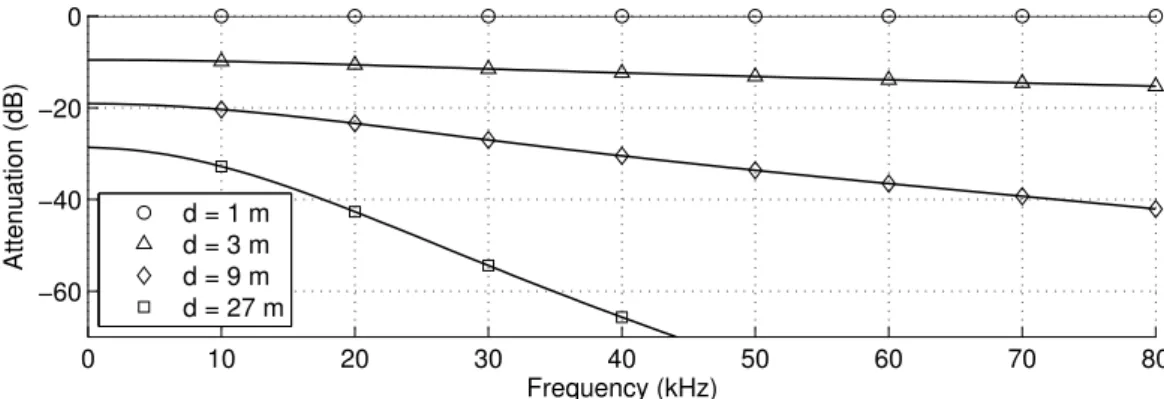
3.10 Wave attenuation variation over frequency for different distances at typical room con-ditions. . . 28
3.11 Impact of the room ambient conditions and the wave frequency into the absorption coefficient in air. . . 30
3.12 Comparison between atmospheric and dispersion attenuation in air. . . 31
3.13 Total attenuation in air for a receiver at 4 m in reference to 1 m. . . 32
3.14 Impulse response with 64 samples length that represents the total air attenuation and the error obtained by the truncation process. . . 32
3.15 Algorithm for reduction of the error in a specific band. . . 33
3.16 Impulse response with 64 samples that represents the total air attenuation and the error obtained by the truncation process using the proposed algorithm. . . 33
3.17 The division of hm(n) in four main IRs. . . 34
3.18 Possible divisions in two quadrilaterals of a complex shape. . . 35
3.19 Example of a room modeled with 10 quadrilaterals. . . 35
3.21 Ultrasonic wave reflection in a wall from a punctual source. . . 36
3.22 Ultrasonic wave reflection in an object. . . 37
3.23 Ray tracing method. . . 38
3.24 Example of ray tracing method using 16 pyramids. . . 39
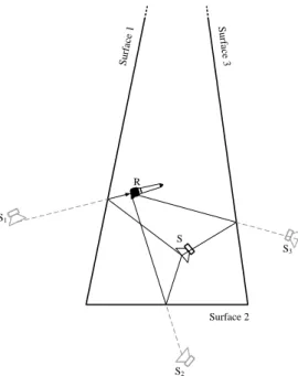
3.25 Virtual Source Method principle. . . 40
3.26 Example of Virtual Sources that produce reflections of first order. . . 41
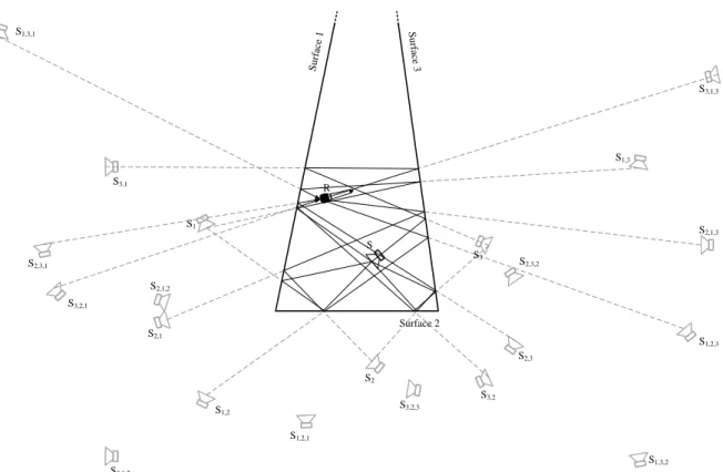
3.27 Example of Virtual Sources that produce reflections of second order. . . 42
3.28 Example of Virtual Sources that produce reflections of third order. . . 42
3.29 Modules and methods interaction in the implemented simulator. . . 43
3.30 Impulse response given by the transfer function module for different azimuths. . . . 44
3.31 Output example of the display room method using the room representation file. . . . 46
3.32 Impulse response given by the propagation process module at 10 m from the source. . 47
3.33 Example of the absolute value of an impulse response given by the get impulse re-sponsemethod considering a maximum of 5 reflections. . . 48
3.34 Simulation time as a function of the number of room surfaces and the maximum number of successive reflections to consider. . . 49
3.35 Simulation time in function of the maximum number of successive reflections to con-sider for different number of sources in the room. . . 50
3.36 Doppler effect produced by the receiver movement. . . 50
3.37 Block diagram for Doppler effect processing. . . 51
3.38 Simulation environment to test the Doppler effect for a receiver with uniform and rectilinear movement. . . 51
3.39 Ultrasonic speaker model used in the simulator. . . 51
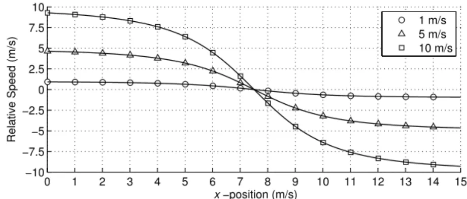
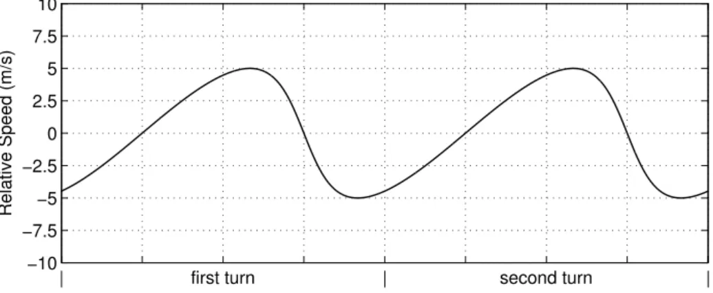
3.40 Relative speed between receiver and source for a receiver with uniform and rectilinear movement. . . 52
3.41 Doppler frequency shift experienced in receiver with uniform and rectilinear movement. 52 3.42 SPL produced by the source as a function of the frequency in the receiver direction. . 53
3.43 Doppler effect in a sinusoidal signal for a receiver with uniform and rectilinear move-ment for three different speeds. . . 54
3.44 Doppler effect in a signal composed by 5 sinusoidal signals for a receiver with uni-form and rectilinear movement for three different speeds. . . 55
3.45 Doppler effect in a BPSK modulated signal for a receiver with uniform and rectilinear movement for three different speeds. . . 56
3.46 Simulation environment to test the Doppler effect for a receiver with uniform and circular movement. . . 57
3.47 Relative speed between the receiver and source for a receiver with uniform and circu-lar movement. . . 57
3.48 Doppler effect and reflection impact into three different signals for a receiver with uniform and circular movement. . . 59
List of Figures
4.2 OFDM example 1. . . 62
4.3 OFDM example 2. . . 63
4.4 Block diagram of the frame prototype. . . 63
4.5 Example of one possible frame. . . 65
4.6 Matched Filter. . . 66
4.7 Pulse detection with DFT. . . 67
4.8 Detection decision block. . . 68
4.9 Probability of false alarm for 500 and 1000 carriers and a threshold value of 100 and 200. . . 71
4.10 Matched filter output for a SNR of 0 dB. . . 72
4.11 Matched filter output for a SNR of -20 dB. . . 72
4.12 Probability of detecting and not detecting the pulse for a signal to noise ratio of 0 dB. 73 4.13 Probability of detect and not detect the pulse for a signal to noise ratio of -20 dB. . . 73
4.14 Probability of detection for the last pulse sample for three different signal to noise ratios. . . 74
4.15 Distance to the source that has a probability of detection greater than 0.99 for different signal to noise ratios. . . 74
4.16 Comparison between an ideal auto-correlation function and the auto-correlation func-tion produced by two pulses with 50 carriers. . . 75
4.17 Representation of the Main-to-Side lobe Ratio. . . 75
4.18 Comparison between the auto-correlation function of two pulses with 50 carriers. . . 76
4.19 Probability of detection for two pulses with different MSR values. . . 76
4.20 MSR minimum, mean and maximum value of an OFDM pulse as a function of the number of carriers. . . 77
4.21 Normalized auto-correlation function expected value for a fixed OFDM pulse size and different number of carriers. . . 77
4.22 Pulse detection with a window at the receiver side. . . 78
4.23 Absolute value of the carriers and an Hamming windows for a OFDM pulse. . . 78
4.24 The normalized auto-correlation function with and without using a Hamming windows. 79 4.25 Example of an OFDM 5000 samples pulse with 1000 carriers with amplitude 1 and random phase. . . 79
4.26 Envelope instantaneous power and real signal instantaneous power for a pulse with narrow-bandwidth. . . 80
4.27 Envelope instantaneous power and real signal instantaneous power for a pulse with high-bandwidth. . . 81
4.28 Impact of high-bandwidth into the PAPR and PMEPR difference. . . 81
4.29 PMEPR value for Newman and Narahashi-Nojima methods as a function of the num-ber of carriers. . . 82
4.30 The iterative algorithm to decrease the PAPR. . . 82
4.31 Algorithm results after 1 million iterations for an 10000 samples OFDM pulse with 100 carriers. . . 83
4.32 Algorithm results after 1 million iterations for an 10000 samples OFDM pulse with 1000 carriers. . . 84 4.33 Chirp pulse example with 1000 samples. . . 85 4.34 Comparison between the spectrum of the OFDM and the Chirp pulse. . . 85 4.35 The OFDM and the Chirp pulse auto-correlation functions. . . 85 4.36 Probability of detection for an OFDM and a Chirp pulse as a function of the Signal to
Noise Ratio. . . 86 4.37 Instantaneous Power Distribution for an OFDM and a Chirp pulse with the same
characteristics. . . 86 4.38 The block diagram of the asynchronous OFDM receiver. . . 87 4.39 Exemplification of a possible pulse detection. . . 88 4.40 Noise performance for BPSK and DBPSK modulation. . . 89 4.41 Block diagram of the frame prototype with a Chirp and DBPSK. . . 89 4.42 Pulse duration values for a 10000 samples OFDM pulse with 1000 carriers sampling
at 250 kHz. . . 89 4.43 Comparison between the bit error rate of the OFDM and the Chirp + DBPSK pulse
in the presence of white Gaussian noise. . . 90 4.44 Comparison between the bit error rate of the OFDM and the Chirp + DBPSK pulse
for a SNR of 0 dB in the presence of synchronization jitter. . . 91 4.45 System representation used to compare the pulse performance in the presence of a
single reflection. . . 91 4.46 Impulse response used to compare the pulse performance in the presence of a single
reflection with the same amplitude. Where ϕ is uniformly distributed between 0 and 2π. 91 4.47 Bit error rate for OFDM and Chirp + DBPSK in the presence of a single reflection
with the same amplitude for a 10 dB SNR. . . 92 4.48 Impulse response used to compare the pulse performance in the presence of a single
reflection where its amplitude decreases with the arrival time difference. . . 92 4.49 Bit error rate for OFDM and Chirp + DBPSK in the presence of a single reflection
where its amplitude decreases with the arrival time difference. . . 93 4.50 Impulse response used to compare the pulse performance in the presence of multiple
reflections where the amplitude decreases with the arrival time difference. . . 93 4.51 Example of an impulse response used to compare the pulse performance of the two
methods in the presence of multiple reflections. . . 94 4.52 Bit error rate for OFDM and Chirp + DBPSK in the presence of multiple reflections
where there amplitude decreases with the arrival time difference. . . 94 4.53 Bit error rate for OFDM and Chirp + DBPSK in the presence of multiple reflections
for an impulse response duration of 100 samples. . . 95 4.54 Bit error rate for OFDM and Chirp + DBPSK in the presence of multiple reflections
for an impulse response duration of 500 samples. . . 95 4.55 Bit error rate for OFDM and Chirp + DBPSK in the presence of multiple reflections
List of Figures
4.56 Room shape implemented into the simulator to compare the pulse performances in the presence of multipath. . . 96 4.57 Ultrasonic speaker model used in the simulator. . . 96 4.58 Ultrasonic receiver positions to compare the pulse performance in the presence of
multipath. . . 97 4.59 Bit error rate for each x position for 100 bits and a bandwidth of 2.5 kHz. . . 97 4.60 Bit error rate for each x position for 1000 bits and a bandwidth of 25 kHz. . . 98 5.1 Example of the proposed ultrasonic location system architecture. . . 100 5.2 Different types of nodes present in the proposed architecture. . . 100 5.3 Beacon location process example. . . 101 5.4 Mobile location process example. . . 102 5.5 Beacons clock model and the ideal clock. . . 103 5.6 The three ways that the time messages can be exchanged between beacons for clock
synchronization. . . 104 5.7 Time messages exchanged in the synchronization process between two beacons for
the two-way message exchange. . . 105 5.8 Time messages exchanged in the synchronization process between two beacons for
the one-way message dissemination. . . 106 5.9 Connectivity between beacons in the level discovery phase. . . 108 5.10 Messages exchanged between two beacons in the synchronization phase. . . 109 5.11 Messages exchanged between two beacons in the synchronization phase for the
mod-ified TPSN. . . 111 5.12 Example of a messages exchanged between beacons in the synchronization phase.
The solid line represents frequent connectivity and the dashed lines sporadic connec-tivity. . . 111 5.13 Example of the three messages exchanged for beacon 2 synchronization. . . 112 5.14 Network beacons in a hexagonal shape cells for clock synchronization in a room with
18 m × 66.5 m. . . 113 5.15 Hierarchy level of each beacon in the networks for beacon 1 as reference beacon. . . 114 5.16 Clock results after the synchronization process for each odd level in the hierarchy for
ideal synchronization process. . . 115 5.17 Hierarchy level of each beacon in the networks for beacon 48 as reference beacon. . . 116 5.18 Clock offset error relative to the master clock as a function of the synchronization
processes for four different levels in the hierarchy, considering a time of arrival error standard deviation of 1 ms. . . 116 5.19 Standard deviation of the clock error in each level in the hierarchy for a million of
synchronization processes, considering a time of arrival error with a standard devia-tion of 1 ms. . . 117 5.20 Distance measurements obtained in each beacon divided in three different classes.
5.21 Distance measurements obtained in each beacon divided in three different classes. Considering beacon 48 as the reference node. . . 120 5.22 Network beacons in a hexagonal shape cells for clock synchronization in a room with
18 m × 66.5 m for a maximum range of 10 m. . . 121 5.23 Hierarchy level of each beacon in the networks for beacon 1 as reference beacon and
considering a maximum range of 10 m. . . 121 5.24 Hierarchy level of each beacon in the networks for beacon 48 as reference beacon and
considering a maximum range of 10 m. . . 122 5.25 Total number of distance measurements obtained in each beacon. Considering beacon
1 as the reference node and a maximum range of 10 m. . . 122 5.26 Total number of distance measurements obtained in each beacon. Considering beacon
48 as the reference node and a maximum range of 10 m. . . 122 5.27 Example of a simple node displacement with several different variables. . . 124 5.28 Example of the location message broadcast from 4 beacons. . . 125 5.29 Location messages received by the mobile at different times from 4 beacons. . . 125 5.30 All the distance measures obtained by beacon 4 during the time synchronization process.128 5.31 Beacons location algorithm running in each beacon. . . 132 5.32 Simulation environment to test the mobile location algorithm. . . 133 5.33 Average error for x and z coordinate, considering a distance measurement error with
1 cm of standard deviation. . . 134 5.34 Average error for x and z coordinate, considering a beacon position error with 1 cm
of standard deviation. . . 135 5.35 Average error for x and z coordinate, considering a beacon position and distance error
with 1 cm of standard deviation. . . 136 5.36 Average error for each coordinate, considering beacon position (a) or distance error
(b) as a function of noise standard deviation. . . 137 5.37 Four different anchor beacons arrangement with different number of anchor beacons. 138 5.38 Average position error for each coordinate in the four anchor distributions after one
thousand synchronization processes. . . 140 5.39 The error of beacon’s x-coordinate, in millimeter, for the four anchor beacons
distri-bution after one thousand synchronization processes. . . 141 5.40 The error of beacon’s z-coordinate, in millimeter, for the four anchor beacons
distri-bution after one thousand synchronization processes. . . 142 5.41 Error of the x-coordinate after 250 synchronization processes for three different
num-bers of iterations between synchronization processes. . . 143 5.42 Comparison between the original dw-MDS and the proposed modified dw-MDS
al-gorithm. . . 144 5.43 Average position error for each coordinate as a function of the synchronization
pro-cesses. . . 145 5.44 Impact in coordinates errors after the replacement of the failure beacon 33. . . 146
List of Figures
6.1 Measurement system used for practical tests. . . 147 6.2 Data acquisition hardware. . . 148 6.3 Br¨uel & Kjær 4954-A microphone, its power supply and its frequency response. . . . 148 6.4 Microphone amplifier and its frequency response. . . 149 6.5 Speaker buffer and speaker Kemo L10 and its frequency response. . . 149 6.6 Scheme of the sound speed measurement experiments. . . 150 6.7 Amplitude histogram of the OFDM pulse samples used for sound speed measurement. 150 6.8 Speaker and microphone 5 m apart. . . 151 6.9 Signal obtained at the matched filter output and the threshold value used to measure
the sound speed at 5 m. . . 151 6.10 Time-of-flight measurements and mean value. . . 151 6.11 Temperature presented in the thermometer during the first experiment. . . 152 6.12 The temperature obtained from the TOF measurements and the temperature presented
in the thermometer during the second experiment. . . 152 6.13 Sports pavilion used to measure the air attenuation due to absorption. . . 152 6.14 Scheme used to measure the air attenuation due to absorption. . . 153 6.15 Comparison between the measured atmospheric absorption and the expected
theoret-ical value. . . 153 6.16 Atmospheric attenuation due absorption that results from the frequency response
comparison for 46 different distances speaker-microphone. . . 154 6.17 Scheme used to test the simulator for one reflection. . . 154 6.18 Simulation environment used to test the simulator for a single reflection case. . . 155 6.19 Impulse response comparison for a single reflection. . . 155 6.20 Simulation environment used to test the simulator in a complex room. . . 157 6.21 Measurement points in the test of a complex room. . . 157 6.22 Impulse response comparison for a complex room shape. . . 158 6.23 Simulation environment for simulators comparison. . . 159 6.24 Comparison between the impulse response of the modified Lehmann’s simulator and
that of the proposed simulator. . . 161 6.25 Delay error for propagation delay of 2 m (around 1747.5 samples). . . 162 6.26 Shadowing effect produced by the slow decay of a strong impulse. . . 162 6.27 Empirical probability density function for the real and imaginary part and the true
probability density function for a normal distribution with the same variance. . . 163 6.28 Scheme used to evaluate the probability of detection. . . 164 6.29 Probability of detection estimation using a real setup and the simulator for the last
pulse sample considering a probability of false alarm of 10−6. . . 164 6.30 Scheme for testing the accuracy and repeatability of the distance measurement process. 165 6.31 Box-and-whisker diagram of the absolute error for 25 trials in the distance
measure-ment of 5 m. The central mark is the median, the edges of the box are the 25th and 75th percentiles, the whiskers extend to the most extreme data points. . . 165 6.32 Absolute error in the distance measurement between 1 m and 5.5 m. . . 166
6.33 Box-and-whisker diagram of the absolute error of 46 equally spaced positions be-tween 1 m and 5.5 m from the speaker. . . 166 6.34 Box-and-whisker diagram of the absolute error of 46 equally spaced positions
be-tween 1 m and 5.5 m from the speaker using interpolation in the distance estimation. 166 6.35 Simulation environment to test the location system. . . 167 6.36 Hierarchy level of each beacon in the network considering beacon 1 as reference
beacon and a maximum communication range of 5 m. . . 167 6.37 Time-line for the initial stage. . . 168 6.38 Time-line for the established stage. . . 168 6.39 The average beacon’s position error. . . 169 6.40 The average beacon’s position error during 9 days long. . . 169 6.41 The average beacon’s position error for each beacon during 9 days long. . . 170 6.42 Number of beacons that a mobile could receive information from at 1.5 m from the
floor, considering a 5 m range. . . 171 6.43 Average error for x and z coordinates during 9 days after the initial stage. . . 172 6.44 Average error for x and z coordinates during 9 days after the initial stage considering
a maximum range of 5 m. . . 173 A.1 Microphone amplifier propose. . . A-1 A.2 Implemented microphone amplifier. . . A-2 A.3 Measuring tool used to evaluate the frequency response of the microphone amplifier. A-2 A.4 Microphone amplifier frequency response for each gain position. . . A-4 A.5 Microphone Amplifier Schematic – Audio Amplifier. . . A-5 A.6 Microphone Amplifier Schematic – Power Supply. . . A-5 A.7 Microphone Amplifier Board Layout – Top Layer. . . A-6 A.8 Microphone Amplifier Board Layout – Bottom Layer. . . A-6 B.1 The time delay of a continuous signal. . . B-1 B.2 The time delay of a discrete signal. . . B-2 B.3 Ideal delay filter. . . B-2 B.4 Example of an impulse response for an integer and a non integer delay. . . B-3 B.5 Example of two impulse responses for Lagrange fractional delay filter with 16.1 and
16.5 samples delay and order 32. . . B-4 B.6 Frequency Response and Group Delay for the examples of Figure B.5. . . B-4 B.7 Frequency Response and Group Delay for a Lagrange fractional delay filter with delay
of 0.5 samples and order 32. . . B-4 B.8 Maximum frequency response gain for different delays, considering a 32 order filter. B-5 B.9 Frequency Response and Group Delay of 15th order Lagrange fractional delay filters
for different delays. . . B-6 B.10 Frequency Response and Group Delay of 16th order Lagrange fractional delay filters
List of Figures
B.11 Frequency Response and Group Delay of 31st order Lagrange fractional delay filters for different delays. . . B-7 B.12 Frequency Response and Group Delay of 32nd order Lagrange fractional delay filters
for different delays. . . B-7 B.13 Fractional delay impact into the group delay and frequency response errors for a 32nd
order filter. . . B-8 B.14 Filter order impact into the group delay and frequency response errors. The presented
error is the maximum error for a fractional delay between 0 and 1. . . B-8 B.15 Fractional delay filter bandwidth as a function of the filter order and the fractional delay.B-8
L
IST OF
T
ABLES
2.1 Comparison of some indoor location systems. . . 19 3.1 Characteristics of the computer and software used in the simulator performance tests. 48 5.1 The results of the message broadcasting after each beacon synchronization. . . 112 5.2 The collected distances between beacons in each beacon after all beacons
synchro-nization. . . 113 6.1 Main differences between the proposed simulator and the modified Lehmann’s
simu-lator. . . 160 6.2 Lilliefors test result for the 300000 frequency samples, using significance level of 5%. 163 A.1 Main characteristics of THAT 1510 and INA110, components used in the microphone
amplifier. . . A-1 A.2 All possible gains provided by the microphone amplifier. . . A-2 A.3 Microphone amplifier gain for each gain position and frequency. . . A-3
A
CRONYMS
1D one dimensional. 16
2D two dimensional. 11, 14–16, 38, 99, 127, 130 3D three dimensional. 11–13, 17, 35, 58, 127, 130 ACF auto-correlation function. 75, 77, 78, 85 AOA angle of arrival. 10, 11, 14
BER bit error rate. 61, 88–94, 96, 176
BPSK binary phase shift keying. 13, 53, 58, 62, 63, 88 CDMA code division multiple access. 12, 13
DBPSK differential binary phase shift keying. 3, 4, 88–92, 94, 96, 176 DFT discrete Fourier transform. 33, 66, 67, 162
DSSS direct-sequence spread spectrum. 12
dw-MDS distributed weighted-multidimensional scaling. 128, 130, 144, 177 FDMA frequency division multiple access. 125
FFT fast Fourier transform. 61, 90, 91
FHSS frequency hopping spread spectrum. 13 FIR finite impulse response. 66
FT Fourier transform. 69, 153
GNSS global navigation satellite systems. 2 GPS global positioning system. 2, 7, 108
GSM global system for mobile communications. 7 ID identification. 10, 11, 14, 110, 111, 171
IDFT inverse discrete Fourier transform. 33, 66, 67 IFFT inverse fast Fourier transform. 61, 62
IFT inverse Fourier transform. 31, 161 IR impulse response. 21–24, 26, 31–34, 37, 38, 44, 47, 50, 53, 91–94, 153, 154, 157, 176 ISI inter-symbolic-interference. 61, 63, 65, 91, 92, 94, 96 LOS line-of-sight. 157 LS location system. 1–3, 7–16, 18 MDF medium-density fiberboard. 156 MDS multidimensional scaling. 127, 128 MEMS micro electro-mechanical systems. 14
MF matched filter. 66–68, 72, 75, 78, 85, 87, 151, 163, 165 MSR main-to-side lobe ratio. 75–77, 85
NLOS non-line-of-sight. 123, 157
OFDM orthogonal frequency division multiplexing. 3, 4, 61–63, 66–68, 75–79, 81–83, 85–92, 94, 96, 150, 151, 153, 164, 165, 176, 178
PAPR peak-to-average power ratio. 79–83, 86, 150, 176, 178 PC personal computer. 10, 11, 17, 48, 147
PL powerline. 14
PLP powerline positioning. 14
PMEPR peak-to-mean envelope power ratio. 80–83, 86 PSK phase shift keying. 61, 88
QAM quadrature amplitude modulation. 61, 88
RF radio frequency. 2–4, 9, 11–14, 17, 18, 21, 24, 105, 175–177 RFID radio frequency Identification. 14–16
SNR signal to noise ratio. 66, 69, 70, 72–74, 77, 78, 85, 90–93, 163 SPL sound pressure level. 53
Acronyms
TDOA time difference of arrival. 3, 4, 17, 99, 126, 177 TOA time of arrival. 11, 126, 134
TOF time of flight. 3, 4, 9, 11, 12, 14, 17, 18, 61, 62, 65, 75, 76, 78, 87, 116, 124, 150, 152, 164, 176, 178
TPSN timing-sync protocol for sensor networks. 4, 107, 110–112, 177 UDP user datagram protocol. 15
US ultrasounds. 9–14, 17, 18, 21, 24, 58, 61, 63, 65, 80, 87, 94, 96, 100, 101, 105, 113, 121, 123 UWB ultrawideband. 2
WiFi wireless fidelity. 15
WLAN wireless local area network. 14–16 WSN wireless sensor network. 104, 105, 107
L
IST OF
S
YMBOLS
α absorption coefficient in air. 28–31, 64, 65 P acoustic air pressure. 25, 27–31
T air temperature. 25, 26, 28, 30 AT atmospheric attenuation. 31 χ2
2 chi-squared distribution with 2 degrees of freedom. 69, 70, 72 nτ delay in samples due to the wave time of flight. 65
δi, j distance measurement between the node i and j. 124 d distance between two nodes. 106, 109, 124
fD Doppler frequency shift. 52, 58
di, j euclidean distance between the position i and j. 124 ζ local clock for each node. 103, 104
φ local clock offset. 103, 104, 106, 107, 109, 126 fmax maximum frequency of the signal. 64
C node coordinates. 111, 124, 125 L number of beacons. 126
Nc number of carriers. 64, 67–71, 73, 76, 77, 89, 90
Pd probability of detection. 70–73, 75, 85 Pf a probability of false alarm. 70–73, 75, 85
τ propagation delay due to the wave time of flight. 106, 109, 126 Tp pulse duration. 64
N pulse size. 67, 70, 73, 75, 77, 89, 90
vr relative speed between the source and the receiver. 52, 64 fs sampling frequency. 32, 65, 90 σ2 signal variance. 65, 69–71 B system bandwidth. 64, 90 γ threshold. 68, 70–72, 75, 90 ς time stamp. 105–107, 109, 111, 117, 125, 126
CHAPTER1
I
NTRODUCTION
The need for location has been a companion of animals and humans during their evolution path. It has been used to get food and migrate to find better life conditions. For example, geese could travel several hundreds of kilometers keeping their relative position constant in the formation. Moreover, they could return to their initial position after traveling some thousands of kilometers without getting lost, see Figure 1.1a [1]. More recently, location techniques and systems, based on the Sun and stars, were used to conquer the seas and traveling far distances in open seas without getting lost. To accomplish that, several complex instruments were invented, Figure 1.1b presents an example. These instruments were used with two main goals: to display how the sky was or will be at a specific position or to obtain the latitude for the current position. The latitude could be easily obtain by observing the only available references, the sun during the daylight and the stars at night. Therefore, they were very used mainly by the Portuguese and the Castilians during the beginning of discoveries. Nevertheless,
(a) Geese travel around 2700 Km in their migration. After the initial mess the geese rapidly get their known V formation (see the circle in the picture). Source: [1].
(b) Astrolabe (left) used to locate and predict the po-sition of celestial objects, and Mariner’s Astrolabe (right) used to obtain the latitude of a ship at sea. Source: [2].
Figure 1.1: Location is a valuable tool for animals and for humans.
they had a huge problem, it was impossible to obtain longitude. Therefore to reach a specific place the ship was sailed to the desired latitude and then it must be sailed along the latitude line, to east or west, until reaching the desired destination. Moreover they could not be used if the sky was not clear. Since then, in order to accommodate the most demanding human needs for location, science has been providing new ways using several technologies for different purposes.
Nowadays, location systems (LSs) are a built-in feature of several complex systems, such as robots. It is present in the automation industry, autonomous navigation, emergency callers, explo-ration of unreachable places on Earth and space, etc... Even at home, where robots start to have a daily presence, we have autonomous mowers able to cut the grass, vacuum cleaners that can clean the floor without human intervention and so many other examples. To exemplify the present day technol-ogy diversity, Figure 1.2 presents the technoltechnol-ogy currently used in several LSs for indoor and outdoor applications and their accuracy and maturity. The maturity was divided in three categories: Research Labs, Custom Systems and Consumer Systems. The Research Labs represents all systems that are still
in the research laboratories and so not available to public. The Custom Systems represents all system that are available but their use is restrict or very specific to an application. Finally, the Consumer Systemsrepresents all the systems that are easily available and could be found in several everyday objects. For outdoor location, the location systems are dominated by the global navigation satellite
1 mm 1 cm 10 cm 1 m 10 m Indoor Outdoor ≥100 m RF Based Light Based Sound Based
Figure 1.2: The accuracy and maturity of several technologies currently used for indoor and outdoor location. Information collected from [3, 4, 5].
systems (GNSS) (where global positioning system (GPS) is the most known and used). The GNSS are based in the same principle of the ancient location systems, measuring the distance to artificial celestial objects. Nevertheless, there are several solutions based on cellular network infrastructure or wireless networks profiling that could improve the resultant position estimation [4]. In addition to those technologies (see Figure 1.2) there are also some custom systems that could be used to pro-vide an accurate location (ultrawideband (UWB)) or a long battery life (Sunlight). However, those technologies are not provided in our everyday objects and their applicability is very specific.
As it can be seen in Figure 1.2 the outdoor location systems are already in a mature stage, however the same cannot be said for indoor location systems, where the mature system are not able to provide accurate indoor location information due to fading and multipath effects of the buildings on the radio frequency (RF) signal [6].
As a result of the increasing necessity to provide an indoor location system that is adequate to locate people, objects (e.g., robots) inside a building (e.g., factory, hospital, school, home, etc.) it is important to provide a LS that is able to provide a position with an accuracy in the centimeter order. Regarding the technology chart present in Figure 1.2 the best suited technology is the ultrasounds. Although, the ultrasonic based custom systems and the majority of the system in laboratory use an auxiliary RF-channel to perform location or the user needs to provide a set of a priori information.
1.1 Objectives
The main goal of this thesis is the development of an indoor location system using only ultrasonic signals, resulting in a RF-free location system. The proposed LS is manly designed to be implemented in indoor environments, nevertheless, it suits any environment where the use of RF is not allowed or it is strongly mitigated and the ultrasonic propagation is favorable. One of the best examples of this environments is underwater. In such environment the RF waves are strongly attenuated due to the water conductivity, especially in the seawater case [7]. Additionally, the ultrasonic propagation in water is more favorable than in air, ultrasonic signals travel 4 times faster in water than in air.
In the proposed LS, the ultrasonic signals will be used to get distance information, from time of flight (TOF), and also to implement data communication. For data communication and TOF measure-ment, an ultrasonic pulse that uses orthogonal frequency division multiplexing (OFDM) and differen-tial binary phase shift keying (DBPSK) is proposed. This proposed pulse was designed to be robust to the acoustic indoor environment demands.
The proposed location system uses a support network of fixed beacons, attached to the ceiling or walls of a room, and mobiles that need location information inside that particular room. In the network of beacons there are some special beacons, called anchor beacons. The anchor beacons have a predetermined position and they are the reference for all the network to compute the other beacons position. Each beacon is completely autonomous and as a result of this a clock synchronization protocol was proposed, this protocol will allow, not only, beacons to synchronize their clocks but also to obtain the distance measurements between them by exchanging only three messages from time to time. The beacons coordinates are obtained by the minimization of a local cost function using an iterative algorithm allowing to take advantage not only from the distance measurements to its neighbors but also from the distance measurements between the neighbors. This approach reduces human intervention during the network implementation and failure beacons can be easily replaced without compromising the network operation. Mobiles are responsible to locate themselves applying a very simple algorithm based on the time difference of arrival (TDOA). This algorithm uses the ultrasonic messages received from the nearby beacons with the message time-stamp and the beacon’s coordinates. This approach allows the location system to be independent of the number of mobiles and will provide a high degree of privacy since the mobiles do not need to transmit any message.
In addition to this, a simplified model of the acoustical channel was developed resulting in an ul-trasonic simulator for indoor environments. This simulator proved to be very accurate and a valuable tool to simulate the location system behavior under controlled conditions.
1.1
Objectives
The Ph.D. thesis work has been concentrated into achieve the following, initially proposed, ob-jectives:
• A simplified simulator for ultrasound acoustical propagation in indoor environments;
• A technique to perform TOF measurements and data transmission over the shared ultrasonic acoustic channel;
• A method to perform location using ultrasonic signals and avoiding the use of an auxiliary radio frequency channel;
• A distributed algorithm to perform a mobile location using the TOF measurements from the network of beacons.
1.2
Contributions
This Ph.D. work presents several contributions that will be detailed. The first contribution is an ultrasonic room simulator that is able to deal with high bandwidth ultrasonic signals. This simulator is capable of handling the multiple reflections present in a room which could be produced by the room walls or by the objects inside it. Moreover, it takes into account the beam patterns of the used transducers as well as the ultrasonic wave propagation losses. Additionally the simulator may be used to simulate the Doppler effect for any movement. In the end, the proposed simulator proved to be a valuable tool to study and compare different location algorithms and acoustic pulses under controlled conditions.
Another, extremely relevant contribution is the ultrasonic pulse design that allows TOF measure-ment simultaneously with ultrasonic communication. This ultrasonic pulse is robust to environmeasure-ments with strong multipath when used to measure the TOF and to transmit data. This pulse makes use of OFDM and DBPSK. Additionally, some techniques are suggested, to reach, and sometimes surpass, the most frequently used TOF measurement pulse, the chirp pulse.
By combining this first two contributions the author designed a RF-free ultrasonic location sys-tem with a reduced setup time and low maintenance cost, where failure nodes can be easily replaced without the need of a qualified technician. To accomplish that, the proposed location system uses a synchronous network of beacons where a proposed location algorithm will allow each beacon to com-pute its location using TOF measurements from its neighbors. The beacon location is performed using a modified version of the distributed weighted-multidimensional scaling proposed in [8]. Which is a distributed location algorithm that can deal with a variable number of neighbors and it can improve the accuracy of the location by minimizing a local cost function. Each beacon on the network period-ically transmits an ultrasonic message. Thereafter, the mobiles, by collecting a set of this messages, can compute their location using common TDOA algorithm.
The last important contribution is related with the process of synchronizing the beacon’s network and obtaining the information of distance between the beacons. The proposed synchronization tech-nique was based in the timing-sync protocol for sensor networks (TPSN) proposed by Saurabh Ganer-iwal, et. al, in [9]. This synchronization technique was modified using a three messages exchange mechanism which allows to take advantage of the neighbors synchronization processes. Therefore, by using the proposed approach the distance measurement process is embedded in the network syn-chronization process. As a result of this, each beacon will obtain the distance information of its neighborhood without exchanging any additional message.
1.3 Organization
1.3
Organization
This thesis is organized in seven chapters. Chapter 2 presents a brief introduction to indoor loca-tion systems and the related work on this field, as well as the state-of-art of indoor localoca-tions systems with a special emphasis on ultrasonic indoor location systems. An ultrasonic simulator for indoor environments is presented in Chapter 3. Chapter 4 focuses on the ultrasonic pulse that will allow data communication and distance measurement, comparing it to some commonly used techniques. Chapter 5 presents the proposed location system architecture with all the details about beacons lo-cation, clock synchronization and mobile lolo-cation, as well as an exhaustive discussion with some examples of its performance and failure tolerance. Chapter 6 looks at the overall results, validating the used models by field tests and presents a final example combining all the algorithms proposed for the location system in Chapter 5. Finally, in Chapter 7 the Ph.D. work will be summarized and some proposals for future research directions will be introduced in order to improve the proposed location system.
CHAPTER2
I
NDOOR
L
OCATION
S
YSTEMS
The GPS is the most popular system for outdoor location achieving an accuracy between 20 to 30 m [10]. Recently, there has been great interest in using the antennas infrastructure of the global system for mobile communications (GSM) to perform outdoor location without the need of any additional hardware besides the mobile phones. The expected accuracy of such systems in urban areas is about 100 m [11, 12]. However, this accuracy is not enough for indoor applications. This chapter presents an introduction to indoor location and some notation that it will be used during the following chapters. This chapter, starts by presenting the indoor location system characterization in Section 2.1. After that, in Section 2.2 the three main technologies used in indoor location system are presented. Which will be detailed in the follow four sections: 2.3, 2.4, 2.5, and 2.6, and compared in Section 2.7. At the end of this chapter the typical approach followed by the ultrasonic location system state-of-art will be presented.
2.1
Location System Characterization
2.1.1 Levels of Location
An indoor LS can be characterized by its level of location which results from the LS accuracy and characteristics. Therefore, an indoor LS can be dived into three main location levels:
Building At building level the LS only needs to provide the information in which part of building the object is (e.g., first floor, north side; entrance; etc.). For that propose the accuracy needs to be around 10 m.
Room At room level the LS needs to provide the exact room of a building where the object is (e.g., bathroom, kitchen, master bedroom, etc). In a such system the accuracy needs to be around 1 m.
Exact At exact level the LS provides the exact position of the object inside a room in reference to the room or the building, normally it is presented as Cartesian coordinates (e.g. (4, 2); (3, 5, 1)). Resulting into an accuracy need of around 10 cm or less.
Figure 2.1 presents a comparison between this three levels of accuracy in a building floor. At the building level the LS gives the information that the object is in the first floor of that particular building. At the room level the LS, apart from the floor, could also specify that the object is in Room 2 of the first floor. In contrast, the exact level provides the exact position in the Room 2 where the object is (7, 9) in this example.
Room 4 Room 3 Room 1 Room 2 Room 3 Room 4 1st Floor Building level 2 4 6 8 10 12 2 4 6 8 10 12 Room 1 Room 2 Room 3 Room 4 1st Floor Room level 2 4 6 8 10 12 2 4 6 8 10 12 1 st Floor Exact level 2 4 6 8 10 12 2 4 6 8 10 12 y y y x x x Room 1 Room 2
Figure 2.1: Comparison between the three levels of location.
2.1.2 Network Topology and Operation Mode
The indoor LS solutions can be classified by the network topology used and the operation mode. In the network topology the system is characterized by the use of an auxiliary network of reference nodes (designated by beacons). The network of beacons is normally utilized to assure complete field coverage where the location system must operate. Typically, in a LS with a network of beacons the nodes connect only with the beacons and they do not connect to other nodes. However, the system can operate without this network of beacons, this is typically used for mutual location (e.g. robot formation), in this topology the nodes connect to each others in order to perform the location. Figure 2.2 shows the difference between LS with an auxiliary network of beacons and without it.
Network with fixed beacons Network with mutual location
Beacon Mobile Node
Figure 2.2: The use of an auxiliary network of beacons.
The operation mode can be classified according to where the location algorithm is performed. In the centralized mode the location algorithm is computed in a central node, designed specifi-cally for that propose, the nodes connect to this central node and send to it the relevant information to perform the nodes location, the central node computes all the nodes location and could share the location information with the remaining nodes. The option to share or not the location information depends on the LS purpose and security or privacy policies. In this type of systems the connectivity with the central node is mandatory, restricting the network range or increasing the communication complexity.
2.2 Technologies for Indoor Environments
based on the information exchanged with its neighbors. This approach typically reduces the connec-tivity problem to the central node. However, it is more demanding in respect to the nodes processing capabilities.
Figure 2.3 presents the difference between centralized and distributed location algorithms.
Centralized operation mode Distributed operation mode
Node
Loc. algorithm
Figure 2.3: The use of a central node running the location algorithm.
2.2
Technologies for Indoor Environments
To achieve the levels of accuracy required in indoor environments, there are three major types of technologies that could be used [4]:
• Infrared based;
• Ultrasounds (US) based; • RF based.
LS based on infrared radiation usually provides a room level location, they use a network of beacons that receive an infrared unique identifier from a source placed on the object, the system typically operates in the centralized mode. On the other hand, the majority of the LS based on US, provide the exact location of the node and they normally perform the node location by measuring the distance (using TOF) between nodes (in mutual location) and other reference points (with a network of bea-cons). Moreover, these systems can operate either in centralized or distributed mode. LS based on RF provides a room level location and sometimes the exact location, for that purposed, they usually use the power of the received signal from a network of beacons and compare it to a set of amplitudes, captured previously in several positions. This information is further used to infer about the node location (they typically operate in the centralized mode).
This three main technologies will be detailed and the state-of-art of each one will be presented in the following sections.
2.3
Location Systems based on Infrareds
This section presents two different location systems based on infrared: the Active Badge [13] and the InfraRed Indoor Scout [14]. The Active Badge is a centralized location system with a network of
sensors that detect the location of an infrared emitter tag. The InfraRed Indoor Scout is a centralized location system that uses a stereo camera to detect the location of an infrared emitter tag.
2.3.1 Active Badge
The Active Badge [13] is one of the first indoor location systems, it was introduced in 1992. The Active Badge was designed to locate a tag inside a building, giving a symbolic position (e.g. the room where the tag is). Each tag sends a unique infrared identification (ID) with approximately 100 ms duration every 15 seconds. Therefore, a wired network of infrared sensors placed in the building receives the infrared signal and sends it to a master station, in the network, which processes all the received data and computes the tag symbolic location. The Active Badge is a very simple indoor location system, which provides room accuracy. The most expensive part of the system is the sensor network and it is a solution with some drawbacks: short infrared range, the need for line-of-sight operation and external light interference (e.g., Sun, light bulb). However, the tag’s battery has a lifetime of one year, which is reasonable for office applications.
2.3.2 InfraRed Indoor Scout
The InfraRed Indoor Scout [14] uses an infrared emitting tag and a stationary mounted stereo camera to locate the objects. The stereo camera is built with two cheap USB cameras (with 120◦ lenses and an infrared filter) placed at 20 cm from each other. The stereo camera receives the infrared signal and the host personal computer (PC) measures its angle of arrival (AOA) at the two cameras, therefore, the tag location is computed by triangulation. The InfraRed Indoor Scout is a very cheap indoor location system that uses off-the-shelf components to compute tag location. Moreover the number of tags does not significantly increases the location processing cost. Furthermore the system can cover a room with 15.1 × 9 m with 16,7 cm of accuracy. Nevertheless, stereo camera calibration is one of the main issues, mainly because the optical cameras are far from ideal.
2.4
Location Systems based on Ultrasounds
This section presents eight different LSs based on US: the Active Bat [15], the Cricket location system [16, 17], the location system from F. Rivard and et al. [18], the Parrot [19], the Dolphin [20], the 3D-LOCUS [21], the M. Hazas and A. Hopper’s system [22] and the J. Gonzalez and C. Bleakley location system [23]. These location systems use two modes of operation: centralized and local. In centralized mode (Active Bat, 3D-LOCUS and Hazas’ LS) the nodes send an unique ultrasonic pulse ID and a network of ultrasonic sensors, with well known locations, receive this pulse and compute the location of each node. In the local mode there are two setup possibilities: using an auxiliary sensor network (Cricket, Hazas’ LS and Gonzalez’s) or using a distributed system (Rivard’s LS, Parrot and Dolphin). In the mode with an auxiliary network of ultrasonic sensors, each sensor in the network with well known location sends an unique ultrasonic pulse ID and the object receives this pulse and computes its location. In the distributed mode each object sends an unique ultrasonic
2.4 Location Systems based on Ultrasounds
pulse ID and its location (if it is known) and the other objects receive these pulses and compute their location.
2.4.1 Active Bat
The Active Bat [15] is a three dimensional (3D) location system that uses US and an auxiliary RF channel to perform the 3D location of a tag (10 × 6 × 2 cm). Every 200 ms a radio message is sent using the auxiliary RF channel (at 418 MHz), this message contains the ID (16 bits) of the tag that the system wants to localize. Therefore, the tag with that ID sends a 50 µs ultrasonic pulse at 40 kHz using an hemispherical array of 5 US transducers. A matrix of ultrasonic receivers, mounted in the ceiling at 120 cm from each other, receives the ultrasonic pulse and sends the times of arrival (TOAs) to a central PC. This central PC computes the tag location by multilateration. Results have shown an accuracy of 8 cm in 98% of the cases; moreover, the PC can locate up to 25 tags in each second. On the other hand, the ceiling ultrasonic receiver matrix increases the infrastructure cost, installation time and reduces the system scalability.
2.4.2 Cricket
The Cricket LS [16, 17] allows a tag to localize itself and get its orientation, providing user privacy, by using an ultrasonic and a RF receiver. The Cricket LS uses several ultrasonic and RF emitters (mounted on the ceiling or on the wall). These emitters provide the signal reference that allows the tag to localize and orientate itself. These emitters randomly send a 47 ms RF signal (at 418 MHz) and a 125 µs ultrasonic pulse (at 40 kHz). The RF signal carries the emitter location (3×2 bytes), its ID (8 bytes) and the room ID (8 bytes). The tags receive the RF signal and the ultrasonic pulse from each emitter and compute the distance to them (using the TOF). The Cricket LS uses cheap hardware, each emitter or receiver costs less than 10$ and provides an accuracy of 10 cm. Moreover, the Cricket Location System has a high level of scalability, although, the system consumes some power (about 15 mW per device).
2.4.3 Rivard’s Location System
The LS from F. Rivard et al. [18] was designed to be used in multi-robot systems and it gives, to each robot, a relative location in two dimensional (2D). Therefore, this LS outputs the distance between robots and the angle between them. For that purpose, the system uses US signals (25.7 kHz) and an auxiliary RF channel (433.92 MHz) to measure the distance (using TOF) and the angle between robots. The system has one ultrasonic transmitter and two receivers (to compute the AOA). Moreover, each robot has a unique ID and it is synchronized with the other robots, to avoid the interference between the sent ultrasonic pulses. Each robot sends an ultrasonic pulse using round robin scheduling with a time watchdog (to keep the system working if some robot fails) and at the same time it signals the other robots using the RF auxiliary channel. The system presents an absolute average error of 8 mm and 3◦with a standard deviations of 8 mm and 3◦ respectively. However the main bottleneck of the system is its power consumption, 1.73 W.
2.4.4 Parrot
The Parrot system [19] is based on a network of tags (Parrots). Each tag uses four ultrasonic transmitters and receivers (40 kHz) and an auxiliary RF channel for synchronization and data com-munication. The system randomly sorts the tags in a queue and the first tag in the queue sends an ultrasonic pulse and RF signal. The other tags receive these signals and compute the distance to that tag using the TOF (time difference between RF and the US pulse). Therefore, this tag goes to the end of the queue and the first tag in the queue behaves the same way of the previous one, and so on. Moreover, the RF link between the tags is used also to communicate the measured distances from one tag to the others. As a result of this, this LS eliminates the necessity of a central system to compute the tags location, so each tag computes its location locally from the information given by the other tags. This location system exhibits an accuracy of 2 cm with a standard deviation of 4 cm and it can work up to 15 m.
2.4.5 Dolphin
The Dolphin system [20] is a 3D distributed LS that uses US and a RF auxiliary channel. The Ultrasonic system uses 5 US transducers mounted in a cylindrical object to have an omnidirectional ultrasonic transducer. This system uses a distributed positioning algorithm to perform the multilatera-tion in an interactive way (it is necessary to have some tags that know their exact locamultilatera-tion). Therefore, in the distributed system there is one master tag, one transmitter tag and several receiver tags, only tags with known position can become a master or a transmitter tag. In every positioning cycle, the master tag sends a RF message to synchronize all the tags (it is assumed that all the tags can re-ceive this message), therefore, when the transmitter tag rere-ceives this message it sends an US pulse. Receivers, that are able to receive the ultrasonic pulse, compute the distance to the transmitted tag by measuring the TOF. Therefore, if a tag receives enough distance information, it can compute its location by multilateration. The Dolphin system presents very slow refresh rate of 1 to 2 times/sec, therefore it is only useful to compute the location of static tags. The system has an accuracy of 2 cm, however, it only operates in a range up to 3 m.
2.4.6 3D-LOCUS
The 3D-LOCUS [21] is a general centralized LS that uses sound (5 to 25 kHz) to measure the dis-tances (using TOF) and RF (Bluetooth for data and 433 MHz for synchronization) or wires (BusCAN for data and LVDS for synchronization). The 3D-LOCUS can operate using two different access modes: time division multiple access (TDMA) or code division multiple access (CDMA). In both cases it uses direct-sequence spread spectrum (DSSS) (Golay codes with length of 32, 64 or 128) modulated with binary phase shift keying (BPSK). In the normal configuration, the system has a net-work of sensors mounted on the ceiling, connected by wires to a central node, and some moving tags, which are interconnected by RF. The system can work in three different configurations: Centralized (the moving tags send an US pulse and the central node compute their location), Privacy Oriented (the ceiling tags send an US pulse and each moving tag computes its location) or Bidirectional (both type