Rui Miguel Meireles Felizardo

(1)

Faculdade de Ciências e Tecnologia

Departamento de Informática

A Study on Parallel versus Sequential Relational Fuzzy

Clustering Methods

Rui Miguel Meireles Felizardo

Orientadora:

Prof. Doutora Susana Nascimento

Arguente:

Prof. Doutor João Paulo Carvalho

Presidente do Júri:

Prof. Doutora Margarida Mamede

Dissertação para obtenção do Grau de Mestre em Engen-haria Informática.

(2)

(3)

A Faculdade de Ciências e Tecnologia e a Universidade Nova de Lisboa tem o direito,

perpétuo e sem limites geográficos, de arquivar e publicar esta dissertação através de exemplares

impressos reproduzidos em papel ou de forma digital, ou por qualquer outro meio conhecido ou

que venha a ser inventado, e de a divulgar através de repositórios científicos e de admitir a sua

cópia e distribuição com objectivos educacionais ou de investigação, não comerciais, desde que

(4)

(5)

Firstly I would like to thank Professor Boris Mirkin for all of his suggestions and teachings

throughout this work. All the clarifications were most valuable and I learned a lot.

This dissertation was proposed by Professor Susana Nascimento, for whom I have been

working for more than two years in a project. I have to thank for all that I have learned during

this time. Specifically with respect to the Dissertation, I have to thank for all the guidance and

support during all the tasks, for which high availability was always provided.

This marks the end of the Master’s Degree in Computer Sciences and a cycle in my academic

route. There are also some people who I would like to thank for all these past years in this

University.

I want to thank Luísa Lourenço, João Araújo, Rui Rosendo, Mónica Valverde, João Martins,

Mauro Delgado, João Mateus, Cátia Ferreira, Frederico Malheiro and Carlos Fernandes, who

have been my colleagues and who I have worked with.

I also thank Ricardo Salvador, with whom I have grouped with in projects the last years,

for putting up with me for many working sleepless nights at the University. For giving support

during most of the time I have to thank Ana Luísa Gestosa, Jorge Pestana, André Silva, Cátia

Silvestre, Elói Barros and Márcio Corrêa.

I want to also thank Nuno Veiga for the support and advice all these years, with who I also

worked with and learned a lot.

To Professor João Paulo Pimentão, I thank for the availability and support. Also for helping

me practice my oral presentation of the thesis, for which I was nervous.

In the last months of the elaboration of the dissertation, I want to thank my close friends

Cátia Tavares, Jorge Santos, Filipe Fernandes and Rúben Marques, who helped me calm down,

(6)

I must thank Miguel Mendes also for helping me in the last stages of this work, for giving

me strength, advice and lending me his designing skills in the presentation.

Last but not least, I thank my parents, sisters and grandparents for always being there.

Essentially my parents, who invested time and money in our education and always believed in

us. Without your help and support we wouldn’t be where we are now.

(7)

O Agrupamento Relacional Difuso é uma área de estudo recente que se encontra em

cresci-mento. Novos algoritmos têm sido desenvolvidos, como oFastMap Fuzzy c-Means (FMFCM) e o Fuzzy Additive Spectral Method (FADDIS), para os quais se têm resultados interessantes nos testes experimentais dos artigos de origem. Como estes algoritmos são bastante recentes

na comunidade de agrupamento relacional difuso, não existem muitos estudos experimentais

acerca dos mesmos.

Esta dissertação aparece como resposta à necessidade de se realizarem mais testes com

esses algoritmos, nomeadamente um estudo comparativo de resultados de duas famílias de

al-goritmos: as versões paralelas e sequenciais. Estas duas famílias de algoritmos diferem no que

diz respeito à forma como agrupam os dados. As versões paralelas extraem os grupos em

si-multâneo, necessitando do número de grupos como parâmetro inicial, enquanto que as versões

sequenciais extraem os grupos um a um até se verificar uma condição de paragem, sendo o

número de grupos um dos resultados do algoritmo.

Os algoritmos são estudados relativamente à sua eficácia em devolver boas estruturas de

grupos, analisando tanto a qualidade das partições como a determinação do número de grupos,

aplicando várias medidas de validação.

Um estudo extensivo de simulação tem sido conduzido através de dois geradores de dados

especificamente construídos para os algoritmos em estudo, em particular para analisar a sua

(8)

discutidos.

Presta-se particular atenção ao pré-processamento mais adequado para dados relacionais,

em particular para transformações Laplacianas pseudo-inversas.

Palavras-chave: Dados Relacionais; Agrupamento Relacional Difuso; Agrupamento Aditivo

(9)

Relational Fuzzy Clustering is a recent growing area of study. New algorithms have been

devel-oped, asFastMap Fuzzy c-Means(FMFCM) and theFuzzy Additive Spectral Clustering Method (FADDIS), for which it had been obtained interesting experimental results in the

correspond-ing foundcorrespond-ing works. Since these algorithms are new in the context of the Fuzzy Relational

clustering community, not many experimental studies are available.

This thesis comes in response to the need of further investigation on these algorithms,

con-cerning a comparative experimental study from the two families of algorithms: the parallel and

the sequential versions. These two families of algorithms differ in the way they cluster data.

Parallel versions extract clusters simultaneously from data and need the number of clusters as

an input parameter of the algorithms, while the sequential versions extract clusters one-by-one

until a stop condition is verified, being the number of clusters a natural output of the algorithm.

The algorithms are studied in their effectiveness on retrieving good cluster structures by

analysing the quality of the partitions as well as the determination of the number of clusters by

applying several validation measures.

An extensive simulation study has been conducted over two data generators specifically

constructed for the algorithms under study, in particular to study their robustness for data with

noise. Results with benchmark real data are also discussed.

Particular attention is made on the most adequate pre-processing on relational data, in

(10)

Keywords: Relational Data; Relational Fuzzy Clustering; Fuzzy Additive Spectral Clustering;

(11)

1 Introduction 1

1.1 What is Clustering? 1

1.2 Problem Description and Context 3

1.3 Main Contributions 5

1.4 Organization 7

2 Relational Fuzzy Clustering 9

2.1 Introduction 9

2.2 Entity-Attribute and (Dis)Similarity Data 10

2.2.1 Transforming Entity-Attribute Data to Relational Data 12

2.3 Visualizing Clustering Tendency in Relational Data 13

2.4 Parallel versus Sequential Relational Fuzzy Clustering Algorithms 16

2.5 The Problem of the Number of Clusters 17

3 Relational Fuzzy Clustering Methods 19

3.1 Introduction 19

3.2 Fuzzy C-Means 19

3.3 Non-Euclidean Relational FCM (NERFCM) 21

3.4 FastMap FCM 23

3.4.1 FastMap Method 24

3.4.2 Describing the method 25

3.5 Any Relation Clustering Algorithm (ARCA) 27

3.6 Relational Fuzzy Subtractive Clustering (RFSC) 28

3.7 Validation Indices 31

(12)

3.7.1 Roubens 32

3.7.2 Rand Index and Adjusted Rand Index 32

3.7.3 Extended Xie-Beni Fuzzy Validity Index 34

4 Spectral Fuzzy Clustering 37

4.1 Introduction 37

4.2 Fuzzy Additive Spectral Method (FADDIS) 39

5 Experimental Studies 49

5.1 Introduction 49

5.2 Study with Bivariate Normal Data Generator with Noise 49

5.2.1 Description of the Data Generator 49

5.2.2 Goal of the Study 51

5.2.3 Setting of the Experiments 52

5.2.4 Discussion of the Results 53

5.3 Study with Core Data Generator with Noise 66

5.3.1 The Fuzzy Cluster Core Data Generator 66

5.3.2 Goal of the Study 68

5.3.4 Summary and Discussion of the Results 71

5.4 Study with Benchmark Datasets 80

5.4.1 Goal of the study 80

5.4.3 Summary and Discussion of the Results 81

5.5 Outlook 90

(13)

A Results of Experiments with Bivariate Normal Data Generator with Noise 97

A.1 Original Data Examples 97

A.2 FADDIS-a 99

A.3 FADDIS-m 101

A.4 FastMap FCM 103

A.5 NERFCM 105

B Results of Experiments with Fuzzy Core Cluster Generator Tests 109

B.1 K=3 Experiments Summary 109

B.2 K=7 Experiments Summary 110

B.3 FADDIS-a plot results 113

B.4 FADDIS-m plot results 123

B.5 FastMap FCM plot results 133

B.6 NERFCM plot results 137

C Results of Experiments with Benchmark Datasets 141

C.1 Cancer Data 141

C.2 Wine Data 148

C.3 Fat Oil Data 154

C.4 Country data 162

(14)

(15)

1.1 Clustering Example 1

1.2 Different Clustering Results 1 2

1.3 Different Clustering Results 2 2

2.1 Example for applying VAT 14

2.2 Original Classified Dataset example 15

3.1 Contingency table example 33

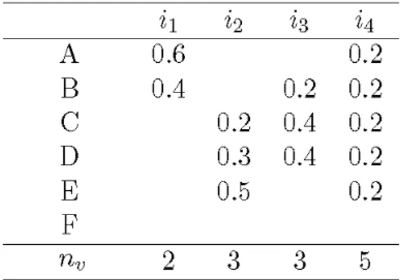
4.1 Membership values for six topics assigned by four individuals 40

5.1 Dataset with two different scales of noise 51

5.2 Two FADDIS-a clustering results forsca=0 using Gaussian Kernel pre-processed

with Lapin (5.2(a)) or without Lapin transformation (fig:faddisab0gk) 54

5.3 FADDIS-a AVG/STD plots for ARI 55

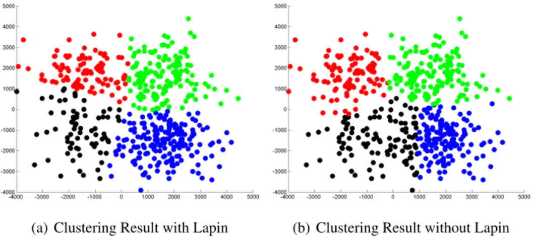
5.4 Two FADDIS-m clustering results forsca=0 with and without the Lapin

trans-formation 57

5.5 FADDIS-a AVG/STD plots for ARI 57

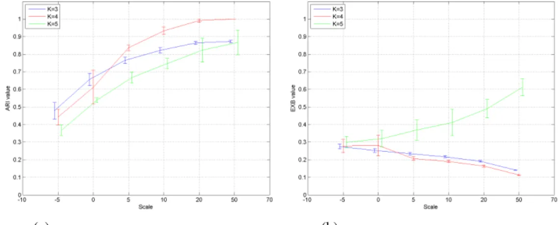
5.6 FastMap FCM avg/std plots for EXB and ARI 60

5.7 Three FMFCM clustering results forsca=0 andK={3,4,5} 60

5.8 NERFCM avg/std plots for EXB and ARI 62

5.9 Three NERFCM clustering results forsca=0 andK={3,4,5} 63 5.10 Three NERFCM clustering results forsca=0 andK={3,4,5} 64 5.11 VAT applied to a FCC generated dataset withK=3,N=200 andα =0 71

5.12 FADDIS-a plots forK=5 andN=200 for measures ARI, CEMR and REI 72

5.13 ARI avg/std plots for all algorithms forK=5 andN=400 75

(16)

5.14 Original Iris Dataset Classification 82

5.15 Iris Data Clustering Results for FADDIS with Gaussian Kernel 88

A.1 VAT tool results for each dataset for Conventional Proximity 98

A.2 FADDIS-a results for one example dataset for each scale value 100

A.3 FADDIS-a results for one example dataset for each scale value 101

A.4 FADDIS-m results for one example dataset for each scale value 102

A.5 FADDIS-m results for one example dataset for each scale value 103

A.6 FastMap FCM results for one example dataset for each scale value and K={3,

4, 5} 104

A.7 FastMap FCM results for one example dataset for each scale value and K={3,

4, 5} 105

A.8 NERFCM results for one example dataset for each scale value and K={3, 4, 5} 106

A.9 NERFCM results for one example dataset for each scale value and K={3, 4, 5} 107

B.1 FADDIS-a results withK=3 andN=50 114

(17)

B.16 FADDIS-m results withK=3 andN=50 124

B.31 FastMap FCM ARI mean/avg forK=3 134

B.34 NERFCM ARI mean/avg forK=3 138

B.35 NERFCM ARI mean/avg forK=5 139

(18)

C.1 Original Cancer Dataset Classification 142

C.2 Cancer Data Clustering Results for FADDIS with Gaussian Kernel 147

C.3 Original Wine Dataset Classification 149

(19)

5.1 FADDIS-a Most frequent Stop condition and Number of extracted clusters for

Gaussian Kernel (in 10 runs) 53

Gaussian Kernel with Lapin transformation (in 10 runs) 54

5.3 FADDIS-a ARI AVG/STD for Gaussian Kernel with and without the Lapin

transformation 55

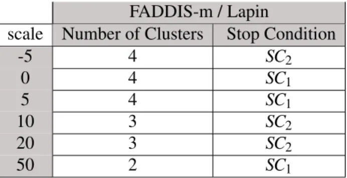
5.4 FADDIS-m Most frequent Stop condition and Number of extracted clusters for

Gaussian Kernel (in 10 runs) 56

Gaussian Kernel with Lapin transformation (in 10 runs) 56

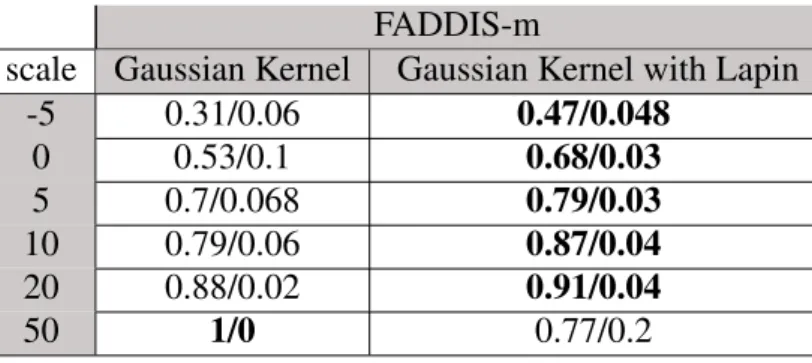
5.6 FADDIS-m ARI avg/std for Gaussian Kernel with and without the Lapin

trans-formation 58

5.7 Adjusted Rand Index avg/std for FastMap for each K 59

5.8 Extended Xie-Beni avg/std for FastMap for each K 59

5.9 Adjusted Rand Index avg/std for NERFCM for each K 61

5.10 Extended Xie-Beni avg/std for NERFCM for each K 62

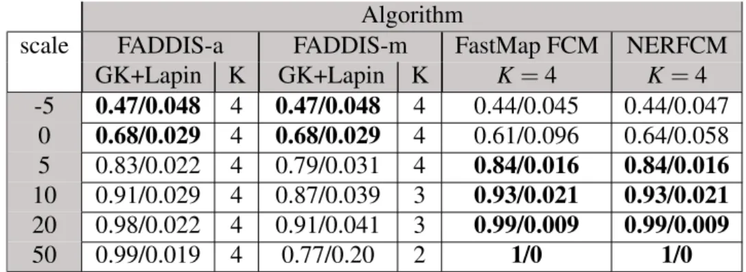
5.11 Adjusted Rand Index avg/std for all algorithms in best conditions and number

of extracted clusters Mode for FADDIS 64

5.12 Minimum contribution thresholdε fine tuning for each case for FADDIS-a 71

5.13 Minimum contribution thresholdε fine tuning for each case for FADDIS-m 71

5.14 Mode and Percentage avg/std of correct extracted clusters for std of Gaussian

noise=[0, 0.1] forK=5 73

(20)

5.16 REI avg/std for std of added Gaussian noise=[0, 0.1] for K=5 74

5.17 Summary Table for ARI avg/std for std of added Gaussian noise=[0, 0.1] for all

algorithms in best conditions for K=5 74

5.18 Crisp Core Matching (%) avg/std for std of added Gaussian noise=[0, 0.1] for

K=5 76

5.19 Summary Table for ARI avg/std for std of added Gaussian noise=[0, 0.1] for all

algorithms in best conditions forK={3,5,7} 77

5.20 Summary Table of Crisp Core Matching (%) avg/std for std of added Gaussian

noise=[0, 0.1] for all algorithms in best conditions forK={3,5,7} 78

5.21 FMFCM results for Iris Data 83

5.22 NERFCM results for Iris Data 83

5.23 Confusion Matrix Obtained from original classification and clustering results of

Iris Data with FADDIS-a using the Gaussian Kernel without Lapin 84

5.24 Values for the contribution of the data scatter and intensity of the extracted

clusters for FADDIS-a for the Iris Data using Gaussian Kernel without Lapin 84

Iris Data with FADDIS-m using the Gaussian Kernel without Lapin 85

clusters for FADDIS-m for the Iris Data using Gaussian Kernel without Lapin 85

Iris Data with FADDIS-a using the Gaussian Kernel with Lapin 86

clusters for FADDIS-a for the Iris Data using Gaussian Kernel with Lapin 86

(21)

clusters for FADDIS-m for the Iris Data using Gaussian Kernel with Lapin 87

5.31 Summary Table of all benchmark datasets for all algorithms in best conditions 89

B.1 Percentage of correct extracted clusters avg/std for std of added Gaussian noise=[0,

0.1] for K=3 109

B.2 Characteristic of the membership Error avg/std for std of added Gaussian noise=[0,

0.1] for K=3 109

B.3 Intensity Error avg/std for std of added Gaussian noise=[0, 0.1] for K=3 110

B.4 Crisp Core Matching (%) avg/std for std of added Gaussian noise=[0, 0.1] for

K=3 110

B.5 Summary Table for ARI avg/std for std of added Gaussian noise=[0, 0.1] for all

B.6 Percentage of correct extracted clusters avg/std for std of added Gaussian noise=[0,

0.1] for K=7 111

B.7 Characteristic of the membership Error avg/std for std of added Gaussian noise=[0,

0.1] for K=7 111

B.8 Intensity Error avg/std for std of added Gaussian noise=[0, 0.1] for K=7 111

B.9 Crisp Core Matching (%) avg/std for std of added Gaussian noise=[0, 0.1] for

K=7 111

B.10 Summary Table for ARI avg/std for std of added Gaussian noise=[0, 0.1] for all

C.1 FMFCM results for Cancer Data 142

(22)

C.3 Confusion Matrix Obtained from original classification and clustering results of

Cancer Data with FADDIS-a applying the Gaussian Kernel 143

C.4 Values for the contribution of the data scatter and intensity of the extracted

clusters for FADDIS-a for the Cancer Data using the Gaussian Kernel 144

Cancer Data with FADDIS-m applying the Gaussian Kernel 144

clusters for FADDIS-m for the Cancer Data using the Gaussian Kernel 144

Cancer Data with FADDIS-a with Lapin applying the Gaussian Kernel 145

clusters for FADDIS-a with Lapin for the Cancer Data using the Gaussian Kernel 145

Cancer Data with FADDIS-m with Lapin applying the Gaussian Kernel 146

clusters for FADDIS-m with Lapin for the Cancer Data using the Gaussian Kernel146

C.11 FMFCM results for Wine Data 148

C.12 NERFCM results for Wine Data 148

Wine Data with FADDIS-a using the Gaussian Kernel 150

clusters for FADDIS-a for the Wine Data using Gaussian Kernel 150

(23)

clusters for FADDIS-m for the Wine Data using Gaussian Kernel 151

Wine Data with FADDIS-a with Lapin using the Gaussian Kernel 152

clusters for FADDIS-a with Lapin for the Wine Data using Gaussian Kernel 152

Wine Data with FADDIS-m with Lapin using the Gaussian Kernel 152

clusters for FADDIS-m with Lapin for the Wine Data using Gaussian Kernel 153

C.21 FMFCM results for Fat Oil Data 154

C.22 NERFCM results for Cancer Data 155

C.23 Confusion Matrix Obtained from FRC classification and clustering results of

Fat Oil Data with FADDIS-a 156

clusters for FADDIS-a for the Fat Oil Data 156

Fat Oil Data with FADDIS-m 156

clusters for FADDIS-m for the Fat Oil Data 157

Fat Oil Data with FADDIS-a with the Gaussian Kernel 158

(24)

Fat Oil Data with FADDIS-m with the Gaussian Kernel 159

clusters for FADDIS-m for the Fat Oil Data with Gaussian Kernel 159

Fat Oil Data with FADDIS-a with Lapin and the Gaussian Kernel 160

clusters for FADDIS-a with Lapin for the Fat Oil Data with Gaussian Kernel 160

Fat Oil Data with FADDIS-m with Lapin and the Gaussian Kernel 161

clusters for FADDIS-m with Lapin for the Fat Oil Data with Gaussian Kernel 161

C.35 FMFCM results for Country Data 162

C.36 NERFCM results for Country Data 163

Country Data with FADDIS-a 164

clusters for FADDIS-a for the Country Data 164

Country Data with FADDIS-m 165

clusters for FADDIS-m for the Country Data 165

(25)

clusters for FADDIS-a for the Country Data with Gaussian Kernel 166

Country Data with FADDIS-m with Gaussian Kernel 167

clusters for FADDIS-m for the Country Data with Gaussian Kernel 168

Country Data with FADDIS-a with Lapin and Gaussian Kernel 168

clusters for FADDIS-a with Lapin for the Country Data with Gaussian Kernel 169

Country Data with FADDIS-m with Lapin and Gaussian Kernel 169

clusters for FADDIS-m with Lapin for the Country Data with Gaussian Kernel 169

C.49 FMFCM results for Microcomputer Data 171

C.50 NERFCM results for Microcomputer Data 171

Microcomputer Data with FADDIS-a 172

clusters for FADDIS-a for the Microcomputer Data 172

Microcomputer Data with FADDIS-m 173

(26)

Microcomputer Data with FADDIS-a with Gaussian Kernel 174

clusters for FADDIS-a for the Microcomputer Data with Gaussian Kernel 174

Microcomputer Data with FADDIS-m with Gaussian Kernel 175

clusters for FADDIS-m for the Microcomputer Data with Gaussian Kernel 176

Microcomputer Data with FADDIS-a with Lapin and Gaussian Kernel 177

clusters for FADDIS-a with Lapin for the Microcomputer Data with Gaussian

Kernel 177

Microcomputer Data with FADDIS-m with Lapin and Gaussian Kernel 178

clusters for FADDIS-m with Lapin for the Microcomputer Data with Gaussian

(27)

K Number of clusters 5

d Distance function 12

xi ith object attribute vector 12

X Object data matrix 12

N Number of entities 12

S Similarity matrix 13

D Dissimilarity matrix 13

R Relational matrix 14

uik Membership of objectito clusterk 19

U Membership matrix 19

V Prototype vector 20

m Fuzzyfication factor 27

µk Intensity of clusterk 41

Λ Eigenvalues matrix 41

ε Minimum cluster contribution threshold 45

τ Minimum residual scatter threshold 46

(28)

(29)

1.1 What is Clustering?

Clustering is considered to be a method of unsupervised learning. It is a technique used in

statistic data analysis, such as in machine learning [31], data mining [45], bioinformatics [51]

and image recognition [5]. It tries to find a structure in raw data, by creating subsets of similar

instances. These subsets are the clusters, which are groups of objects that are similar between

them given certain criteria and dissimilar to the ones from other clusters.

As an example of a clustering process, two figures are shown, the first is an unlabeled data

set, and the second is a result from a clustering algorithm.

(a) Unlabeled Data (b) Result of Clustering

Figure 1.1 Clustering Example

The Clustering main objective is to find the best grouping of the data. In order to achieve

this, some input data may be useful. There is a great range of clustering algorithms, each one

may give different solutions for the given set. The problem that emerges is to decide whether a

(30)

When analyzing raw data, i.e data for which there is no original classification to compare

results, many solutions must be taken under consideration and different algorithms may return

different groupings. For example, the following figure obtained from [34]:

Figure 1.2 Different Clustering Results

Given the unclassified data, it could be concluded at first sight that there are 2 clusters, but

there are other possibilities that can be better. Also, the structure of the grouping may be an

issue as the next figure, taken from [33], shows:

Figure 1.3 Different Clustering Results

As can be seen, many possible groupings do exist along with the number of clusters for the

(31)

must be taken into consideration when analyzing and clustering data, such as the data properties,

specialists point of view, etc.

Clustering can be proven to be useful in many fields, and some examples taken from [33]

are:

1. Marketing: grouping customer data

2. Biology: grouping animals and plants

3. Medicine: identifying diseases and their severity

4. Web Mining: grouping access patterns to determine user’s interests

5. Face Recognition: grouping similar patterns to identify faces in images

6. Crime Analysis: grouping similar patterns of crime scenes to identify certain areas with

a higher criminality risk

This work will focus on relational fuzzy clustering algorithms, as will be explained in the

next sections.

1.2 Problem Description and Context

There is a distinction between object data and relational data. Whereas object data is described

by an attribute-value representation (e.g. height and weight on an object), relational data

(32)

objects. Relational data emerges in applications like Web user profiling [44] and DNA

microar-ray experiments to characterize the expression of groups of genes in the presence of treatments

[6].

In the framework of the project “Computational Approach to Ontology Profiling of

Scien-tific Research Organizations” (PTDC/EIA/69988/2006), a more recent real world application

concerns the definition of fuzzy membership profiles of the research activities conducted in a

University department following the ACM-CCS taxonomy [29]. From an electronic survey tool

(ESSA- https://copsro.di.fct.unl.pt/), the researchers of an organization are asked to select up to

six topics among the leaf nodes of the ACM-CCS taxonomy and assign each with a percentage

which expresses the proportion of the topic in the total of the researcher’s activity. This

de-scribes the researcher’s activity fuzzy membership profile. From that, it is derived a similarity

matrix between research topics covered by the fuzzy profiles. Then, a research organization is

represented by clusters of ACM-CCS topics to reflect thematic communalities between

activi-ties of researchers or teams working on these topics. The Fuzzy ADDItive Spectral clustering

(FADDIS) method has been introduced by Mirkin and Nascimento [27][28], for this propose,

and will be the object of main investigation in this dissertation.

Relational fuzzy clustering and additive fuzzy clustering are two types of methodological

approaches for learning the structure of similarity between objects as groups that share common

properties, standing on different model and algorithmic strategies.

The proposed work will be applied to benchmark relational datasets, affinity data and

simu-lated data according to a new Data Generator developed for the Fuzzy Additive Spectral

Clus-tering Algorithm (FADDIS) model, proposed by Mirkin and Nascimento in [27].

The experiments that will take place in this dissertation will take into consideration the used

(33)

1.3 Main Contributions

The main goal of this thesis is to study, experimentally compare and analyse two families of

fuzzy relational clustering algorithms:

1. Parallel versions of Fuzzy Relational Clustering, where the clusters are simultaneously constructed in each iteration of the algorithm and the number of clusters K is an input parameter of the algorithms. In order to analyse the best number of clusters, validation

indices recently proposed in the literature [8][50] will be applied.

2. Sequential Additive Fuzzy Relational Clustering, where the clusters are iteratively defined one-by one until a composed stop condition holds, which allows to determine the number

of clusters.

The selected parallel versions of Fuzzy Relational Clustering algorithms are the Non-Euclidean

Relational Fuzzy C-Means (NERFCM) by Hathaway et al [21] and FastMap Fuzzy C-means

(FMFCM) by Brouwer [9]. The chosen sequential algorithms are two recent versions of the

Fuzzy Additive Spectral Clustering (FADDIS) algorithm due to Mirkin and Nascimento [28].

Two data generators have been constructed in order to study the effectiveness of former

clustering algorithms in recovering a cluster structure of generated data in the presence of noise.

More precisely, it had been developed a “Bivariate Normal Data Generator” with noise, and

the “Fuzzy Core Clusters Data Generator” having as input a similarity data matrix generated

according to the underlying FADDIS model with added Gaussian noise.

An extensive simulation study with data sets generated under distinct levels of noise from

distinct number of clusters and with different cardinalities, has been conducted. Particular

at-tention is given on the study of FADDIS own properties, and specific evaluation and validation

(34)

two new error measures have been introduced to evaluate specific properties of the FADDIS

algorithms, the Characteristic of the Error of Membership Recovery (CEMR) and the Relative

Error of Intensities (REI). In the case of FADDIS, the pre-processing of the data with or without

Laplacian Pseudo-Inverse (LAPIN) transformation is an object of analysis, as well as the ability

of the algorithm on finding the “natural number of clusters” by tuning its stop conditions. On

the other hand, the aspect of determination of the number of clusters in case of NERFCM and

FMFCM is evaluated by using recent validation indices proposed in the literature [49]. All the

algorithms have also been tested with real world benchmark data sets. In addition, the VAT

algorithm was implemented in order to visualise cluster tendency from relational data.

To the present case study, the data that will be subject of analysis will be:

• Datasets generated from the Bivariate Normal Data Generator with noise, as an extension

of the datasets generated in Brouwer’s previous work [9].

• Datasets generated from the Fuzzy Core Clusters Data Generator;

• Several benchmark datasets taken from the literature [12][55].

In all cases, a previous classification of the data is known. All benchmark datasets have been

clustered before using different algorithms and the generated data also has its labels generated.

The obtained results will give a better understanding of the algorithms behaviour under

different datasets and it will be verified that some datasets can be clustered with better results

(35)

1.4 Organization

This thesis is organized in the following way: Chapter 1 was a general introduction to

clus-tering, where the main goals and contributions of this dissertation were referred. Chapter 2

is an introduction to Relational Fuzzy Clustering, where the data format and the parallel and

sequential methods will be addressed. In Chapter 3, the studied Relational Fuzzzy Clustering

algorithms will be described as well as validation indices. Following in Chapter 4, the Spectral

Fuzzy clustering is introduced and the Fuzzy Additive Spectral Method presented. Finally in

Chapter 5, each one of the experimental studies will be described. The final conclusions and

future work are presented in Chapter 6.

Further results of the experimental studies can be found in the Appendices and will be

(36)

(37)

2.1 Introduction

A common type of clustering algorithms, the hard clustering methods, cluster data such that

each entity belongs only to one group. This way, results are crisp and no additional information

is given. Fuzzy clustering introduced by Bezdek [3] which will be subject of study in the

present work, clusters data in a way that each point has a membership value for each cluster.

This expresses the degree of inclusion of the entities to each cluster, and further analysis of

these can be conducted.

In a first stage, clustering general information gathering must be made. Analyzing the

Clus-tering algorithms behaviour and their mathematical application will give a better insight on what

is happening when the data is being processed.

To start this research, the initial data must be analyzed. There are numerous forms in which

data can be represented initially, and the adopted methods to treat this information will be

decisive in the outcome.

The initial observation data may appear in different formats, besides being either object

or relational data, it can be numerical, consist of strings, percentage, binary, etc.. Each case

must be treated in a different way, and even may have a specific method to be normalized and

transformed into a more generic set that can be analyzed and used by clustering algorithms.

To understand the data manipulation and treatment that is needed so that the algorithms can

be used, some pre-processing techniques will be studied and some used in implementations.

An essential base for the greatest part of the fuzzy algorithms is the Fuzzy C-Means (FCM)

(38)

One such important extension is the Non-Euclidean Relational Fuzzy C-Means (NERFCM)

due to Hathaway and Bezdek [21], where the relational data given as input does not have to be

Euclidean.

Another approach is using the FastMap method by Faloutsos [15] to create object data from

relational data. This method will be used since its implementation is linear and this constitutes

an efficient and fast algorithm that has great potential. The resulting object data will then be

used with the FCM.

It is important to note that the referenced algorithms belong to the family of algorithms

where the number of clusters is an input parameter, which can be an issue, since validation

techniques must be applied and the algorithm has to be run numerous times with different

values for that number. The determination of a good number of clusters is a well known and

still unresolved problem in cluster analysis.

A distinct approach, which constitutes the main focus of study is the Fuzzy Additive Spectral

method developed by Mirkin and Nascimento [27][28]. This method extracts clusters

sequen-tially, one at a time, until a composed stop condition is achieved. This way, the number of

clusters is not an input parameter of the algorithm but instead is provided, in a natural way, by

the algorithm.

2.2 Entity-Attribute and (Dis)Similarity Data

In the various clustering algorithms, the input data to be clustered may be in different formats. A

common data structure is the entity-attribute matrix, which is a result of describing each object

(39)

categorical as gender, country, color, week days or binary. In order to work on these, some

techniques must be used based on the knowledge about the data context. Usually the functions

to determine the similarity degree for each attribute are distinct since different criteria is needed

for the data evaluation.

The main objective is to work on a numerical matrix, where each row represents an object,

and each column stand for one attribute which has its own domain of possible values. Many

algorithms such as the FCM, receives as input matrices in this format.

In contrast, the relational data expresses how (dis)similar the objects are. Each entity is not

defined in terms of a range of attributes, rather all values express a result of comparing all objects

using certain criteria. It can either be done by specialists of the area, or can be determined using

specific similarity measures. Relational matrices can either express how similar or dissimilar

objects are. In a similarity matrix, its maximum value represents high affinity between the

objects while in dissimilarity matrices high values mean the opposite. The similarity matrix can

also be known as an affinity matrix because it expresses the affinity degree of the objects. A

dissimilarity matrix is usually represented as:

whered(i,j)is the dissimilarity between objectsiand j. As an example, a dissimilarity measure is the Euclidean distance, where higher values represent higher distance between instances,

therefore greater dissimilarity. The diagonal is composed by only zeros, since an object is not

(40)

The choice of the similarity or dissimilarity measure to construct a relational matrix is

deci-sive for the quality of the clustering result, which may be determined by validation indices, as

some will be mentioned in the current work.

The main type of data used in this work will be relational, either similarity or

dissimi-larity matrices. When applying the algorithms, if the given data is in entity-attribute form, a

(dis)similarity measure will be used to build a matrix of the desired format (see Section 2.2.1).

In the FastMap method the opposite will happen, since FCM receives as input a entity-attribute

matrix, an affinity matrix will be converted into that type of data.

2.2.1 Transforming Entity-Attribute Data to Relational Data

Object-Entity data as mentioned before, can be transformed into Relational data using different

measures. A well known method is the conventional proximity, that relies on the Euclidean

distances to generate a relational dissimilarity matrix:

Di j =d2(xi,xj), (2.1)

whered is the Euclidean distance andxiandxjare respectively theithand jth objects.

Another used method is the Gaussian Kernel [24], following previous work by Ng. et al

[23] and Hathaway et al [17]. Given an object-entityN×pmatrixX, whereN is the number of entities and pthe number of attributes, affinity similarity data can be obtained by:

Si j =e −d(_xi,_{x j})2

2σ2 , (2.2)

(41)

the objects influences the affinity matrixS. Following the founding papers from Ng et al [23] and Shi and Malik [41], the diagonal elements are made equal to zero. The 2σ2value is claimed

to be a user defined parameter. In the experiments conducted by Mirkin and Nascimento [29],

consistent results have been obtained forσ2=p/9 wherepis the number of attributes and after the features have been normalized by range.

There are many occasions when a relational matrix is given to analyse. Since the relational

clustering algorithms may receive as input a similarity or dissimilarity matrix, it may be useful

converting between each other depending on the given and the required data format. Two

exam-ples used by Davé and Sen [12] will be presented to achieve this, whereDandSwill represent, respectively, dissimilarity and similarity matrices.

• Converting by maximum value:

D=maxS−S (2.3)

• Converting by minimum value:

D=1/S−min 1/S (2.4)

In particular, the presented methods can be applied the same way to obtain a similarity from

a dissimilarity matrix.

2.3 Visualizing Clustering Tendency in Relational Data

A tool for Visual Assessment of Cluster Tendency (VAT) was developed by Bezdek and

(42)

gives the user a perception of the possible number of clusters and relative sizes. This method

re-organizes the columns and rows of the relational matrix according to the dissimilarities between

objects. As an example, two figures are displayed.

The expected output is a plot, where black areas mean strong similarities and white areas

great dissimilarities between objects.

For a given relational matrix, if we directly plot it grayscale, the resulting image is for

example 2.1(a). After applying the VAT tool to the dissimilarity matrix, the obtained figure is

2.1(b).

As can be analysed from the first figure, nothing can be concluded, but from the second one,

four clusters can be distinguished located in the diagonal of the matrix with darker grey colors.

This may indicate that the given dataset may have a structure of four clusters. The original

classified dataset has in fact four clusters, and its plot is in figure 2.2.

(a) Normal plot output (b) VAT plot output

Figure 2.1 Example for applying VAT

The method algorithm is explained following [7], where Ris the input relacional matrix,n is the number of entities.

1. Initialize:

(43)

Figure 2.2 Original Classified Dataset example

G={1,2, ...,n};

J1=J2= [];

P= [0, ...,0];

2. Select(i,j)∈argmax p∈G,q∈G

{Rpq} Set:

P(1) =i; J1={i};

J₂=G\{i};

3. For r=2, ...,n:

Select(i,j)∈ argmin p∈J1,q∈J2

{Rpq}

Set: P(r) = j; J1=J1∪ {j};

J2=J2\{j};

(44)

4. Using the reordered vector P, determine the new relational matrix R′with: R′_{i j}=R_P(i)P(_j), for 1≤i,j≤n.

5. Output the matrix as a greyscale image, where low values are darker and higher values are brighter.

2.4 Parallel versus Sequential Relational Fuzzy Clustering Algorithms

Each clustering method has an algorithm to group the given data. Two main approaches can

be distinguished among the algorithms presented in the scientific literature. Parallel clustering

algorithms require as input parameter the number of clusters to be given, therefore the data is

seen as a K-cluster structure and populated taking this assumption in consideration. On the other hand, in case of sequential clustering, the algorithm extracts clusters one by one in each

iteration of the algorithm, until a stop condition is reached whose threshold values may have to

be tunned.

In the present work the described clustering algorithms are the following: the Fuzzy

C-means (FCM), Non-Euclidean Relational Fuzzy C-C-means (NERFCM), FastMap FCM

(FM-FCM) and the Any Relational Clustering Algorithm (ARCA). As for the studied sequential

clustering algorithms, they will be the Relational Fuzzy Subtractive Clustering (RFSC) and the

Fuzzy Additive Spectral Method (FADDIS).

There are several sequential clustering approaches, such as the one by Ott et al [36] or

Urahama et al [14]. It usually starts with the selection of some similarity measure to build an

(45)

or number of clusters is known. The main objective of a clustering algorithm is to extract the

best clustering solution from the data.

Each of the clustering algorithms has its own advantages, but not all have these items in

consideration. Most algorithms fail when the dataset has clusters with different shapes, like the

Sequential extraction of fuzzy clusters using a spectral graph by Inoue and Urahama [22], where

only Gaussian distributed data can be clustered correctly. Also, even when choosing from the

best similarity measures and attributes to represent the data, some algorithms are unable to find

acceptable results as mentioned before.

2.5 The Problem of the Number of Clusters

The determination of the number of clusters for a given dataset has been and still is a big

is-sue in the clustering community. New and raw data is always a challenge to clustering since

no additional information is known in most cases, leading to a number of clusters problem.

In these cases, an expert intervention is crucial when available, as a range of number of

clus-ters can be obtained. Having this, the algorithms can be applied as many times as the size

of that range, and then the quality of clusters and clustering analyzed using validation indices

[16][35][47][49][50].

As for the sequential clustering algorithms, the number of clusters is not needed as input

parameter, but some information about the data is, since a stop criterion usually needs to be

tuned. The same is applied in these cases, modifying the parameters and the stop criteria,

various results may be obtained and therefore analysed and validated in order to select the best

combination of values and cluster structure.

(46)

based on which index and algorithm are used. Having this, the number of clusters is again the

main issue.

With this in mind, the practical results and analysis in this work will compare results from

(47)

3.1 Introduction

This chapter presents several algorithms of Relational Fuzzy Clustering. First, Fuzzy C-means

(FCM) will be presented since some algorithms are either extensions or use it in their

compu-tation. Following, four relational fuzzy clustering algorithms will be introduced, two of which

will be used in the practical experiments. Finally, some validation indices will be applied to

evaluate the quality of fuzzy partitions, in particular validation indices to determine the best

number of clusters from relational clustering will be described.

3.2 Fuzzy C-Means

The Fuzzy C-Means by Bezdek [4] is a reference algorithm for the clustering community. Based

on object-feature data, the method determines subsets that will constitute the clusters. The

num-ber of generated clusters is an input variable to the algorithm. The FCM algorithm converges,

at least along a subsequence, to either a local minimum or saddle point of the FCM objective

function as presented by Hathaway et al in [19].

The produced membership matrixU ∈Rc×n, where _c is the number of clusters and _nthe number of objects. Eachuikis the degree that the objectOkbelongs to clusteri. Also, the matrix U will be under the following constraints:

1. uik∈[0,1], 1≤i≤c,1≤k≤n

2. ∑c_i=₁uik=1, 1≤k≤n

(48)

3. ∑n_k=₁uik>0, 1≤i≤c

The Fuzzy partitioning allows each object total membership to be distributed through all

clusters. The algorithm assumes that the clusters all circular shaped, and will determine their

centersvi, prototypes.

The algorithm will be described then as:

1. Initialize: Select an initial partitionU0that obeys the constraints mentioned above, startup a prototype matrix V = [v1, ...,vc]∈Rc×n, c is the input number of clusters, n is the number of objects, and select a fuzzyfication factor m≥1 and a k·k, that is any inner

product norm. A stop criterion ε must be defined as well as the number of maximum

iterations for the algorithm,r=1...rmax.

2. Update distances:

v(r)_i = ∑

n

k=1(u(r)ik )mxk

∑n_k=₁(u(r)_ik )m 1≤i≤c (3.1)

(d_ik(r))2= xk−v

(r) i 2

1≤i≤c,1≤k≤n (3.2)

3. Update partition:

For each object k=1...n,

if d_ik(r)>0, for i=1...c

u(r+_ik 1)=



 c

∑

j=1

(d_ik(r))2 (d(r)_jk )2



 −_m1₋₁

(3.3)

(49)

u(r+_ik 1)=0 ifd_ik(r+1)>0, whereu(r+_ik 1)∈[0,1]and

c

∑

i=1

u(r+_ik 1)=1 (3.4)

4. Convergence check: Ifr=rmax or|u(r+1)−u(r)|<ε stop the algorithm, otherwise go

to step 2 of the algorithm withr=r+1.

3.3 Non-Euclidean Relational FCM (NERFCM)

The Relational Fuzzy C-means (RFCM) is a relational dual of fuzzy c-means, following

Hath-away et al in [20] and [18]. The FCM as mentioned before is an algorithm that uses as input

object-feature data and RFCM appears as an extension of FCM to relational data. the

Non-Euclidean Relational FCM by Bezdek et al [21], is an extension for RFCM, works as a

safe-guard, since relational data may not be Euclidean, and applying aspreadingtransformation, the algorithm works as expected in these cases as well.

Some modifications to the original FCM will be made to achieve this. A relational matrixR is given as input, thats is defined as

Ri j = xi−xj

2

1≤i,j≤n, (3.5)

wherenis the number of objects. The second step formulas in FCM will be changed for:

v(r)_i =

h

(U_i(r)₁ )m...(U_in(r))miT

(50)

(d_ik(r))2= (Rv(r)_i )k− 1 2(v

(r) i )

T_R₍_v(r)

i ) 1≤i≤c,1≤k≤n. (3.7)

Using these equations in the second step, RFCM is obtained. In order to build a

non-Euclidean resistant algorithm, some modifications must be made. The transformation consists

in the addition of a positive numberβ to all off-diagonal elements ofR. The new matrixR_β can be defined as:

(Rβ)jk=       

Rjk+β, if j6=k 0, if j=k

. (3.8)

IfRis a relational matrix, but not Euclidean, then there exists a positiveβ0such thatRβ is

Euclidean for allβ ≥β0and not Euclidean forβ <β0. Calculating the exact value forβ0could

be very expensive computationally, but an overestimation could lead into data loss as well, so

the method will calculate values forβ in each iteration.

The changes that need to be made to FCM will be adding the initialization parameterβ =0

to the first step, and replacing the second with:

v(r)_i =

h

(u(r)_i₁ )m_...₍_u(r) in )m

iT

∑n_k=₁(u(r)_ik )m 1≤i≤c, (3.9)

(d(r)_ik )2= (Rβv(r)i )k− 1 2(v

(r) i )

T

Rβ(v(r)i ) 1≤i≤c,1≤k≤n. (3.10)

(51)

△β =max     

−2(d_ik(r))2

v

(r) i −ek

2      (3.11) and modify

(d_ik(r))2←(d_ik(r))2+△β

2 v

(r) i −ek

2

1≤i≤c,1≤k≤n, (3.12)

updatingβ value

β ←β+△β. (3.13)

In the mentioned formulasekis thekth unit vector inRn. The NERFCM will be a reference method in the present work.

This algorithm has been applied with successful results within many datasets. Examples of

such data in bioinformatics, are the gene similarity matrices obtained from using Basic Local

Alignment Search Tool (BLAST) by Altschul et al [1][54] and Gene Ontology [53] similarities

in a dataset of 194 human genes, following Popescu et al [38].

3.4 FastMap FCM

This method, by Brouwer [9], starts by using the Fast Map algorithm [15] on given data to

produce points in the Euclidean space so that it can be visually analysed and FCM [4] applied.

Visual clustering allows a better understanding and analysis of the obtained results and a

(52)

further. This visualization maps the objects preserving their proximity relationship. The

pro-duced data will bek-dimensional, wherekis an input parameter, and the selected algorithm to use on the result is the FCM.

3.4.1 FastMap Method

The FastMap method maps data into points in a k-dimensional space, preserving their

dissim-ilarities. This method is quite fast, since its implementation is linear. The only input is the

dissimilarity matrix, that should be Euclidean, even though the method works if it is not. Given

a matrix withnobjects and their distance information, the method will find some othernobjects but in ak-dimensional space such that the distances are maintained.

This is achieved by creating an axis from 2 well separated objects, Oa and Ob. With this, the projections of each object using this axis, can be given in terms of the Dissimilarity matrix

D:

xi=

D2_a_,_i+D_a2_,_b−D2_b_,_i 2∗Da,b

, (3.14)

and the distance between the object projections in the reduced space:

D′2_i_,_j=D2_i_,_j−(xi−xj)2 i,j=1...n, (3.15)

wherenis the number of objects, and i,j are 2 object indexes. The idea is to project thenobjects on k mutually orthogonal directions. The main difficulty is to achieve this with only one input,

(53)

3.4.2 Describing the method

First, 2 pivot objects must be chosen in order to generate an axis on the k-dimensional space.

choose-distant-objects(O,D

1. Choose a random object as second pivotOb

2. SetOaas the farthest object fromOb

3. SetObas the farthest object fromOa

4. ReturnOa,O_b

Having this function, the algorithm for FastMap can be presented as follows:

FastMap:

beginGlobal variables:

Nxkmatrix X In the end, the i-th row is the projected i-th object 2 xkpivot array PA Array of pivot objects for each iteration

int col = 0; Current X column being updated

FastMap(k,D,O) 1)ifk≤0thenend;

elsecol+ +; fi

2)choose pivot objects

(54)

3)put pivot object ids in PA

Pa[1,col] = a;

Pa[2,col] = b;

4)ifD(Oa,O_b) =0

then fori:=1ton

doX[i,col] =0; end; od fi

5)Project all objects on the axis formed byOaandOb

fori:=1tondoX[i,col] =compute (3.14); od

6)ComputeD′from (3.15) callFastMap(k−1,D′,O)

After constructing the k-dimensional object data, the FCM algorithm is then applied as

usual.

This algorithm is quite recent and not yet many studies have been made, but some

experi-ments were made with randomly generated matrices by Brouwer in [9]. All the matrices were

clustered using different algorithms and FMFCM returned better results in many cases. Being

an interesting method to analyse, this algorithm will be implemented and used in experiments

(55)

3.5 Any Relation Clustering Algorithm (ARCA)

The Any Relation Clustering Algorithm (ARCA) by Corsini et al [11], is based on the FCM

algorithm and is claimed by the authors to outperform the NERFCM method [21]. In ARCA,

each datum is represented by a vector of its relation strengths to the other objects of the data

set and the prototype is an object that may not exist in the data set, and its relationship with all

the objects is representative of the mutual relationships of a group of datum with high

similar-ity. The algorithm starts by partitioning the dataset minimizing the euclidean distance between

objects and the prototype of the cluster.

This partitioning is obtained by minimizing:

Jm(U,V) = C

∑

i=1 N

∑

k=1

um_i_,_kδ2(xk,vi), (3.16)

whereCis the number of clusters,N is the number of objects,xiis an object,vi is a prototype, ui,k is the membership degree of objectxkto the cluster with prototypevi,mis the fuzzyfication factor and δ(x_k,vi) is the deviation between the relation of xk and the other objects and the relation ofviand the other objects. δ is defined as:

δ(xk,vi) = s

N

∑

s=1

(rk,s−vi,s)2, (3.17)

where rk,s is the relation between xk and xs, and vi,s is the relation between the prototype vi andxs. Using the Lagrange multipliers [46] minimization method, the ARCA algorithm can be defined as:

1. DefineCas 2≤C<N, 1<m<∞, and choose an initial partition U(0).

(56)

(a) calculateV(l) = [v(l)_i_,_k]:

v(l)_i_,_k = ∑

N s=1um

(l) i,k rk,s

∑N_s=₁um_i_,_k(l) (3.18) (b) updateU(l)toU(l+1):

u(l+_i_,_k 1)=



 C

∑

j=1

δ(xk,vi)(l) δ(xk,vj)(l)

!_m₋2₁

 −1

(3.19)

(c) if U(l+1)−U(l)<ε then stop, else continue iteration and restart step 2 with l=l+1

This algorithm has been applied to 4 benchmark datasets (Fat Oil Data, cat cortex, proteins

and Tamura dataset) and 4 synthetic relational generated datasets in work by Corsini et al [11].

The algorithm returned good results in most cases according to the validity indices used by the

authors.

3.6 Relational Fuzzy Subtractive Clustering (RFSC)

The algorithm, as described by Suryavanshi et al [43], receives as input a relational matrixR, where Ri j is the similarity or dissimilarity between datum xi and xj. Ri j ≥0, Ri j =Rji and Rii=0. The algorithm starts by obtaining the potential of being a center cluster of each object, using:

Pi= NU

∑

j=1

e−αR2i j_, (3.20)

(57)

α =4/γ2, (3.21)

where NU is the total number of points to be clustered and γ is calculated as follows. Each objectihas a neighbourhood-dissimilarity value γi, which is the median of dissimilarity to all other objects. The neighbourhood-dissimilarity for the datasetγ is the mean of the various γi,

for eachi. The object with the highest potentialP₁∗ is then extracted as the first cluster center, and the potential of other objects is reduced proportionally to the similarity to the extracted

center. It is trivial to note that the potential of objects that are nearer to the extracted center

will be reduced more than the ones that are farther away. After this, the next cluster center will

be obtained from the next highest potential object, xt, withPt∗, as it will be a potential cluster center. At this point 2 thresholds have to be set, the accept ratioAand the reject ratioF, having 0<A,F<1 andF<A. With this we can decide if the extracted object will be a cluster center:

1. If Pt >AP₁∗, then xt is selected as the next cluster center and the subtractive method repeats.

2. IfPt<FP1∗, thenxt is rejected and the algorithm stops.

3. IfFP₁∗<Pt<AP₁∗, then the potential is said to have fallen in the gray region, and if the object offers a good trade-off between its potential and distance from the existing clusters

then it is accepted as the new cluster center.

This process continues until the item 2 is verified, which is the termination condition.

Af-ter this, C cluster centers were found, and the memberships of each object to each cluster is determined with:

ui j=e−αR 2

(58)

wherei= [1..C],j= [1..N]andRcijis the dissimilarity of thei

th_{cluster center with object}_x_{j. If} xj=xcij, thenRcij=0 and the membershipui j =1. Unlike the fuzzy c-means, RFSC relaxes

the constraint∑C_i=₁ui j =1, which makes it less sensitive to noise.

A cluster validity index can then be used to measure the quality of the clustering. In general

good clustering provides high inter-cluster distance values and low intra-cluster distance values.

The defined validity measure for the RFSC algorithm uses a ratio between the compactness to

the separation of clusters. The compactness is obtained as follows:

Compactness=

C

∑

i=1

∑N_j=₁u2_{i j}R2_c_i_j ∑N_j=₁ui j

!

/C (3.23)

As for separation, it is calculated as:

Separation=mini6=kR2cick, (3.24)

whereRcick is the dissimilarity between cluster centersciandck.

The index is obtained as:

Index o f goodness=Compactness

Separation (3.25)

The best clustering is found using the accept ratioAand the reject ratioF such that the index of goodness finds its minimum value.

Some experiments were conducted with user access logs from the web server of Computer

Science and Software Engineering Department (CSE) at Concordia University by Suryavanshi

(59)

3.7 Validation Indices

Clustering validation does not only entail the analysis of the best number of clusters, but also the

quality of the clustering partition and of each cluster itself. These indices express how ”good”

are clusters in a dataset, based on geometric or statistical properties according to a predefined

meaning of good clusters.

Validity indices can be used having different perspectives:

• When analyzing only the resulting membership matrixU, the validity index measures the quality ofU in terms of how the partitioning reveals a substructure.

• Having initial information, an index can be used to measure how a clustering algorithm

can recover the original cluster structure.

Applying validity measures usually constitutes a problem in the clustering community, since

no matter how good an index may be, there is always a dataset for which it will not give

accept-able results. There is no best measure to be used with all algorithms and data structures. In order

to bypass this problem, it is suggested according to Bezdek et al [5] to apply different validation

measures and select the best value among the results. Even though this approach can be more

accurate, it may still fail due to the various reasons already referred. The best strategy is to use

many different parameters when applying the clustering algorithms and use various indices. If

the procedure leads to consistent results, then it can be assumed that an acceptable structure was

found, otherwise more simulation has to be done before taking under consideration any results.

Some validation indices were studied and will be implemented to compare results of

clus-tering and cluster quality using different relational clusclus-tering algorithms. When using parallel

clustering algorithms, a range of values for the number of clusters is usually applied to analyse

(60)

used as a criterion in the various data sets, as some algorithms return better results than others

depending on the used data set.

In the next sections some indices that were used by Brouwer [9] will be presented. Some

approaches for cluster validity can be found in the list by Bezdek [?].

3.7.1 Roubens

The measure proposed by Roubens [39] (and also Bezdek [2]) only requires the resulting fuzzy

membership matrix obtained from the clustering algorithm, and the value represents how close

it is to being crisp. The method is

VR=

∑np_p=₁∑nk_k=₁(Mn,p)2

np , (3.26)

where M is the fuzzy membership matrix, np is the number of objects and nk the number of clusters. The closer this value is to 1 the more crisp are the results and if the value is closer to 0

it means the resulting matrix is fuzzier.

3.7.2 Rand Index and Adjusted Rand Index

In order to compare clustering results with some already existent ones, a measure of agreement

of partitions memberships is needed. Given two partitions: U being the original classification andV the clustering result, both composed by the objects from the set S=o1,o2, ...,on, the

(61)

Figure 3.1 Contingency table example

Forox,oy∈S, the Rand Index (RI) according to Yeung and Ruzzo [50] can be calculated by:

RI= a+d

a+b+c+d, (3.27)

where

1. ais the number of pair of objects(ox,oy)such that both belong to the same cluster in both sets of results.

2. b is the number of pair of objects (ox,oy) such that both belong to different clusters in both sets of results.

3. cis the number of pair of objects(ox,oy)such that both belong to the same cluster in the

first set of results and belong to different clusters in the second set.

4. cis the number of pair of objects(ox,oy)such that both belong to the same cluster in the second set of results and belong to different clusters in the first set.

The result obtained from this index will be in the interval[0,1]and is best when closer to 1.

(62)

ARI=

∑i j n₂i j

−∑i(ai₂)∑j(b j₂) (N

2)

1 2

h ∑_i ai

2

+∑_j bj

2

i

−∑i(ai2)+∑j(b j₂) (N

2)

, (3.28)

whereN=∑c_i=₁bi+∑r_j=₁aj.

As the RI, ARI takes its values from the interval[0,1]and the best result corresponds to the

maximum value.

3.7.3 Extended Xie-Beni Fuzzy Validity Index

This index appears as an extension to the well known Xie and Beni validity measure [49], which

takes under consideration the separation and compactness of clusters in a fuzzy c-partition. This

is expressed as a ratio of the intra-cluster scatter and minimum inter-cluster distance.

The presented index consists of a relational version of the Xie and Beni measure, introduced

by Bezdek et al [8]. This technique determines the cluster prototypes, used to calculate the

index, as

pj=argmax

1≤k≤n (

n

∑

i=1

um_j_,_i·rk,i )

, j∈N₁_,_c_, (3.29)

where pj is the index to the object that represents the jth prototype,mthe fuzzification factor, uj,i is the membership of the ith entity for the jth cluster from the membership matrixU and rk,i is the affinity value between thekth andith entities from the relational data matrix R. The relational Xie-Beni validity index can then be computed as

VRX B= ∑

n

i=1∑cj=1umj,i·rpj,i

n·min

j6=k

rpj,pk

(63)

As the resulting value decreases, the clustering quality increases according to this validity

(64)