João Luís Rodrigues Fernandes
Analysis of Classification Algorithms for Crop
Detection using LANDSAT 8 images
Dissertação para obtenção do Grau de Mestre em Engenharia Informática
Orientadores: Carlos Viegas Damásio, Prof. Associado, Universidade Nova de Lisboa
Susana Nascimento, ProfaAuxiliar, Universidade Nova de Lisboa Adélia Sousa, ProfaAuxiliar, Universidade de Évora
Júri:
Analysis of Classification Algorithms for Crop Detection using
LANDSAT 8 images
Copyright cJoão Luís Rodrigues Fernandes, Faculdade de Ciências e Tecnologia, Universidade Nova de Lisboa
A
CKNOWLEDGEMENTS
To my advisers, thank you all for the help, support and feedback throughout the year. To my friends and family, thank you for the continued support and availability. All of you were essential in helping me do this work.
A
BSTRACT
Remote sensing - the acquisition of information about an object or phenomenon without making physical contact with the object - is applied in a multitude of different areas, ranging from agriculture, forestry, cartography, hydrology, geology, meteorology, aerial traffic control, among many others. Regarding agriculture, an example of application of this information is regarding crop detection, to monitor existing crops easily and help in the region’s strategic planning.
In any of these areas, there is always an ongoing search for better methods that allow us to obtain better results. For over forty years, the Landsat program has utilized satellites to collect spectral information from Earth’s surface, creating a historical archive unmatched in quality, detail, coverage, and length. The most recent one was launched on February 11, 2013, having a number of improvements regarding its predecessors.
This project aims to compare classification methods in Portugal’s Ribatejo region, specifically regarding crop detection. The state of the art algorithms will be used in this region and their performance will be analyzed.
Keywords: land cover, remote sensing, landsat, classification, crop detection
R
ESUMO
Detecção remota - a aquisição de informação sobre um objecto ou acontecimento sem efectuar contacto físico com o objecto - é aplicada numa grande variedade de áreas, desde agricultura, engenharia florestal, cartografia, hidrologia, geologia, meteorologia, controlo de tráfego aéreo, entre muitas outras. Dentro da agricul-tura, um exemplo de aplicação destes dados é relativo à detecção de culturas, para monitorizar as culturas existentes de forma fácil e ajudar no planeamento estratégico de regiões.
Em qualquer destas áreas, existe sempre uma busca por melhores métodos que por sua vez permitam obter maiores resultados. Por mais de quarenta anos, o programa Landsat utilizou satélites para recolher informação espectral da super-fície terrestre, criando um arquivo histórico inigualável em qualidade, detalhe, cobertura e duração. O mais recente satélite foi lançado em 11 de Fevereiro de 2013, tendo algumas melhorias relativamente aos seus antecessores.
Este projecto tem como objectivo comparar métodos de classificação na área do Ribatejo, mais especificamente relativo à detecção de culturas, utilizando os algoritmos mais avançados e analisando o seu desempenho.
Palavras-chave: cobertura terreste, detecção remota, landsat, classificação, detec-ção de culturas.
C
ONTENTS
Contents xiii
1 Introduction 1
1.1 Problem Description . . . 6
1.2 Approach . . . 6
1.3 Main Contributions . . . 6
1.4 Document Organization . . . 7
2 Related Work 9 2.1 Spectral Signatures . . . 9
2.2 Sensor/Platform Systems . . . 12
2.2.1 Photography . . . 12
2.2.2 Satellite-Based Systems . . . 13
2.2.3 Landsat . . . 14
2.3 NDVI . . . 16
2.4 Image Correction . . . 17
2.5 Land Cover Classification Methods . . . 18
2.5.1 Algorithm Comparisons for Land Cover Applications . . . . 20
2.5.2 Pixel-based Classification versus Object-based Classification 21 2.5.3 K-Nearest Neighbor . . . 24
2.5.4 Decision Trees . . . 25
2.5.5 Random Forests . . . 26
2.5.6 Support Vector Machines . . . 27
2.5.7 Maximum Likelihood . . . 28
2.6 Evaluation Measures for Data Classification . . . 29
2.6.1 Cross-validation . . . 29
2.6.2 Confusion Matrix . . . 30
2.6.3 Cohen’s Kappa coefficient . . . 31
2.7 Used Technologies . . . 32
2.7.1 R Packages . . . 32
2.7.2 Shapefiles . . . 33
2.8 Summary . . . 34
3 System development 35 3.1 Preliminary Work . . . 35
3.2 Approach . . . 35
3.3 System Information/Results Replication . . . 37
3.3.1 Folder structure . . . 37
3.3.2 Result replication . . . 39
3.4 Data Preparation . . . 39
3.4.1 Shapefile Preparation . . . 40
3.4.2 Layers Preparation . . . 42
4 Experimental Study 43 4.1 Work Phases . . . 43
4.1.1 Single-image phase . . . 43
4.1.2 Multi-image phase . . . 45
4.2 Single-image phase . . . 46
4.2.1 Pre-Classification . . . 46
4.2.2 Classification . . . 50
4.2.3 Complementary studies . . . 55
4.3 Multi-image phase . . . 61
4.3.1 Random Forest Classification . . . 61
4.3.2 Support Vector Machine Classification . . . 64
4.3.3 Images . . . 66
4.4 Single-image phase discussion . . . 68
4.5 Multi-image phase discussion . . . 72
5 Conclusion and Further work 73
Bibliography 77
A List of R packages in the system 83
B 2015 images’ confusion matrices 87
C
H
A
P
T
E
R
1
I
NTRODUCTION
Remote Sensing can be defined as the process in which information is recorded/ob-served/perceived about an object, area, phenomenon or event without being in actual contact with them - the art or science of telling something about an object without touching it (Fischer et al. (1976)).
In modern usage, the term usually refers to the use of aerial sensor technology to detect and classify objects both on Earth itself and its atmosphere, using electro-magnetic radiation reflected or emitted from the earth’s surface (Campbell (2002)). It may be split into active remote sensing - when the energy measured is provided by the sensors themselves (e.g. RADAR systems), and passive, measuring ambient levels of existing sources of energy, such as sunlight.
The majority (but not all) of remote sensing is done with passive sensors, in which the sun is the major energy source (Eastman (2003)). Photography is the earliest example of this, capturing the reflection of light off earth features. Although photography is still a major part of remote sensing, newer technologies have been developed to capture wavelengths outside of the visible spectrum, such as ultraviolet and infra-red.
Land Cover is the physical material at the surface of the earth. Land covers in-clude asphalt, grass, trees, water, soil, among many others. Land cover is inherently subject to indeterminacy and relativism, since the meaning of certain classifica-tions can be defined in different ways. For example, in the United Kingdom, areas without trees may be sometimes classified as forest if there is intention to replant, while in Scandinavia areas with slow-growing trees might not be considered forest at all (Comber et al. (2005)).
There have been multiple attempts to define a standardized classification system, a system able to describe the complete range of land cover features independent of the scale or means used to map, such as the Land Cover Classification Sys-tem (Di Gregorio (2005)) or the various MODIS - Moderate Resolution Imaging Spectroradiometer - datasets (MODIS), among others.
Crop Detection can be defined as the detection/monitorization of crops and crop types in agricultural land. This process can greatly benefit land owners by providing information about issues such as drought, pest infestation, detecting water stress in crops, among others, and this information may help in strategic planning regarding the area.
Remote Sensing has a growing relevance in the modern information society. It represents a key technology used in a multitude of different areas. The technological world evolves every day, both in theoretical and practical applications -the development of better algorithms, software and hardware allows us to obtain better and faster results for whichever tasks we do.
An area that can benefit from the use of remote sensing is crop detection -identifying/monitoring agricultural crops - can greatly benefit their owners. A number of applications for crop detection exist, such as:
Crop Rotation
Crop rotation is the practice of growing a series of different types of crops in the same area in sequential seasons. Detecting appropriate crop rotation practices can be facilitated by crop detection.
Pest Prevention
Pest infestations are an important issue in agriculture, by having information about crops, these can be prevented or at least contained in an easier way.
Loan Control
Loans can be provided for farmers planning to grow certain crops. Crop detection can also be used by the loan providers to confirm farmers applied the money as agreed.
Strategic Planning
A number of strategic decisions can be improved by crop detection, such as estimating areas, future crop productions, scheduling the collection of those crops, among others.
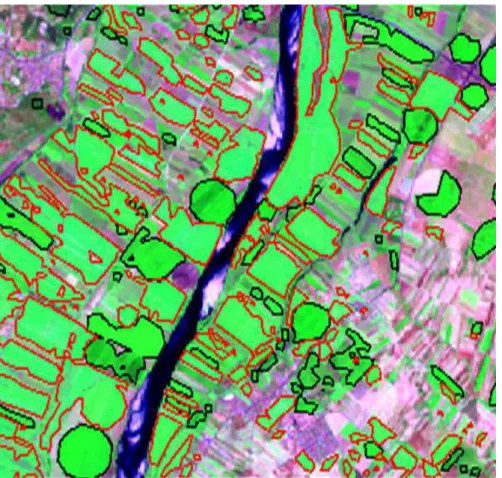
By applying remote sensing techniques, improvements such as lower costs, faster results and higher result accuracy can be achieved. Figure 1.1 shows an example of the final results of this, with landsat 5 images. The land is classified and the results of this are displayed to the user.
Figure 1.1: Simple crop identification. Red border is tomato, Black border is maize SourceProf. Adélia Sousa
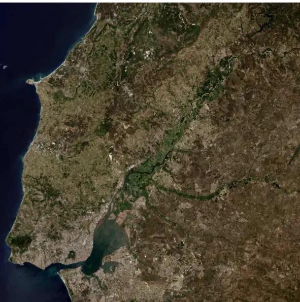
Region of study The Worldwide Reference System (WRS) is a global notation used in cataloging Landsat data. It enables a user to inquire about satellite imagery over any portion of the world by specifying a nominal scene center designated by PATH and ROW numbers. The WRS has proven valuable for the cataloging, referencing, and day-to-day use of imagery transmitted from the Landsat sensors. Both Landsat 8 and 5 (and others) follow the WRS-2. The combination of a Path number and a Row number uniquely identifies a nominal scene center. The Path number is always given first, followed by the Row number. The notation 127-043, for example, relates to Path number 127 and Row number 043.
Figure 1.2: The study area. Image generated by combining Landsat 8 bands 2, 3 and 4 (Blue, Green and Red).
The study will be done in the Ribatejo Province area, the most central of the traditional provinces of Portugal, with both no coastline or border with Spain. This region is crossed by the Tagus River, and contains some of the nation’s richest agricultural land, making it a relevant area to study. Existing crop types in the area include potato, vineyard, rice, tomato, maize, carrot, among others.
1.1
Problem Description
In any scientific area, there is always a search for methods that can improve the accuracy of results or facilitate their acquisition, and remote sensing is no different. Currently, detecting crops is a time-consuming procedure that is achieved by ground visits that cover a smaller area than necessary and as such, may deliver inconsistent results.
Previous work in the crop detection field, in the same study area as this work, was done by Prof. Adélia Sousa to classify small land portions. This was done with a single classification method and Landsat 5 imagery. We aim to extend this work by using Landsat 8 images, more classes and multiple classification methods, as described briefly in the following section and extensively in Section 3.2.
1.2
Approach
As mentioned before, remotely sensed data can be used to significantly lower costs, speed up results and improve the reliability of these results. A system was developed where the currently best regarded techniques of land cover classifica-tion could be compared, including tuning certain parameters of each algorithm. This system provides information regarding classification accuracy, and allows for full images of classified classes to be generated. It also allows for using images from different dates in the training and testing process. Although this is a brief description, a detailed section regarding the specifics of this approach is available on Section 3.2.
1.3
Main Contributions
1.4. DOCUMENT ORGANIZATION
1.4
Document Organization
In addition to this introductory chapter, the rest of the document is organized as follows:
Related Work
In chapter 2 we address some topics such as the mechanisms behind remote sensing, the classification methods, some classification evaluation measures, the technologies used in this work and the relevant literature.
System Development
In chapter 3 we describe extensively the approach taken, development of the created system for classifying images, the preliminary work done, how results can be replicated, and how the data was prepared.
Experimental Study
In chapter 4 the work phases performed are described, and the obtained results for the performed work are presented, along with discussion of these results.
Conclusion and Further Work
In chapter 5 the conclusion for this work is presented, and further work that could be done as an extension of the developed approach is described.
C
H
A
P
T
E
R
2
R
ELATED
W
ORK
In this chapter, some concepts related to the mechanisms behind remote sensing are explained, the classification methods are described, along with other relevant concepts to the classification evaluation. There is also mention of the technologies used in this work, and of the relevant literature.
2.1
Spectral Signatures
When electromagnetic energy strikes a material, the interaction that follows is reflection, absorption and/or transmission. Remote sensing uses the reflected portion as data, since this is the portion returned to the sensor system. Exactly how much is reflected will vary and will depend upon many factors such as the nature of the material and where in the electromagnetic spectrum the measurement is being taken.
If we look at the measurements of this reflection over a range of wavelengths, we get a spectral response pattern. A spectral response pattern, often called a signature, is a description of the degree to which energy is reflected in different regions of the electromagnetic spectrum, displayed often in the form of a graph.
Figure 2.1 shows idealized spectral response patterns for some colors in the visible portion of the electromagnetic spectrum. A high reflectance value in the red (R) portion suggests the existence of a material that absorbed both blue (B) and green (G) wavelengths and reflected the red ones, such as a bright red piece of paper. The low value of the green wavelength in the second graph suggests the existence of a dark green material.
Figure 2.1: Idealized spectral response patterns for red and green. Source East-man (2003)
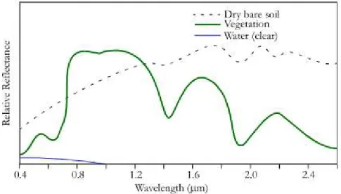
Although the usage of the visual spectrum to generate spectral response pat-terns may be enough in some cases, this is not always the case. For example, figure 2.2 shows a signature for vegetation along water and dry soil. It can be seen that in the visible spectrum (approximately 0.4 to 0.8 µm) the reflected values are different but relatively close, and when the spectrum contains more information, in this case regarding infra-red wavelengths (>0.8 µm), it can be seen that the patterns are even more distinct in this region, facilitating the identification of the different classes. Analyzing and classifying spectral response patterns is the basis of land cover classification.
2.1. SPECTRAL SIGNATURES
Given the importance of bands capturing not only the visible spectrum, but other regions of the electromagnetic spectrum, it is not surprising sensor systems came to include multiple bands capturing this information. For example, Landsat 8 has eleven bands, five of which are dedicated to the infra-red zone of the spectrum, as seen in table 2.1 in page 15.
In addition to multi spectral imagery, some systems such as AVIRIS (Airborne Visible/Infrared Imaging Spectrometer) and MODIS (Moderate Resolution Imag-ing Spectroradiometer) are capable of capturImag-ing hyperspectral data. These systems cover virtually the same wavelengths as the multi spectral ones, but capture data in much narrower bands. This can increase the number of bands and precision avail-able for image classification, as well as the computing power and time necessary for them.
2.2
Sensor/Platform Systems
A variety of platforms are available for the capture of remotely sensed data. Of those, the most important ones when it comes to land cover classification, are aerial photography and satellite-based systems.
2.2.1
Photography
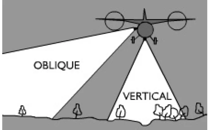
Aerial photography is the oldest and most widely used method of remote sensing. Cameras are mounted in aircraft flying between 200 and 15,000 m and capture a large quantity of information. Aerial photos provide an instant visual representa-tion of the earth’s surface and can be used to create detailed maps. Camera and platform configurations can be grouped as oblique or vertical.
Oblique aerial photography is taken at an angle to the ground. The resulting images give a view similar to an observer looking out of an airplane window. These are easier to interpret than vertical photographs, but difficult to use for mapping purposes.
Figure 2.3: the difference between oblique and vertical photography Source
utexas.edu - Survey Methods
2.2. SENSOR/PLATFORM SYSTEMS
2.2.2
Satellite-Based Systems
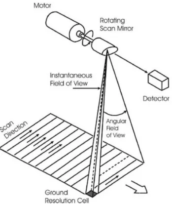
Although aerial photography has proven to have an important part in the field of remote sensing, the development of satellite platforms, the need to transmit imagery in digital form and the desire for highly consistent imagery have given rise to the development of satellite-based scanning systems as a major format for the capture of remotely sensed data (Eastman (2003)).
The basic logic of a scanning sensor is the use of a mechanism to sweep a small field of view - known as an instantaneous field of view (IFOV) in a west to east direction at the same time the satellite is moving in a north to south direction. Together, this movement provides the means to produce a complete raster image of the environment. Figure 2.4 demonstrates how this system works. A rotating mirror captures the energy contained in the IFOV and separates it into its spectral components. Photoelectric detectors then provide the electrical measurements of the amount of energy detected in each of its defined spectrum, for example, one such detector measures the visible red reflectance, another one measures the infra-red one, etc.
Figure 2.4: Simple mechanism of satellite-based systems. Source what-when-how.com - Imaging System Types (Visible Imagery) (Remote Sensing)
Characteristics relevant in each system are the spatial resolution, spectral resolution and temporal resolution. Spatial Resolution refers to the size of the area on the ground summarized by one pixel on the image - for example, most Landsat bands have 30 meters of spatial resolution (i.e. one pixel corresponds to a 30 by 30 meter area). Spectral resolution refers to the number and width of the spectral bands that the satellite sensor uses. Temporal resolution in this context means the rate at which images from the same location are captured with the same observation angle.
There are multiple satellite systems in operation today collecting imagery, each has one or more actual satellites. Examples of these systems are Landsat, which will be the one providing data for this study, theSystème Pour L’Observation de la Terre(SPOT), the Advanced Very High Resolution Radiometer (AVHRR), the Moderate Resolution Imaging Spectroradiometer (MODIS), among others.
2.2.3
Landsat
The Landsat program is the longest running enterprise for acquisition of satellite imagery of Earth. For four decades this program, a joint initiative between the United States Geological Survey (USGS) and the National Aeronautics and Space Administration (NASA), has provided unique resources for those who work in various areas such as agriculture, geology, forestry, regional planning, education, mapping, and global change research. Landsat images are also invaluable for emergency response and disaster relief.
As of this writing there have been eight Landsat satellites, the first of which was launched in 1972, while the most recent one - Landsat 8 - was launched in February 11, 2013. In the context of this work, the satellite providing data will be the Landsat 8.
Landsat 8
The most recent Landsat satellite, Landsat 8 was launched by NASA on February 11, 2013, from the Vanderberg Air Force Base, California. It joins the Landsat 7 on orbit, providing increased coverage of the Earth’s surface. It currently has a planned mission duration of five to ten years.
2.2. SENSOR/PLATFORM SYSTEMS
found on earlier Landsat satellites, providing some degree of compatibility with historical Landsat data. There are two new spectral bands, one for coastal water and aerosol studies (band 1), and a band for cirrus cloud detection (band 9).
The second one is the Thermal InfraRed Sensor (TIRS), built by the NASA Goddard Space Flight Center. It was added to continue thermal imaging and to support emerging applications such as modeling evapotranspiration for monitor-ing water use consumption over irrigated lands. The TIRS collects data in two long wavelength thermal infrared bands and has a 3-year expected life.
Table 2.1: Landsat 8 Sensor Bands.SourceU.S.G.S. (2013)
Sensor Band Spectral range (µm) Pixel Size (m)
OLI
1 - Coastal/Aerosol 0.43 - 0.45 30 x 30
2 - Blue 0.45 - 0.51 30 x 30
3 - Green 0.53 - 0.59 30 x 30
4 - Red 0.64 - 0.67 30 x 30
5 - Near Infrared 0.85 - 0.88 30 x 30 6 - Short-wave Infrared 1 1.57 - 1.65 30 x 30 7 - Short-wave Infrared 2 2.11 - 2.29 30 x 30 8 - Panchromatic 0.50 - 0.68 15 x 15 9 - Cirrus 1.36 - 1.38 30 x 30
TIRS 10 - Thermal Infrared 1 10.60 - 11.19 100 x 100 * 11 - Thermal Infrared 2 11.50 - 12.51 100 x 100 *
*TIRS bands are acquired at 100 meter resolution, but are re-sampled to 30 meter in the delivered data product.
Table 2.1 describes the bands used in the OLI and TIRS Landsat 8 sensors. Like its predecessors, the Landsat 8 has a temporal resolution of 16 days, and the scenes captured have also an area of 170 km by 185 km. However, one noticeable change the Landsat 8 brings is the fact Landsat 8 sensors provide improved signal-to-noise radiometric performance quantized over a 12-bit dynamic range. This translates into 4096 potential grey levels, compared with only 256 grey levels in previous 8-bit instruments. Improved signal to noise performance enables improved characterization of land cover state and condition. The 12-bit data is scaled to 16-bit integers and delivered as such to the public.
(a) Bands 4,3,2 combined (Red, green and blue)
(b) Bands 5,4,3 combined (Infrared, red and green)
Figure 2.5: Example of images obtained by combining various bands
Figure 2.5 shows an example of different information obtained by combining different bands, and how the infrared band in the second image provides infor-mation about the crops around the Tagus river (our region of study) by being distinctively more red in those.
2.3
NDVI
Live green plants absorb solar radiation in the spectral region of about 400 to 700 nanometers, which they use as a source of energy in the process of photosynthesis. This spectral region roughly corresponds with the range of light visible to the naked eye. Plants also scatter solar radiation in the near-infrared region of the electromagnetic spectrum. Thus, green plants appear darker in this 400 to 700 nanometer region, and brigther in the near-infrared. Unlike this, other captured types of data, such as snow, clouds, pavement, dry soil, do not exhibit these properties.
2.4. IMAGE CORRECTION
have medium to high positive values, where other areas will have small positive values, or even negative. The index is defined as follows:
NDV I = (N IR−RED) (N IR+RED)
Since after the image correction, both bands will have values between 0 and 1, the NDVI band will have values between -1 and 1. This index is used instead of other possible ones, such as simply (N IR/RED), which, despite having advantages (such as being always positive), can also have disadvantages, mainly the possibility of having a mathematically infinite range, from 0 to infinity.
Since the NDVI band is used in this field, mainly for visual interpretation of an image, it was interesting to see how relevant it would be in the actual classification process of this work, since it did not really offer any new values by itself, being a result of the above equation, only a new relation between bands.
2.4
Image Correction
There was some image preprocessing applied to all the images used in this work, these are composed of 16-bit unsigned integers with values 0 to 65536 that were converted to top of atmosphere (TOA) reflectance values, which are the actual real values recorded by the satellite - these are more sensible to small changes in land cover which can help the goal of this work. This process was performed by prof. Adélia Sousa, and is the Conversion to TOA reflectance provided by USGS onUSGS - Using the USGS Landsat 8 Product.
2.5
Land Cover Classification Methods
There are two general approaches used to classify land cover into classes, su-pervised and unsusu-pervised classification (Eastman (2003)). They differ on how the classification is actually performed. In supervised classification the software system identifies specific land cover types from the input data, through a series of known examples in the image, known as training data. With unsupervised classification, the system separates the image points into clusters that will be later classified manually.
Supervised Classification
There are three steps to supervised classification. First, a set of training points is selected for each class. This may be done using information collected by a variety of methods such as ground surveys, aerial photography, or any other source of reference data. The system is then used to develop a statistical characterization of the reflectances for each class. Finally, the image is then classified by examining the reflectances of each point and deciding which of the classes it resembles most.
Unsupervised Classification
In contrast to supervised classification, unsupervised classification requires no advance knowledge about the classes of interest. It examines the data and breaks it into the most prevalent spectral groupings, or clusters, present in the data. After this clustering procedure is done, it is then the analyst’s job to identify those classes by associating a sample of pixels in each class with available reference data.
2.5. LAND COVER CLASSIFICATION METHODS
The two previous concepts are not only related to land cover classification, they are fundamental to the area of machine learning as a whole (Han et al. (2006)). However, there are two other concepts more specific to land cover classification: pixel-based classification and object-based classification.
Pixel-based Classification
As the name implies, pixel-based classification is done by trying to classify ev-ery pixel of the original image independently of each other. This approach has some issues such as the fact pixels might contain more than one class, which might contribute to the misestimation of the land being higher than expected (Foody (2002)).
Object-based Classification
A recently new concept in remote sensing, object-based classification has its first step as image segmentation - grouping the pixels in the image into objects.
This approach uses an algorithm that begins with pixel sizes objects which are iteratively grown through pair-wise merging of neighboring objects based on several user-defined parameters (scale, color , shape, smoothness, compactness, etc.) that are weighted together to define a homogeneity criterion; together, these parameters define a "stopping threshold" of within-object homogeneity based on underlying input layers, and thus define the size and shape of resulting image ob-jects (Duro et al. (2012)). After this separation into obob-jects, this approach classifies each object by themselves, instead of each pixel.
A number of studies have been done in these areas, both comparing classifica-tion algorithms themselves and comparing pixel and object-based classificaclassifica-tion methods, they will be discussed in sections 2.5.1 and 2.5.2, respectively.
2.5.1
Algorithm Comparisons for Land Cover Applications
This section presents an overview of the different classification algorithms used for Land Cover applications. A summary is presented in table 2.2. Regarding algorithm comparison, according to the studies there is a lot of variance in the results provided.
Huang et al. (2002) compared four classification algorithms: support vector machines (SVMs), decision trees (DTs), a neural network classifier and the max-imum likelihood classifier (MLC), using pixel-based image analysis of Landsat Thematic Mapper data. Their results suggested a general better performance of the SVM-based classification versus the other three algorithms.
Pal and Mather (2003) compared artificial neural networks (ANNs), DT and MLC approaches using pixel-based analysis for multi and hyperspectral data. They found that DT performs better on multispectral data, but the MLC procedure performs better on hyperspectral data. Gislason et al. (2006) investigated Random Forests (RF) as classification method of a Landsat MultiSpectral Scanner data set. They found that the RF classifier performed better than the DT classifier and was comparable to accuracies obtained by ensemble methods such as bagging and boosting. but considerably faster than these.
Carreiras et al. (2006) used SPOT-4 imagery to assess the extent of agriculture/-pasture and secondary succession forest in the Brazilian Amazon. They used four classification algorithms: quadratic discriminant analysis (QDA), simple classifi-cation trees (SCT), probability-bagging classificlassifi-cation trees (PBCT), and k-nearest neighbors (K-NN). The study showed that PBCT and K-NN performed better than QDA and SCT.
Laliberte et al. (2006) used an object-based approach on Quickbird imagery to compare K-NN with DT. They found that DTs produced better overall classifi-cation accuracies than the K-NN algorithm. Brenning (2009) compared eleven classification algorithms using pixel-based image analysis and Landsat data in automatic rock glacier detection and found that penalized linear discriminant analysis (PLDA) yielded better results than both SVM and RF methods.
2.5. LAND COVER CLASSIFICATION METHODS
2.5.2
Pixel-based Classification versus Object-based
Classification
A mention of studies comparing pixel-based and object-based classification ap-proaches is provided below. These comparisons suggest the latter outperforms the former when comparing classification accuracy.
Oruc et al. (2004) used Landsat 7 imagery to compare pixel and object based approaches in Zonguldak, Turkey. They found object-oriented classification (using a fuzzy classifcation method) produced more accurate results than the pixel-based one.
Whiteside and Ahmad (2005) compared the results of an object-based classification and a pixel-based one for mapping land cover. Their results showed the overall ac-curacy of the object-based classification (using a fuzzy classifcation method) to be marginally better than the pixel-based one. Yan et al. (2006) compared pixel-based classification (with a MLC algorithm) with object-based classification with a k-NN classifier on Advanced Spaceborne Thermal Emission and Reflection Radiometer (ASTER) imagery to identify potential coal fire areas. They found the accuracy of the object-based classification drastically outperformed the pixel-based one by 36.77%.
Platt and Rapoza (2008) compared k-NN and MLC for both pixel-based and object-based classifications with and without expert-object-based knowledge, using IKONOS imagery. Their results found that object-based classification were not better by themselves, but with the addition of expert knowledge had a better overall classi-fication.
Zhou et al. (2008) used quickbird imagery to compare pixel and object-based clas-sification methods for land cover change assessment and found the latter obtained better results than the former.
Cleve et al. (2008) compared pixel and object based classifications using high-resolution aerial photography to plan wildfire mitigation and achieved better results with the object-based classification (using a fuzzy classifcation method). Mohan et al. (2009) used artificial neural networks to compare object-based clas-sification with pixel-based clasclas-sification and found object-based clasclas-sification to have better results.
Castillejo-González et al. (2009) used QuickBird imagery to compare pixel-based and object-based classification in agricultural environments. Five classification methods were used (Parallelepiped, Minimum Distance,Mahalanobis Classifier Distance,Spectral Angle Mapper and MLC) They found both methods achieve
similar accuracy higher than 80%, both using the MLC classifier.
Weih Jr and Riggan Jr (2010) compared SPOT-5 satellite imagery on both object-based and pixel-object-based classification and found the former to have better results. Myint et al. (2011) too used QuickBird imagery to classify urban land cover, and found better results using the object-based classifier using k-NN.
Dingle Robertson and King (2011) compared pixel-based and object-based im-age analysis for classifying agricultural land cover types and assessing change over time periods (1995 and 2005) using Landsat 5 imagery. They found both approaches were very similar regarding accuracy, although object-based classifica-tion had problems such as the absorpclassifica-tion of small rare classes into larger objects. However, a post-classification intensive visual analysis suggested the object-based classification (using k-NN) depicted change more accurately than the pixel-based classification using MLC.
Devadas et al. (2012) found a distinct advantage of object-based methods over pixel-based ones using Landsat 5 and 7 data with SVM classification.
Duro et al. (2012) compared SVM, DT and Random Forest approaches to both classification methods and found object-based ones to be always better than their pixel-based counterparts and SVM to be the better overall approach.
Jebur et al. (2013) compared pixel-based (with DT and SVM approaches) and object-based (SVM) classification and found the object-based approach to be better overall.
2 .5 . L A N D C O V E R C L A S S IF IC A T IO N M E T H O D S
Table 2.2: Article results summary for algorithm comparisons
Article Research Goal Best Classifiers
Huang et al. (2002) General comparison SVM
Pal and Mather (2003) General comparison DT, MLC
Gislason et al. (2006) General comparison RF
Carreiras et al. (2006) Assess extent of agriculture/pasture and forest PBCT, K-NN
Laliberte et al. (2006) General comparison DT
Brenning (2009) Rock glacier detection PLDA
Otukei and Blaschke (2010) Assess land cover changes DT Rodriguez-Galiano et al. (2012) General comparison RF
Oruc et al. (2004) General comparison Fuzzy Classifier Whiteside and Ahmad (2005) General comparison Fuzzy Classifier Yan et al. (2006) Identify potential coal fire areas K-NN
Platt and Rapoza (2008) General comparison K-NN, MLC
Zhou et al. (2008) Assess land-cover changes Rule-based classification Cleve et al. (2008) Wildfire mitigation Fuzzy Classifier Mohan et al. (2009) General comparison Neural Networks Castillejo-González et al. (2009) Crop detection MLC
Weih Jr and Riggan Jr (2010) General comparison Principal Component Analysis
Myint et al. (2011) General comparison K-NN
Dingle Robertson and King (2011) Crop detection, Assess land cover changes K-NN
Devadas et al. (2012) General comparison SVM
Duro et al. (2012) General comparison SVM
Jebur et al. (2013) General comparison SVM
2.5.3
K-Nearest Neighbor
The K-nearest neighbor (K-NN) method is one of the most fundamental and simple classification methods, it was introduced by Fix and Hodges Jr (1951). It is a very simple algorithm where every point is classified based on the pre-specifiedkvalue, the number of closest training samples in the feature space by a majority vote. For example, if k =1, the object is simply assigned the class of its nearest neighbor. To prevent ties regarding voting, an odd value ofkis usually chosen. Different distance metrics exist, such as Euclidean distance, Manhattan distance, Hamming distance, among others, depending on its usefulness for specific problems. The Euclidean distance is the most common approach on general problems. A simple algorithm description is as follows:
For each point p, having a known set Lof data points, the distance betweenp and every point of Lis calculated. The distances are sorted in increasing numerical order and the firstkelements are picked. Finally a majority vote is done to decide the classification of p.
Figure 2.6 shows an example of a simple 2-Dimensional K-NN classification and the relevance ofkvalues, the green point should be classified in either red triangle or blue square classes. If k = 3 it’s assigned to the red triangle class (solid line circle), ifk=5 (dashed line circle) it’s assigned to the blue square class.
2.5. LAND COVER CLASSIFICATION METHODS
2.5.4
Decision Trees
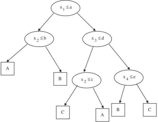
Decision tree classification (Quinlan (1986)) is a common method used for classi-fication. Unlike other methods that use all available features at once by making a single complex decision, decision trees work by partitioning the problem into smaller subproblems and defining a set of rules to be followed sequentially down a tree-like structure (Pal and Mather (2003)).
The algorithm works by initially constructing the actual tree, by splitting the training data into subsets based on tests on the features in a process called recursive partitioning. This process is then repeated on each derived subset. This recursion is stopped once splitting subsets no longer adds value to the predictions. Labels are then assigned to the terminal (leaf) nodes.
Figure 2.7: decision tree exampleSourcePal and Mather (2003)
For the actual classification, the tree structure is simply followed sequentially from the root until a leaf node is reached by analyzing the test data features. Figure 2.7 shows a simple example of a classification tree. Thexiare the feature values, A,BandCare the class values. Assuming we follow the left child if the tests are positive and right nodes if not, a point where x1 ≤aand x2 >bwill be classified as the classB.
A number of parameters can be relevant to the tree construction, with the most relevant (Atkinson and Therneau (2000)) beingminsplitandcpin R (Section 2.7).minsplitis the number of minimum observations that must exist in a node for which a split will be attempted.cpis the cost complexity factor, for example, a value of 0.001 defines that a split must decrease the overall lack of fit by a factor of 0.001 before being attempted. Of these, this study will use onlycp, since it is the only one available through the caret package (Subsection 2.7.1).
2.5.5
Random Forests
The basis of Random Forests are Decision Trees, these are mentioned in the pre-vious subsection. Decision trees can be used multiple times, such as in bagging or boosting. In boosting, successive trees give extra weight to points predicted incorrectly by earlier trees. In the end, there is a weighted vote taken for prediction. In bagging, each tree is independently constructed using a bootstrap sample of the data set, then a majority vote is taking for prediction. Liaw and Wiener (2002)
An additional layer of randomness is added by random forests, proposed by Breiman (2001). In a random forest model, during training, a number of decision trees are created, each having as basis a different training data subset by resampling randomly the original training dataset with replacement. Along with this random subset of the training data, the features each tree receives are themselves a random subset of the original features. This allows for greater classifier stability and increases classification accuracy (Breiman (2001)).
2.5. LAND COVER CLASSIFICATION METHODS
2.5.6
Support Vector Machines
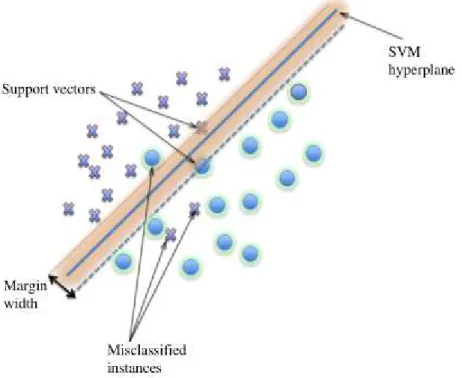
Support vector machines (SVMs) is a supervised learning technique used in classi-fication introduced by Cortes and Vapnik (1995). In its simplest form, SVMs are linear binary classifiers that assign a given test sample a class from one of two possible labels by separating the data through a hyperplane (line in 2 dimensions, plane in 3 dimensions, etc). An instance of the data to be labeled in the case of remote sensing is for example, an individual pixel. Figure 2.8 identifies an example of this scenario in 2 dimensions.
Figure 2.8: simple support vector machine example. Source Mountrakis et al. (2011)
However, there are situations where the data isn’t separable in the current dimensions. Figure 2.9 exemplifies this, on the left, in 1-D the blue and orange points cannot be separated, however, by applying the transformationx→ (x,x2), we get the data set shown on the right, from which a hyperplane can be found that separates the data correctly. One such example is the line shown in red. This is called a kernel - a transformation of the input data that allows algorithms such as SVMs to process it more easily. There are a number of existing kernel functions. In this work the one used will be the (Gaussian) radial basis function kernel.
Figure 2.9: a harder caseSourcequora.com - What are Kernels in Machine Learning and SVM?
SVMs have proven a very reliable method in processing of remote sensing data (Mountrakis et al. (2011)). Since remote sensing will almost always deal with mul-tiple classes and not two, adjustments are made for the SVM algorithm to operate as a multi-class classifier. The dominant approaches for this are constructing a number of binary classifiers, such as the one-vs-all approach, where the classifier with the highest output function assigns the class, and the one-vs-one approach, where every pair of classes is tested against each other, and classification is done by a voting strategy.
The parameters for this Gaussian kernel in particular are C - Cost andγ- gamma, C controls the cost of misclassification on the training data. The gamma parameter defines the influence of a single training point, with low values meaning high influence, and high values meaning low influence.
2.5.7
Maximum Likelihood
The maximum likelihood classification method is a very simple and common method, ubiquitous in every geographic information systems software, such as ESRI’s ArcGIS suite (Esri) and Exelis’ ENVI suite (Exelis Visual Information Solu-tions). This method is described more extensively by Richards and Richards (1999).
2.6. EVALUATION MEASURES FOR DATA CLASSIFICATION
2.6
Evaluation Measures for Data Classification
2.6.1
Cross-validation
Cross-validation is a model validation technique for assessing how the results of a model will perform in a new data set. In a prediction problem, a model is given a dataset of known data in which to train (training dataset), and a dataset of data against which the model is tested (testing dataset). The model "learns" with the training dataset, and then receives the testing dataset, outputting the predictions, which are then compared with the real classes of this dataset, yielding results such as accuracy.
The goal of cross-validation is to define a "test" dataset to test the model in the training phase, in order to try to limit issues such as overfitting, and give an insight on how the model will probably perform in the real testing dataset, and, if the model has parameters, cross-validation also allows for these to be tuned, so the best ones can be used in the testing phase. For example, in this work, cross-validation is performed for k-NN (and others), where different values of k are tested using cross-validation and the best of these is chosen as the "true"kvalue to use for the actual testing phase. Thesek’s do not mean the same thing, in k-NN, k means the number of neighbors and regarding cross-validation, it means the number of folds to split data in.
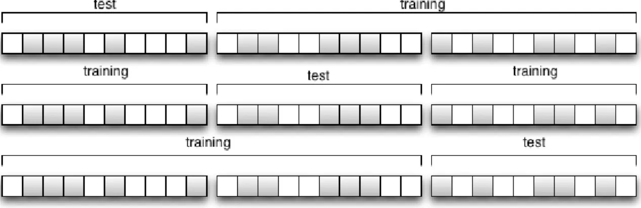
Figure 2.10: Example of 3-fold cross validation.Sourcein.ed.ac.uk - Dispel Tutorial 0.8 documentation - k-fold cross validation
There are many different ways to partition the training dataset to perform this analysis. In this work, 3-fold (k=3) cross validation will be used. In k-fold cross validation, the original training data is split intokequal subsample sets, where one is retained as the validation data for testing, andk−1 used as training data. This is repeatedktimes, with each of the subsamples being used exactly once as validation data. Thekresults from this analysis can then be averaged to produce a single estimation. Figure 2.10 shows an example of 3-fold cross validation in a dataset containing originally 30 training samples.
2.6.2
Confusion Matrix
A confusion matrix is a specific table layout that allows for visualization of an algorithm’s performance, by comparing the results of the predicted classes with the true class labels - each column represents the instances of a predicted class while rows represent the instances in an actual class, or vice-versa. This work uses the former whenever a confusion matrix is available. The name confusion matrix stems from the fact these tables allow for easy interpretation of whether two classes are being misclassified as one another (confusing the classes).
Table 2.3: simple three-class confusion matrix
Cats Dogs Rabbits Total
Cats 5 3 0 8
Dogs 2 3 1 6
Rabbits 0 2 11 13
Total 7 8 12 27
Table 2.3 shows an example of a confusion matrix for a system trying to classify animals into cats, dogs or rabbits, there are 27 samples, 8 cats, 6 dogs and 13 rabbits. It can be seen that from the 8 actual cats, the system predicted 5 correctly and 3 to be dogs, for example, also it predicted one dog to be a rabbit, among other predictions. All correct guesses are located in the diagonal of a table making it easy to inspect the table for errors, which are the values outside of the diagonal.
2.6. EVALUATION MEASURES FOR DATA CLASSIFICATION
2.6.3
Cohen’s Kappa coefficient
Cohen’s Kappa coefficient (Cohen (1960)) is a statistical measure of inter-rater agreement for qualitative (categorical) items. It is generally thought to be more robust than simple percent agreement calculation, since it takes into account the agreement occurring by chance. The equation for kappa is
k= (po−pe) (1−pe)
where pois the relative observed agreement andpethe hypothetical probability of chance agreement. If the raters are in complete agreement thenk = 1, while if there is no agreement among the raters other than what would be expected by chance,k <0. A simple two class example follows, with a confusion matrix in a example system trying to classify cats and dogs.
Table 2.4: simple two-class confusion matrix
Cats Dogs Total
Cats 10 5 15
Dogs 7 8 15
Total 17 13 30
From the confusion matrix, we can see there is a total of 30 classified instances, where 15 (10 + 5) were cats, 15 were dogs (7+8), and there were 17 instances classified as cats, and 13 as dogs. po in this case is simply the total number of correctly classified instances in the entire matrix, divided by the total number of instances, as such: 0.6((10+8)/30).
To calculate pe, we first multiply the marginal frequency of cats for one "rater", by the marginal frequency of cats for the second "rater", and divide by the total number of instances. The marginal frequency for a certain class by a certain "rater" is just the sum of all instances the "rater" indicated were that class. In this case, we have 15 cats and 17 classified cats, resulting in a value of 8.5((15∗17)/30), this is also done for the second class, yielding a result of 6.5((15∗13)/30). The final step is to add these values together and divide them by the total number of instances, yielding a pe value of 0.5((8.5+6.5)/30).
Kappa is then calculated, yielding a value of 0.2,(0.60−0.50)/(1−0.50). This measure was included since it was, along with simple accuracy, used in the great majority of studies in table 2.2.
2.7
Used Technologies
We will make use of R, a multi-platform open-source language and software for statistical computing (R Core Team (2013)). It is a highly used tool in this field and has several add-on packages that will be helpful in this work. Esri’s ArcGIS suite (Esri) will also be central to this work.
2.7.1
R Packages
The main packages used in this work were:rgdal,caret,raster,randomForest,rpart, kernlab
Additional packages not mentioned might have been used, possibly as depen-dencies of these mentioned, in any way, a comprehensive list of all the packages installed in the system is provided for clarity, and is available in appendix A.
Caret
2.7. USED TECHNOLOGIES
2.7.2
Shapefiles
The shapefile format is a highly popular geospatial vector data format used in geographic information system software. This format was developed and is main-tained by ESRI, as a specification for data interoperability between ESRI and other GIS products (Esri). This format can describe points, lines and polygons, to represent any kind of information wanted as items.
Figure 2.11: Example of information represented by shapefiles.Sourcewikipedia.org - Shapefile
Figure 2.11 shows an example of information represented by a shapefile. In it, it can be seen that points represent wells, lines represent rivers and a polygon represents a lake. Each item usually has attributes that have some information about it, such as name or temperature. The shapefile format does not consist of only one file, but a set of files, some optional and some mandatory that have a common prefix, stored in the same directory.
This is a fundamental format used for this work, it is the format in which information is saved, to be used by the R scripts (for this work, polygons were used, where all the points inside were defined as one of the classes used). From it, and the image layers, the necessary data for this work is obtained, by extracting, for each point inside of the polygon the correspondent values in each of the image layers.
2.8
Summary
It can be seen that remote sensing is a large field where a number of studies have been done. Regarding classifiers, the best results for land cover classification usually arise from Support Vector Machines, Decision Trees, Random Forests, Max-imum Likelihood Classifiers and the K-Nearest Neighbor algorithm, as can be seen in table 2.2, both when using pixel-based and object-based approaches. Regarding the comparison between these approaches, it can be seen that generally the classi-fication results are better when using the object-based classiclassi-fication. However, the pixel-based approaches still manage to obtain high accuracy percentages. For this work, those classification methods were chosen, and a pixel-based approach was used, since object-based ones introduce unnecessary layers of complexity to this work.
C
H
A
P
T
E
R
3
S
YSTEM DEVELOPMENT
In this chapter, the development of the created system will be described. Ini-tially, information will be provided about the environment where the study was conducted, as well as how the results can be reproduced. After that, the data preparation performed, where raw data is transformed into acceptable input to the study, will be extensively described. Finally, the work performed in R will also be described, the main work phases separated into single and multiple image parts.
3.1
Preliminary Work
As of this document’s writing, the preliminary work done on this work was a ground survey made on July 2013 by Prof. Adélia Sousa and Prof. José Rafael Silva, that assigned a classification to some points of the study area. These points are the fundamental basis of our work since they would then be used as training/testing data.
3.2
Approach
1. Landsat 8 imagery of our study area from July 2013 (the same month as the previously done ground survey) was acquired from online archives. A crop of the original images was done, since they are much larger than necessary for this study and it would considerably slow the following steps.
2. About nine thousand points of ground truth data were obtained based on a previously done ground survey around that time, that assigned a classifi-cation to some points in the area. The bands used are bands 2-7 according to table 2.1, capturing the visible and infrared zones of the electromagnetic spectrum, since those are the best bands to use for land cover classification (USGS - What are the best spectral bands to use for my study?).
3. The main crop classes used were:
• Potato
• Vineyard
• Rice
• Tomato
• Maize
Other classes were also be used to facilitate the distinction between land cover types, described in Subsection 3.4.1.
4. The classification was done using the R as mentioned in Subsection 2.7, since it is a notorious tool in this field that provided us with implementations of the classification methods chosen. In R, several packages were used to classify the image data, five classification algorithms were used:
• Support Vector Machines
• Random Forests
• Maximum Likelihood Classifier
• K-Nearest Neighbor
• Decision Tree
3.3. SYSTEM INFORMATION/RESULTS REPLICATION
3.3
System Information/Results Replication
The largest portion of this work was done using the R language, since, as men-tioned in Section 2.7, it is a very appropriate language to perform this kind of analysis on, it is widely used in this field, and it contains a number of useful packages (e.g. loading the data from the shapefile, classification algorithms). In this section the packages and folder structure used will be explained, along with a brief description of each file and its function. The version used was R version 3.1.2 (2014-10-31) under Windows 7 x64, RStudio version 0.98.1102 was used as an IDE since it provides a helpful interface compared to running R in a simple command line interface.
3.3.1
Folder structure
A simple folder structure is as follows: thesis
inputs
shapefiles
<all layer folders>
mlc
outputs
The thesis folder is the main folder, containing the inputs, mlc and outputs folders. It has the main R scripts, themlc folder has the Maximum Likelihood Classifier implementation, theinputsfolder contains theshapefilesand the image layers’ folders for each date. The shapefiles folder contains the shapefiles, and the each layer folder contains the seven layers (blue, green, red, near-infrared, short-wave infrared 1, short-wave infrared 2 and NDVI) for that date. Theoutputs folder contains the generated images. These were mostly created for the sake of organization, and as such, there is no issue in editing the R scripts to load files from different locations, if necessary.
A brief description of the R scripts contained in the main folder follows, for more information, all the scripts are highly commented and available in the appendix.
loader.R
Loads the shapefile and image layer values, extracts the values of the points inside the shapefiles for those images, and joins them in a data frame ready to be used by the rest of the scripts.
plotHistogramas.R
Plots the imagery seen in Subsection 4.2.1 into box-plots.
si_decisionTree.R
The decision tree algorithm is applied, before this, loader.R is ran, data is split into training and test data, then split for cross-validation, then the grid is set up. After, results are collected and the full image is generated.
si_kNN.R, si_MLC.R, si_randomForest.R, si_SVM.R Same as above for the other algorithms.
percentages.R
Yields the results of Subsection 4.2.3.1 - the study on how important is using 100% of the data versus 25,50 and 75%.
multi_loader.R
Same as loader.R, to be ran in the following scripts, loads the new image data for testing (so all the data from loader.R is for the training set).
multi_randomForest.R
Runs loader.R, sets the data as training set, trains it, runs multi_loader.R, sets the new data as test set, collects results and generates the new image.
multi_SVM.R
Same as above, for SVM.
mlc.R
3.4. DATA PREPARATION
Maximum likelihood classifier adaptation
Unlike the four other methods, the Maximum Likelihood Classification algorithm was not available on thecaretpackage, this would not be a problem in itself since this method has no parameters to actually perform tuning on (which was the main reason for using thecaretpackage), but there were no other implementations of this method found that would work with the same data format as used by our scripts.
The rasclasspackage contained one method that supported a different input format - however, changing the data to this format just to use it on this classification algorithm was deemed an unnecessary step, more convoluted than simply trying to modify the existing algorithm to fit our needs, and, as such, its maximum likelihood classification function was extracted and adapted to be used with our data formats, therasclasspackage licenses are the GNU General Public License version 2 and 3 so there is absolutely no issue regarding modification of the code.
3.3.2
Result replication
TheplotHistogramas,si_*andpercentagesscripts can all be ran independently. This was intended and the reason there is some similar code in these. There are no changes necessary to be made to reproduce the Section 4.2.1, Section 4.2.2 and 4.2.3.1 results, simply running the scripts is enough. To reproduce the results from the other complementary studies (sections 4.2.3.2 and 4.2.3.3, the loader.R file is modified to receive the original bands with no image correction in the former, and to ignore the last band (NDVI) in the latter, and then thesi_*scripts can be ran.
For the multi-image phase, it’s merely a matter of modifying theloader.Rand multi_loader.Rto set up what image dates are wanted from the available ones, and then running themulti_*files.
3.4
Data Preparation
There is a need for some data preparation before the actual classification is done in R. This work can be divided into two parts, regarding the shapefile and the image layers used.
3.4.1
Shapefile Preparation
Regarding the shapefile, the original shapefile was compiled by Prof. Adélia Sousa as mentioned in Section 3.1, it was the result of ground visits within days of the satellite images were acquired, to obtain the best accuracy possible. This shapefile, however, needed some modifications because it contained samples from classes not relevant to this work (i.e. not the five main classes from 3.2), mostly because their sample size was too low both in the collected data and in the study region.
These classes were deleted from the original shapefile. This was the first step regarding the shapefile modification. All the shapefile modifications mentioned in the following paragraphs were done in ArcGIS’ training sample manager - this creates a specific shapefile format that the R scripts process (for example, the R scripts assume the class name column is called Classnamein the shapefile, and the spectral values are present on columns numbered 7 to 12, or 13 with NDVI), however, if necessary, the R scripts can be very easily edited to adapt to other custom shapefile formats. When classes were added it means there were a number of polygons created that contained enough points to be useful in classification, these were then merged and classified as one class.
3.4. DATA PREPARATION
This modified shapefile was used during some time for the classification (with roughly the same results as the final one), but ultimately it was necessary to make some changes for a better visual interpretation of the image, discovered after the generation of the classified images in R. There were two main issues:
Misclassification of large parts of vegetation near the image boundaries
Large parts of vegetation that had no specific class assigned were being classified as "Vineyard", this had no impact on the classification accuracies in itself, and as such was not an issue that could be detected during the result analysis of the classification algorithms. It was only after visual interpretation of the image that this became noticed as an issue. To fix this issue another class was created to classify this extra vegetation, that fixed most of these visual issues.
Misclassification of small roads between crops
Small roads between crops were also being misclassified, another issue only uncovered after visual interpretation of the results. Again, this did not impact the classification accuracy, but for the sake of visual interpretation it was a problem that could be addressed. These were also mostly being misclassified as "Vineyard". This was a harder problem to solve, mainly because adding training samples of these small roads was very hard, since the image pixels corresponded to 30x30m areas, these roads were barely visible in some areas. Some small polygons were created and temporarily made an extra "Small Roads" class, but eventually it was merged with the "Other" class since it provided roughly the same information.
The final shapefile contained, then, information about nine classes, the "main" five - Maize, Vineyard, Rice, Tomato, Potato, and four extra classes - Stover, Vege-tation, River and Other.
3.4.2
Layers Preparation
The first step in processing the layers was to apply image correction to each layer. This was done by Prof. Adélia Sousa.
After that, an important step was to delete most of the image, the original image obtained from USGS was too big and most of it was of no relevance to this work, compared to the area of which we have training samples. Classifying the whole image would, then, be an unnecessary process that could be avoided, because it would provide no relevant information, and mainly because it would dramatically increase the generation time of the final images.
A rectangle-shaped crop was applied to all the image layers, making sure it covered all the training sample polygons but not much more than that. This was done in ArcGIS by creating a rectangle-shaped shapefile, and then using the Spatial Analyst Toolbox - Extract by Mask option, with each layer and this rectangle shapefile as inputs, receiving the cropped layer as output.
Finally, the NDVI (Section 2.3) band was generated, this was also performed in ArcGIS using its Raster Calculator option. Since this band was "artificially" generated there was some curiosity regarding its impact in the classification procedure, a simple study of the relevance of the NDVI band was performed.
C
H
A
P
T
E
R
4
E
XPERIMENTAL
S
TUDY
In this chapter, the work phases performed are described, and the obtained results for these are presented, along with discussion of these results.
4.1
Work Phases
4.1.1
Single-image phase
4.1.1.1 Pre-Classification
Before the classification was actually done, a simple script was created to plot the box-plots for each different class, for each band (filew0_plotHistograms.R). This was not a part of the actual classification procedure, but instead, provides a first look at how different the spectral signatures for the different classes were, and a way to visually extract some preliminary information from these. The results of this script are nine box-plots (or, if applied to other shapefiles,Nbox-plots, N being the number of different classes).
4.1.1.2 Classification
In the first main part of this work, the five classification algorithms were applied to our data. This data contains about nine thousand samples, a very large number compared to most works in the related work (table 2.2). This was achieved by creating five scripts, one for each algorithm. The main steps that describe the action taken by these scripts follows:
Load Data
Theloader.Rfile is executed. This file loads a shapefile, a number of layers, and for each point of the shapefile the correspondent layer values are extracted and put into an entry with the point’s class.
Split Data
The data is split into training and test sets, 66% for the training set, 34% for the test set. This is done with stratified sampling (i.e. the proportion of each class’ samples in the original data is maintained for both these sets).
Split Data (2)
The data is split once more to create three folds for cross validation during the training phase.
Create Grid
The values of the parameters to be tuned are defined, this is called creating a grid by thecaretpackage. For example, for the k-NN algorithm, k is defined as the sequence from 3 to 21 with an interval of 2.
Train/Tuning
The algorithm is ran for each possible grid combination while performing 3-fold cross-validation. The best result is then chosen to be used for the test set. For MLC the whole training data is simply fed to the algorithm.
Test
The test set is fed to the algorithm and predicted classes are received. Those are compared to the actual classes and results such as accuracy/Kappa and confusion matrices are obtained.
Predict Image
The whole image is fed to the algorithm and predicted classes are received, those create then a new image with each pixel having a value from 1 to 9 (or the number of different classes in the shapefile), although it’s obviously not guaranteed it will have all of them, some classes might not be predicted at all, in some extreme cases.
4.1.1.3 Complementary studies
influ-4.1. WORK PHASES
Reduction of the initial data
Since a high number of data points was available, it was interesting to study how the algorithms performed with percentages of this original data. This was done by using 5, 10, 25, 50, 75 and 100% of the original data and comparing the results.
Classification without image correction applied
The importance of the image correction process was also something to study, this was performed by loading the original image layers, instead of those where image correction was performed.
Not utilizing the NDVI band
It was also interesting to study how much the NDVI band contributed to the results, this was simply done by ignoring the NDVI band layer on the loader.Rfile
4.1.2
Multi-image phase
After applying the classification methods to the same image from which the data was extracted, they were applied to a multitude of different images, about two and four weeks around the original image’s date, to analyze how these methods were performing over time. The classifiers were trained using the ground truth data used in the single-image phase, and then the new image was fed to the program to be classified. The accuracy results were then calculated by classifying the same data points existing in the ground truth and comparing the classes of those points with the classified values. After that, the complete image was generated. For this section, only RF and SVM algorithms were used since they were ones where better results were had in the previous section.
This section does not separate the same date’s data into training/test sets, the training set is the original images’ values, and the test set is the new images’ ones, about nine thousand values each, around three times more than the number of test values used in the single-image phase. Since this process used the same ground truth data as in the initial phase, the results are expected to be "worse" -for example, a point that was Maize on the original image and its crops would be collected before the next image was taken, could be "correctly" classified as Stover but in fact it would be marked incorrectly since the original data had the Maize class on that point. The further the image dates are from the original image’s date, the worse their classification accuracies are expected to be.